Universidade Federal de Minas Gerais
Escola de Engenharia
Programa de P´
os-Gradua¸c˜
ao em Engenharia El´
etrica
THE NN-DM METHOD - AN ARTIFICIAL NEURAL NETWORK MODEL FOR DECISION-MAKER’S PREFERENCES
Luciana Rocha Pedro
Tese de Doutorado submetida `a Banca Examinadora designada pelo Colegiado do Programa de P´os-Gradua¸c˜ao em Engenharia El´etrica da Escola de Engenharia da Universidade Federal de Minas Gerais como requisito para obten¸c˜ao do T´ıtulo de Doutor em Engenharia El´etrica.
Orientador: Ricardo Hiroshi Caldeira Takahashi
Belo Horizonte - MG
P372n Pedro, Luciana Rocha.
The NN-DM method [manuscrito]: an artificial neural network model for decision-maker’s preferences / Luciana Rocha Pedro. - 2013.
xviii, 164 f., enc.: il.
Orientador: Ricardo Hiroshi Caldeira Takahashi.
Tese (doutorado) Universidade Federal de Minas Gerais, Escola de Engenharia.
Anexos: f. 145-162.
Bibliografia: f. 136-144.
1. Engenharia elétrica - Teses. 2. Algoritmos genéticos - Teses. 3. Processo decisório por critério múltiplo - Teses. I. Takahashi, Ricardo Hiroshi Caldeira. II. Universidade Federal de Minas Gerais. Escola de Engenharia. III. Título.
“Your act was unwise,” I exclaimed “as you see by the outcome.” He solemnly eyed me. “When choosing the course of my action,” said he, “I had not the outcome to guide me.”
Acknowledgements
To my faithful companion, Paloquinho, for his support at all times.
To my advisor, Ricardo Takahashi, for freedom of thought and his un-conditional support.
To my family that, even distant, always cheer for me.
To the doctors Alexandre Celestino and Rodrigo Cardoso and to my fri-ends Cristine Almeida, Camila Albino, Fernanda Alvarenga, and Adriano Silva for the friendship over the past decades.
To Chrystian, Fernando, and Leonardo for the support in those final mo-ments.
To all my friends for the moments of relaxation and fun.
Abstract
This work presents a methodology based on the multi-attribute utility the-ory to approximate the decision-maker’s utility function: the Neural Network Decision-Maker method (NN-DM method). The preference information ex-tracted from the Decision-Maker (DM) involves ordinal description only and is structured by a partial ranking procedure. An artificial neural network is then constructed to approximate the partial ranking reproducing the DM’s preferences in a specific domain. The NN-DM method is suitable in situa-tions in which a recurrent decision process must be performed considering different sets of alternatives and the same DM.
A hybridization between the NN-DM method and the Interactive Ter-ritory Defining Evolutionary Algorithm (iTDEA) is also developed in this work. Considering the same amount of preference information, the NN-DM method is able to construct a model for the DM’s preferences to guide iT-DEA. Henceforth, no further queries are required from the DM related to similar decision-making problems.
Additionally, an Interactive Non-dominated Sorting algorithm with Pre-ference Model (INSPM) based on NSGA-II is proposed. A slight modification in the diversity maintenance strategy inside NSGA-II enables INSPM to dis-tinguish preferable regions within an estimate of the Pareto-optimal front. A parameter allows the control of the preferable regions density and provides from fronts in which there is no interference from the DM until fronts in which the preferred solution is apparent. In all situations the Pareto-front extent is guaranteed.
Finally, the NN-DM method is adapted to find a model for the DM’s preferences in a polymer extrusion process. The DM’s requirement is filling a matrix expressing the preferences considering ordinal comparisons. The NN-DM method is able to provide a model which sorts the alternatives from the best to the worst one according to the DM’s preferences in a real scenario.
Resumo
Este trabalho apresenta uma metodologia baseada na teoria da utilidade multi-atributo para aproximar a fun¸c˜ao de utilidade de um tomador de de-cis˜ao: o m´etodo NN-DM. A informa¸c˜ao de preferˆencia extra´ıda do tomador de decis˜ao (DM) envolve apenas descri¸c˜ao ordinal e ´e estruturada por um procedimento de ordena¸c˜ao parcial. Uma rede neural artificial ´e ent˜ao cons-tru´ıda para aproximar a ordena¸c˜ao parcial reproduzindo as preferˆencias do DM em um dom´ınio espec´ıfico. O m´etodo NN-DM ´e apropriado em situa¸c˜oes em que um processo de decis˜ao recorrente deve ser realizado considerando diferentes conjuntos de alternativas e um mesmo DM.
Uma hibridiza¸c˜ao entre os m´etodos NN-DM e iTDEA tamb´em ´e desen-volvida neste trabalho. Considerando-se a mesma quantidade de informa¸c˜ao de preferˆencia, o m´etodo NN-DM ´e capaz de construir um modelo para as preferˆencias do DM para guiar o iTDEA. Deste ponto em diante n˜ao s˜ao mais necess´arias perguntas ao DM relacionadas a tomadas de decis˜ao semelhantes. Adicionalmente, o algoritmo INSPM, inspirado no NSGA-II, ´e proposto. Uma ligeira modifica¸c˜ao na estrat´egia de manuten¸c˜ao da diversidade do NSGA-II possibilita ao INSPM distinguir regi˜oes prefer´ıveis em uma esti-mativa da fronteira Pareto-´otimo. Um parˆametro permite o controle da densidade nas regi˜oes prefer´ıveis e fornece desde fronteiras em que n˜ao h´a nenhuma interferˆencia do DM at´e fronteiras em que a solu¸c˜ao preferida ´e aparente. Em todas as situa¸c˜oes a extens˜ao da fronteira Pareto ´e garantida. Finalmente, o m´etodo de NN-DM ´e adaptado para encontrar um modelo para as preferˆencias do DM em um processo de extrus˜ao de pol´ımeros. O requisito ao DM ´e preencher uma matriz que expressa suas preferˆencias con-siderando compara¸c˜oes ordinais. O m´etodo NN-DM ´e capaz de fornecer um modelo que classifica as alternativas da melhor para a pior de acordo com as preferˆencias do DM em um cen´ario real.
Contents
Acknowledgements iv
Abstract v
Resumo vi
Table of Contents x
List of Figures xii
List of Tables xiv
List of Symbols xv
List of Abbreviations xvii
1 Introduction 1
1.1 Organization . . . 6
2 Decision Models 10 2.1 Introduction . . . 10
2.2 Classical Decision-making Methods . . . 11
2.2.1 Introduction . . . 11
2.2.2 ELECTRE Methods . . . 11
2.2.3 AHP Methods . . . 12
2.2.4 ROR Methods . . . 13
2.3 Modeling the DM’s Preferences . . . 15
2.3.1 Introduction . . . 15
2.3.2 Artificial Neural Networks . . . 15
2.3.3 Other Techniques . . . 19
3 Notation and Problem Statement 23
3.1 Multi-Criteria Decision-Making Analysis . . . 23
3.2 Multi-Objective Optimization . . . 26
3.3 INSPM. . . 30
4 The NN-DM Method 32 4.1 Introduction . . . 32
4.2 The NN-DM Methodology . . . 33
4.2.1 Step 1: Domain Establishment. . . 34
4.2.2 Step 2: Ranking Construction . . . 37
4.2.3 Step 3: Artificial Neural Network Approximation . . . 39
4.2.4 Step 4: Performance Assessment . . . 46
4.2.5 DM calls . . . 48
4.3 The Algorithm . . . 49
4.4 Illustrative Examples . . . 50
4.5 Discussion . . . 52
5 The Improved NN-DM Method 55 5.1 Introduction . . . 55
5.2 Step 1 - Domain Establishment . . . 56
5.3 Step 2 - Ranking Construction . . . 57
5.3.1 Dominance . . . 57
5.3.2 The Improved Partial Ranking. . . 58
5.4 DM Calls . . . 59
5.5 The Algorithm . . . 60
5.6 Illustrative Examples . . . 61
5.6.1 Example A . . . 61
5.6.2 Example B . . . 64
5.7 Discussion . . . 67
6 The NN-DM Method And iTDEA 69 6.1 Introduction . . . 69
6.1.1 Interactive Algorithms . . . 69
6.2 TDEA, prTDEA, and iTDEA . . . 73
6.3 Computational Experiments . . . 77
6.4 Discussion . . . 82
7 The NN-DM Method And NSGA-II 84 7.1 Introduction . . . 84
7.2 The Adapted NN-DM Methodology . . . 86
7.2.2 Step 2 - Ranking Construction . . . 87
7.2.3 Step 4 - Performance Assessment . . . 91
7.3 NN-DM Method and NSGA-II . . . 91
7.3.1 Dynamic Crowding Distance . . . 92
7.3.2 Neural Network Dynamic Crowding Distance . . . 93
7.4 The Algorithm . . . 94
7.4.1 NN-DM Model . . . 95
7.4.2 INSPM Main Program . . . 97
7.5 Computational Experiments . . . 100
7.5.1 INSPM and Utility Function . . . 102
7.5.2 INSPM and NN-DM Method . . . 104
7.5.3 Comparison with iTDEA . . . 106
7.6 Discussion . . . 109
8 Polymer Extrusion Process 112 8.1 Introduction . . . 112
8.2 Available Data . . . 113
8.3 Interaction with the DM . . . 115
8.4 The Adapted NN-DM Methodology . . . 119
8.4.1 Step 1: Domain Establishment. . . 119
8.4.2 Step 2: Ranking Construction . . . 120
8.4.3 Step 4: Performance Assessment . . . 120
8.4.4 Algorithm . . . 121
8.5 Computational Experiments . . . 122
8.6 Case Study . . . 124
8.7 Discussion . . . 130
9 Conclusions and Ideas for Future Work 132 Bibliography 136 A The NEWRB Function 145 A.1 Definition . . . 145
A.2 Description . . . 145
A.3 Algorithm . . . 146
A.4 Simulating the Network . . . 147
B A Comparison Between Mergesort and Quicksort 149 B.1 Algorithms. . . 150
B.1.1 Quicksort . . . 150
B.2 Results . . . 152
C Decision-making Matrices - Polymer Extrusion Process 155
List of Figures
1.1 Similar Pareto-optimal fronts. . . 5
4.1 Refinement of a regular two-dimensional domain D. . . 35
4.2 Refinement of a regular three-dimensional domain D. . . 36
4.3 Refinement of a generic domain. . . 36
4.4 Refinement of a Pareto-optimal front. . . 37
4.5 RBF network architecture. . . 40
4.6 Gaussian functions with σ = 1,2,3. . . 41
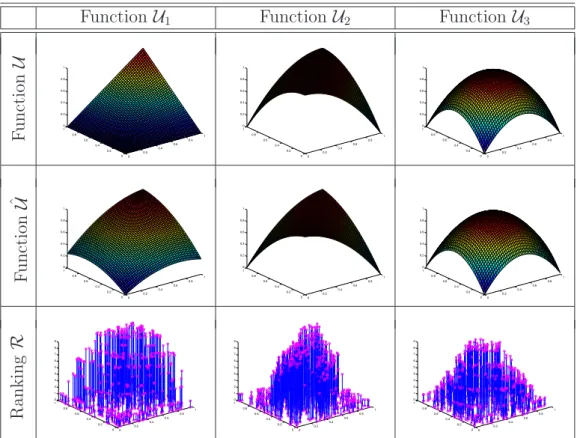
4.7 Surface and level sets of the functionsU and ˆU. . . 45
4.8 Example of a function ˆU being employed. . . 45
4.9 DM’s underlying utility functions. . . 51
4.10 Partial ranking. . . 51
4.11 Models ˆU obtained by the NN-DM method. . . 52
4.12 Partial ranking examples. . . 53
5.1 Domain establishment. . . 57
5.2 DM’s underlying utility function U. . . 62
5.3 Partial ranking with n = 50 alternatives. . . 63
5.4 Model ˆU for the DM’s preferences. . . 63
5.5 DM’s underlying utility function U. . . 65
5.6 Partial ranking with n = 50 alternatives. . . 65
5.7 Model ˆU for the DM’s preferences. . . 66
5.8 Two-dimensional instance: number of queries and KTD. . . . 66
5.9 Three-dimensional instance: number of queries and KTD. . . . 67
5.10 Partial ranking examples. . . 68
6.1 Different territory sizes in two dimensions. . . 75
6.2 Estimates of the Pareto-optimal front from iTDEA and NN-DM methods. . . 79
6.3 Statistical values. . . 80
6.5 Statistical values. . . 82
7.1 Ranking examples. . . 89
7.2 DM’s underlying utility functions. . . 101
7.3 Utility function U1: results for w=−1, w= 0, and w= 0.5. . 103
7.4 Utility function U1: results for w= 1, w= 2, and w= 5. . . . 103
7.5 Utility function U1: INSPM results. . . 105
7.6 Level sets of the functionsU and ˆU. . . 107
7.7 Comparison between iTDEA and INSPM methods. . . 108
8.1 Available estimates of the Pareto-optimal fronts. . . 115
8.2 General NN-DM model: Q×P. . . 122
8.3 General NN-DM model: Q×W. . . 123
8.4 NN-DM model sorting in the problem Q×P. . . 123
8.5 NN-DM model sorting in the problem Q×W. . . 124
8.6 NN-DM models applied to the estimates of the Pareto-optimal front. . . 126
8.7 Comparison among models ˆU1, ˆU2, ˆU3, and ˆU4 in EPF QW1. . 127
8.8 EPF QW1 embedded in two different domains. . . 129
8.9 Level sets of the resulting NN-DM model constructed based on the domain of EPFQW1. The colorbar indicates the modeled DM’s preferences. . . 130
B.1 Average number of comparisons considering Quicksort and Mergesort. . . 152
List of Tables
2.1 The fundamental scale of absolute numbers (AHP). . . 13
2.2 The set of the utility function linguistic variable’s values. . . . 19
4.1 MATLABc parameters of the NEWRB function. . . . . 44
4.2 Example of the KTD metric. . . 47
4.3 Concordant and discordant pairs. . . 47
4.4 DM’s underlying utility functions. . . 50
5.1 MATLABc parameters: the NEWRB function. . . 64
6.1 iTDEA parameters. . . 77
6.2 NN-DM parameters. . . 78
7.1 Parameters of the INSPM algorithm. . . 100
7.2 KTD and number of queries in INSPM. . . 106
7.3 iTDEA parameters. . . 109
8.1 Multi-objective optimization problems in a single screw extru-sion process. . . 114
8.2 Objectives, aim of optimization, and range of variation. . . 114
8.3 Example of a decision-making matrix M.. . . 116
8.4 Example of a filled decision-making matrix M.. . . 117
8.5 Partitions of each objective. . . 118
8.6 Sub-matrices with different preferences. . . 125
A.1 Parameters of the NEWRB function. . . 146
A.2 Inputs of the SIM function. . . 147
A.3 Outputs of the SIM function. . . 148
B.1 Average number of comparisons spent for sorting a list. . . 153
C.1 Unfilled decision-making matrix: Q×P. . . 156
C.2 Filled decision-making matrix: Q×P. . . 157
C.4 Filled decision-making matrix: Q×W – Matrix M1. . . 159
C.5 Filled decision-making matrix: Q×W – Matrix M2. . . 160
C.6 Filled decision-making matrix: Q×W – Matrix M3. . . 161
List of Symbols
a An available alternative of the MCDM problem . . . .23
A Set of alternatives of the MCDM problem . . . .23
C Set of criteria of the MCDM problem . . . .24
Ci A criterion of the MCDM problem . . . .24
d Dimension of the decision-making problem . . . .35
D Domain of the approximation . . . .33
δ Function which represents the grid’s position . . . .116
f Objective function in a general MOOP . . . .26
fi Component of the objective function in a general MOOP . . .26
Fi Preferred alternatives related to the pivot vi . . . .37
F Feasible set . . . .27
F Set of simulated alternatives . . . .29
gi Inequality constraint in a general MOOP . . . 26
G Grid of simulated alternatives . . . .35
hi Equality constraint in a general MOOP . . . .26
k Number of pivot alternatives . . . .58
Lmelt The length of screw required to melt the polymer . . . .112
m Number of objective functions in a general MOOP . . . .27
M Matrix of the underlying utility function . . . .64
M Decision-making matrix . . . .115
mij Element of the decision-making matrix M . . . .115
ni Number of alternatives linearly spaced in each sub-dimension of the domain D . . . .35
nin Number of random simulated alternatives consid-ered in constructing the initial NN-DM model . . . 87
nstep Number of random simulated alternatives added in each NN-DM model update . . . 87
nvp Number of points in each validation set . . . .48
nvs Number of validation sets . . . .48
N Number of radial basis functions . . . .40
p Number of inequality constraints in a general MOOP . . . .27
p Image of an available alternative of the MCDM problem . . .24
P DM’s preference function . . . .24
P Set of alternatives . . . .37
P The power consumption required to rotate the screw . . . .112
Pmax The capacity of pressure generation . . . .112
P Estimate of the Pareto-optimal front . . . .27
PNN Estimate of the Pareto-optimal front and the NN-DM model . . . .31
PDM Estimate of the Pareto-optimal front and the utility function U . . . .31
φ Radial basis function . . . 40
q Number of equality constraints in a general MOOP . . . .27
Q The mass output of the machine . . . .112
R Function which provides the ranking of an alternative . . . .38
σ Parameter of the Gaussian function . . . .41
Tmelt The average melt temperature of the polymer at die exit . .112
T(n) Approximated number of queries to the DM . . . .48
Ti Non-preferred alternatives related to the pivot vi . . . .37
τ Average Kendall-tau distance value . . . .47
tolup Tolerance for the KTD value regarding the NN-DM model updating . . . .98
tolst Tolerance for the KTD value regarding the NN-DM model stability . . . .48
U Utility function . . . .24
ˆ U Approximation of the utility function U . . . .33
ˆ Uc Current ANN obtained by the NN-DM method . . . .31
ˆ Uf Former ANN obtained by the NN-DM method . . . .31
vi Pivot alternative chosen randomly in the stage i . . . .37
w Parameter to control the preferable regions density . . . .93
W The mixing capacity measure by the average of deformation . . . .112
wi Weight of the RBF network . . . .40
x Input of the neural network . . . .40
xi Center of each radial basis function . . . .40
X Vector of decision variables in a general MOOP . . . .27
List of Abbreviations
ALENA Artificial Life Evolving from Natural Affinities . . . .4
AHP Analytic Hierarchy Process . . . .12
ANFIS Adaptive Neuro-Fuzzy Inference System . . . .19
ANN Artificial Neural Network . . . .15
AWTP Augmented Weighted Tchebycheff Programs . . . .16
BC-EMO Brain-Computer Evolutionary Multi-objective Optimization . . . .21
CD Crowding Distance . . . .91
DCD Dynamic Crowding Distance . . . .91
DM Decision-Maker . . . .1
DMS Diversity Maintenance Strategy . . . .92
DNN Decision Neural Network . . . .17
DSM Downhill Simplex Method . . . .19
EPF Estimate of the Pareto-optimal Front . . . .29
ELECTRE ELimination Et Choix Traduisant la REalit´e (ELimination and Choice Translating REality) . . . . .11
EMO Evolutionary Multi-objective Optimization . . . .84
FFANN Feed-Forward Artificial Neural Network . . . .15
FIS Fuzzy Inference System . . . .19
INSPM Interactive Non-dominated Sorting algorithm with Preference Model . . . .85
IPOA Interactive Polyhedral Outer Approximation . . . .21
iTDEA Interactive Territory Defining Evolutionary Algorithm .70 IWTP Interactive Weighted Tchebycheff Procedure . . . .16
KTD Kendall-Tau Distance . . . .46
LMS Least Mean Squares . . . .43
MATLABc MATrix LABoratory . . . .6
MAUT Multi-Attribute Utility Theory . . . .2
MCDA Multi-Criteria Decision Analysis . . . .2
MCDM Multi-Criteria Decision-Making . . . .2
MLP Multi-Layer Perceptron . . . .17
MOOP Multi-Objective Optimization Problem . . . .4
NN-DCD Neural Network Dynamic Crowding Distance . . . .91
NN-DM Neural Network Decision-Maker . . . .33
NSGA-II Non-dominated Sorting Genetic Algorithm-II . . . .85
PF Pareto-optimal front . . . .27
PI-EMO-VF Progressively Interactive EMO approach using Value Functions . . . .20
prTDEA Preference-based TDEA . . . .73
R-NSGA-II Reference-point-based NSGA-II . . . .70
RBF Radial Basis Function . . . .39
ROR Robust Ordinal Regression . . . .13
RPSGAe Reduced Pareto Set Genetic Algorithm with Elitism .113 RSO Reactive Search Optimization . . . .20
SBX Simulated Binary Crossover . . . .97
SVD Singular Value Decomposition . . . .43
TDEA Territory Defining Evolutionary Algorithm . . . .73
UTA UTilit´es Additives . . . .14
UTAGM S UTilit´es Additives revisited by Greco, Mousseau, and S lowi´nski . . . .14
Chapter 1
Introduction
One of the most common actions to human beings is decision-making. Each person is constantly making decisions on a variety of different subjects. There are all kinds of decisions: easy and difficult, important and irrelevant, personal and professional. It is well-known that there are good and bad decisions. So, a natural question is asked: is there a procedure for making a decision to ensure that the final result reflects a good decision?
Several efforts have been undertaken to explore this issue. Psycholo-gists studied how decision-makers work under different circumstances and philosophers have questioned whether there is really a good decision. Logic contributed to the understanding of the process of decision-making and math-ematics, including statistics, provided a formal structure for the process, defining criteria for optimality.
express her/his preferences toward the elements of this set and the solution of the problem is the DM’s preferred alternative. As each alternative is often associated with several attributes the problem becomes a Multi-Criteria Decision-Making (MCDM) problem.
The Multi-Criteria Decision Analysis (MCDA) is a research area com-posed of methods and techniques for assisting or supporting people and or-ganizations in decision-making. At present there are several methods for decision-making and this number grows every day. All methods claim to solve decision-making problems, but in several situations different methods produce different results for the exactly same problem; even simple problems with few alternatives and criteria. Among the studies comparing decision-making methods one stands out to make clear an important question: what making method should be employed in choosing the best decision-making method? [Triantaphyllou and Mann, 1989]
One main theoretical tendency in mathematical modeling of decision-making problems is the decision based on the Multi-Attribute Utility Theory (MAUT). MAUT assumes that there exists a functionU, denoted utility func-tion, which reproduces the DM’s preferences. This function assigns a scalar value to the alternatives which can then be sorted by the simple compari-son of the values [Keeney and Raiffa, 1976]. The MAUT-based methods are appropriate in situations in which there is a previous complete knowledge of all necessary information about the problem leading to well-structured preferences for the DM.
alter-natives), establish a rational route to find a acceptable solution, under the DM’s viewpoint. It is not always possible to assume that the DM is able to inform the cardinal value of her/his preferences on any alternative; instead, the DM is usually able to supply only ordinal information, stating that an alternative ai is better than an alternative aj or that aj is better than ai, or still that those alternatives are equivalent. Also, the DM is usually able to perform comparisons within a set with few alternatives only, being unable to process large sets properly.
The context of the present work is a problem that should be solved sev-eral times in instances that differ from one to another in certain decision parameters that affect the preferences and the set of available alternatives. Nevertheless, it is expected that the decision-making over similar sets of deci-sion parameters and available alternatives leads to similar decideci-sions. Indeed, there should be a structure for the DM’s preferences that can be assumed to be valid in all such problem instances. This structure can be arbitrary and possibly presenting non-linear dependencies among several decision criteria. The aim of this thesis is to present a methodology for the extraction of such preference structure in the form of a neuron’s network function1 that
repro-duces the preference relations obtained from the DM. This function performs a kind of regression on the DM answers about her/his preferences delivering new answers to alternatives that were not evaluated.
The specific structure of interaction with the DM assumed here requires only holistic judgments, considering situations in which the DM should eval-uate a solution as a whole, instead of weighting the criteria employed in
1
constructing this solution. For instance, in generative art image, it would be meaningless to ask a DM for the relative importance of features such as brightness or contrast. A more meaningful query is formulated as what is the preferred image, considering certain given alternatives.
Due to the holistic judgments the methodology introduced in this work can be applied to a promising field called computational creativity which em-braces the idea of a machine that makes art. In his book Steiner[2012] tells the story of how the rise of computerized decision-making affects every as-pect of business and daily life. Interesting examples are Emily Howell [Cope, 2005], a computer program with an interactive interface that allows both
musical and language communication, and ALENA (Artificial Life Evolving from Natural Affinities) [Cope, 2011], a program which produces art from mathematical formulas derived from calculations created by nonlinear func-tions.
con-straints and objective functions, but in all those cases the DM’s preferences remain the same.
Figure 1.1 exemplifies an analytical situation with four Pareto-optimal fronts: each front represents a solution of a MOOP instance. In this situation the similar Pareto-optimal fronts belong to the same domain and represent different sets of alternatives evaluated by the same DM.
0 0.5 1 1.5 2 2.5 3 3.5 4 4.5 5
0 0.2 0.4 0.6 0.8 1 1.2 1.4 1.6 1.8 2
0 1 2 3 4 5
0 0.5 1 1.5 2
0 1 2 3 4 5
0 0.5 1 1.5 2
0 1 2 3 4 5
0 0.5 1 1.5 2
0 1 2 3 4 5
0 0.5 1 1.5 2
Figure 1.1: Similar Pareto-optimal fronts.
relying only on the information about points that belong to the same region of the space.
This thesis presents a methodology for the construction of a function which models the DM’s preferences: the Neural Network Decision-Maker method (NN-DM method). In this methodology, compatible with the MAUT assumptions, a function is built from a partial ranking process based on the ordinal information provided by the DM. This function is then employed in quantifying the preferences within a specific domain. An artificial neural network is the technique chosen to construct the approximating function that should have level sets which coincide with the ones of the DM’s utility function. The resulting function is able to model the DM’s preferences and can be employed in avoiding the formulation of new queries to the DM in new instances of the same decision-making problem.
For executing this work all data processing was performed off-line by the commercial software package MATLABc
[MathWorks,2009] on a microcom-puter with the following configuration: CPU Intel Core i3-3227U 1.90GHz, RAM Memory 6GB, and operating system Windows 8 64-bit.
1.1
Organization
This thesis is organized as follows:
Chapter 3 provides the problem statement and the notation. The prob-lem statement is presented for the main areas considered in this the-sis: multi-objective optimization problem and multi-criteria decision-making problem. The notation employed along the thesis is presented in this chapter and can also be checked in the List of Symbols.
Chapter 4 introduces the NN-DM method which is an original methodol-ogy developed in this work. This method is based on the construction of a partial ranking from a grid of alternatives considering ordinal infor-mation only from the DM. An artificial neural network is employed in approximating this ranking creating a model for the DM’s preferences: the NN-DM model. This work produced a paper in the Congresso Brasileiro de Redes Neurais with the following details:
[Pedro and Takahashi, 2009]
L. R. Pedro and R. H. C. Takahashi. Modeling the decision-maker util-ity function through artificial neural networks. In Anais do IX Con-gresso Brasileiro de Redes Neurais / Inteligˆencia Computacional (IX CBRN), volume 1, 2009.
produced a paper in the 6th International Conference on Evolutionary Multi-criterion with the following details:
[Pedro and Takahashi, 2011]
L. R. Pedro and R. H. C. Takahashi. Modeling decision-maker pref-erences through utility function level sets. In 6th International Con-ference on Evolutionary Multi-criterion Optimization, volume 6576 of Lecture Notes in Computer Science, pages 550–563. Springer Berlin Heidelberg, Ouro Preto, Brasil, 2011.
Chapter 6 describes the iTDEA method and employs the improved NN-DM method for constructing a model for the NN-DM’s preferences inside iTDEA. The iTDEA methodology is preserved and the NN-DM model replaces the original DM in the interactive process. This work pro-duced a paper in the 7th International Conference on Evolutionary Multi-criterion with the following details:
[Pedro and Takahashi, 2013]
L. R. Pedro and R. H. C. Takahashi. Decision-maker preference mod-eling in interactive multiobjective optimization. In 7th International Conference on Evolutionary Multi-criterion Optimization, volume 7811 of Lecture Notes in Computer Science, pages 811–824. Springer Berlin Heidelberg, Sheffield, UK, 2013.
is almost entirely preserved, except for the original diversity mechanism (crowding distance) which is replaced with the NN-DCD, a dynamic crowding distance weighted by the NN-DM model. This work produced a paper in the Information Sciences Journal with the following details:
[Pedro and Takahashi, 2014]
L. R. Pedro and R. H. C. Takahashi. Inspm: An interactive evolu-tionary multi-objective algorithm with preference model. Information Sciences, 268(0):202–219, 2014.
Chapter 2
Decision Models
2.1
Introduction
2.2
Classical Decision-making Methods
2.2.1
Introduction
This section briefly reviews two popular MCDM methods, ELECTRE and AHP, and a promising methodology called Robust Ordinal Regression (ROR). ELECTRE is a decision making method based on outranking rela-tionships, AHP uses pairwise comparisons to compare the alternatives and estimate criteria weights and ROR implements an interactive preference con-struction paradigm recognized as a mutual learning of the model and the DM’s preferences.
2.2.2
ELECTRE Methods
The ELECTRE methods comprise a family of MCDM methods that orig-inated in France during the middle of the 1960s. The acronym ELECTRE stands for ELimination Et Choix Traduisant la REalit´e (ELimination and Choice Translating REality). The method was first proposed by Roy [1968] and his colleagues at Soci´et´e d’Economie et de Math´ematiques Appliqu´ees (SEMA). There are two main parts to an ELECTRE application: first, the construction of one or several outranking relationships1, which aim at
com-paring in a comprehensive way each pair of actions; second, an exploita-tion procedure that elaborates on the recommendaexploita-tions obtained in the first phase. The research on ELECTRE methods is still evolving and gaining ac-ceptance thanks to new application areas, new methodological and
theoreti-1
cal developments, as well as user-friendly software implementations. Recent applications of ELECTRE methods can be found in: assisted reproductive technology [Matias, 2008], promotion of social and economic development [Rangel et al., 2009], sustainable demolition waste management strategy [Roussat et al., 2009], assessing the risk of nanomaterials [Tervonen et al., 2009], and unequal area facility layout problems [Aiello et al.,2013].
2.2.3
AHP Methods
Equal Importance 1
Weak or slight 2
Moderate importance 3
Moderate plus 4
Strong importance 5
Strong plus 6
Very strong or
7 demonstrated importance Very, very strong 8 Extreme importance 9
Table 2.1: The fundamental scale of absolute numbers (AHP).
2.2.4
ROR Methods
The Robust Ordinal Regression (ROR) has been proposed with the pur-pose of taking into account the sets of parameters compatible with the DM’s preference information.
Angilellaet al. [2004, 2010] proposed a non-additive ROR on a set of al-ternatives whose utility is evaluated considering the Choquet integral2. The
interaction among the criteria can then be modeled by fuzzy measures pa-rameterizing the approach. The DM is requested to answer holistic pairwise preference comparisons on the alternatives and on the importance of criteria and to express the intensity of the preference on specific pairs of alterna-tives and pairs of criteria. The output is a set of fuzzy measures (capacities) such that the corresponding Choquet integral is compatible with the DM’s preference information. Recently, Correnteet al.[2013] drew attention upon recent advances in ROR clarifying the specific interpretation of the concept
2
of preference learning adopted in ROR and MCDA.
Grecoet al.[2008] presented a method called UTAGM S which generalizes the UTA method [Jacquet-Lagreze and Siskos,1982]. The UTAGM S method considers a set of additive value functions resulting from an ordinal regression for multiple criteria ranking of a set of alternatives. The following preference information is required from the DM:
- pairwise preference comparison on the alternatives from a reference set;
- the intensity of preference of a pair of alternatives, say a over b, in comparison to the intensity of preference of another pair of alternatives, say cover d;
- pairwise comparison of importance of criteria;
- pairwise comparison of the differences between importance of criteria;
- negative and positive interaction expressing redundancy or synergy be-tween couples of criteria;
- pairwise comparison of interaction intensity among couples of criteria;
- pairwise comparison of the differences of interaction intensity among couples of criteria.
2.3
Modeling the DM’s Preferences
2.3.1
Introduction
Several algorithms have been developed to model the DM’s preferences directly, considering that those preferences are already well defined by the DM and can be reproduced by a utility function. Two scenarios are usually proposed:
1. a direct model of the DM’s preferences, employed in making the deci-sions inside the method, and
2. a model employed in defining the DM’s preferences used as entrance to classic methods.
Next sections presents algorithms intended to directly model the DM’s preferences based on an underlying utility function employing artificial neural networks (Section2.3.2), which is the tool employed in the NN-DM method, as well as other techniques (Section 2.3.3).
2.3.2
Artificial Neural Networks
Several previous works have already exploited the idea of representing the DM’s preferences employing Artificial Neural Networks (ANNs). The main difference between the following methods and the methodology proposed in this thesis is the way the information is required from the DM.
multiple objective programming problems based on Feed-Forward Artificial Neural Networks (FFANNs). In this method, the DM articulates preference information over representative samples from the non-dominated set. The preference is extracted from the DM either by assigning preference values to the sample solutions or by making pairwise comparisons answering questions similar to those posed in the AHP [Saaty, 1977]. The revealed preference information is considered training a FFANN which solves an optimization problem to search for improved solutions. In the computational experiments four different value functions of Lp-metric form with p = 1, p = 2, p = 4, and p=∞are chosen to simulate the DM. The efficiency is measured by the quality of the worst, best, and average non-dominated point.
Sun et al. [2000] proposed a new interactive multiple objective
program-ming procedure that combines the Interactive Weighted Tchebycheff Proce-dure (IWTP) [Steuer and Choo,1983] and the interactive FFANN procedure
[Sun et al., 1996]. In this procedure, non-dominated solutions are built by
solving Augmented Weighted Tchebycheff Programs (AWTP) [Steuer,1986]. The DM indicates preference information by directly assigning values to cri-terion vectors (which are later rescaled) or by making pairwise comparisons among non-dominated solutions answering questions similar to those pre-sented in the AHP [Saaty, 1977]. The revealed preference information is considered by training a FFANN which selects new solutions for presenta-tion to the DM on the next iterapresenta-tion. In the computapresenta-tional experiments, linear, quadratic, L4 metric and Tchebycheff metric3 value functions are
cho-sen to simulate the DM. The efficiency is measured by the quality of the final solution, the nadir point, and the worst non-dominated point (evaluated as
3
the non-dominated extreme point that has the lowest preference value).
A method focusing an EMO search on specific areas of the Pareto-optimal front is developed byTodd and Sen[1999]. The method performs interactions with the DM to model her/his general preferences employing a Multi-Layer Perceptron (MLP) network. The proposed EMO requires a second special population called Pareto population which stores all non-dominated solutions as they evolve over the generations. The preference process takes place at regular intervals of the EMO procedure and a preference set with ten indi-viduals from the normal population is displayed to the DM. The system then gathers preference information by asking for a score between 0 and 1 for each member of the preference set and the adjusted training set is employed in training the MLP with back propagation. The preference surface is employed in scoring the Pareto individuals and then in selecting a set of individuals from the Pareto population which are re-inserted into the normal population promoting the search in the preferable regions. The method concentrates search effort on the regions of the Pareto surface of greatest interest to the DM which reflects in a variety in the density of the resulting Pareto solu-tions. However it is not clear how to control this density and the resources demanded from the DM are not intuitive.
as the final result. The DM is asked to indicate pairwise comparison results including approximate ratios or intervals.
Golmohammadi [2011] presented a fuzzy multi-criteria decision-making model based on a FFANN employed in capturing and representing the DM’s preferences. The proposed model can consider historical data and update the database information for alternatives over time for future decisions. The DM’s preferences are captured from pairwise comparisons with a scale similar to the AHP procedure. The regular procedure of pairwise comparison is improved by adding a scale in which an objective is compared with an ideal objective. The mean square error was employed in comparing the network and the desired outputs validating the obtained results.
Extremely bad 1
Very bad 2
Bad 3
Not very bad 4 Satisfactory 5 Quite good 6
Good 7
Very good 8
Excellent 9
Table 2.2: The set of the utility function linguistic variable’s values.
After two yearsKarpenkoet al.[2012] presented a continuation of the ex-ploration described inKarpenkoet al.[2010] in which an investigation of the MCDM problems was carried out with: MLP and RBF networks, Mamdani-type Fuzzy Inference System (FIS), Adaptive Neuro-Fuzzy Inference Sys-tem (ANFIS), and a method based on Downhill Simplex Method (DSM). The research on the method effectiveness is tested in two two-dimensional two-objective problems and in one three-dimensional three-objective prob-lem. Although all the techniques allow the achievement of the optimal solu-tion, ANFIS and the MLP and RBF networks provided the best solution for the smallest number of iterations.
2.3.3
Other Techniques
Yang and Sen[1996] designed linear goal programming models built to es-timate piecewise linear local utility functions based on pairwise comparisons of efficient solutions as well as objectives. The models capture the DM’s pref-erence information and support the search for the best compromise solutions in multi-objective optimization.
Tangian[2002] considered a model for constructing quadratic utility func-tions from interviewing the DM. This interview estimate both cardinal and ordinal utility and it is designed to guarantee a unique non-trivial output of the model. The constructing of the quasi-concave utility function is then reduced to a problem of non-linear programming.
The Progressively Interactive EMO approach using Value Functions (PI-EMO-VF) [Deb et al., 2010] is a preference-based methodology which is embedded in an EMO algorithm and leads the DM to the most preferred solution of her/his choice. For this purpose periodically the DM is supplied with a handful of currently non-dominated points and s/he is asked to rank the points from the best to the worst one. This preference information is considered in modeling a strictly monotone value function which drives the EMO algorithm in major ways: 1) in determining termination of the over-all procedure, and 2) in modifying the domination principle, which directly affects EMO algorithm’s convergence and diversity-preserving operators. It should be noticed that the polynomial value function captures the preference information related only to the points that had been considered in construct-ing it. A new model is required every time the DM is interrogated while the optimization process is running.
Battiti and Passerini [2010] for evolutionary interactive multi-objective op-timization. The machine learning technique and the DM’s judgments are taken into account to build robust incremental models for the DM’s utility function. The Brain-Computer Evolutionary Multi-objective Optimization (BC-EMO) employs the technique of support vector ranking together with a k-fold cross-validation procedure in selecting the best kernel during the util-ity function training procedure. The DM’s interactions are made through pairwise comparisons considering only holistic judgments.
Finally, Lazimy [2013] proposed an Interactive Polyhedral Outer Ap-proximation (IPOA) method which progressively constructs a polyhedral approximation of the DM’s preference structure and a polyhedral outer-approximation of the feasible set of the multi-objective optimization prob-lems. The piecewise linear approximation of the DM’s preferences is con-structed on the basis of two forms of preference assessments: an estimate of the local trade-off vector and the ranking of the new objective vector relative to the existing vectors.
2.4
Requirements to the DM
from the DM pairwise comparisons similar to the information demanded by the classic approaches or some sort of score or ranking of the alternatives.
Chapter 3
Notation and Problem
Statement
3.1
Multi-Criteria Decision-Making Analysis
The multi-criteria decision-making analysis consists of a set of methods and techniques for assisting or supporting people and organizations to make decisions, considering multiple criteria. The subject of this thesis is the class of decision-making problems in which the alternatives to the problem are directly presented to the DM. The DM needs to answer queries concerning the preferences which lead to the discovery of a model for her/his preferences. The problem considered here involves the following basic elements.
A set A of alternatives (possible actions or choices)
A set C of criteria (possible consequences or attributes)
Each alternative a ∈ A has criteria which reflect the consequences of its execution. Each criterion represents a point of view modeled by a function Ci : A → R. Therefore, the values p = C(a), a ∈ A, are the image of the available alternatives and represent the information on which the DM has to take her/his decision. Since the DM deals only with the image of the available alternatives, from now on each value p will be called an alternative for a short notation.
A decision-maker
The merit of each alternative p is assigned by a person, called here decision-maker (DM). In the context assumed in this work, the DM for-mally corresponds to a utility function U for which it is not possible to directly measure the values of U(p), for any p. Only the ordinal infor-mation extracted from yes/no queries to the DM may be provided by a preference function P which encodes the preference relations among all pairs of alternatives. The best alternative p∗
is the one that maximizes the function U in the set C(A).
The DM is responsible for presenting a solution for the decision-making problem, which can be stated as:
- provide the best alternative or a limited set of efficient alternatives;
- rank the alternatives from the best to the worst one;
The problem presented in this work is to find an approximation of the utility function U which expresses the DM’s preferences. For this purpose, the preference functionP, which provides ordinal information from the DM, is employed in extracting information from the DM about her/his utility function U. For each pair of alternatives (pi, pj) the function P is given by Equation 3.1.
P(pi, pj) =−1, if pi is preferable than pj, P(pi, pj) = 0, if pi and pj are equivalent, P(pi, pj) = 1, if pi is less preferable thanpj.
(3.1)
Although the function P is able to provide only ordinal relation about the DM’s preferences, it has a direct connection with the utility function U, as shown in Equation 3.2.
P(pi, pj) = −1, if and only if U(pi)>U(pj), P(pi, pj) = 0, if and only if U(pi) =U(pj), P(pi, pj) = 1, if and only if U(pi)<U(pj).
(3.2)
In this work it is assumed that the function P is defined for any pair of alternatives (pi, pj) and if two alternatives pi and pj are equally preferable a coin flip1 decides each one is the preferred alternative. However, there is a major constraint on the information availability by considering the function P. As the DM is a human being, the answers to the comparisons between all pairs of alternatives may not be available, because there are limitations on time and patience. Therefore, the goal is to minimize the amount of queries required from the DM. This aim is achieved by selecting certain pairs of
1
alternatives for comparison and then exploring the acquired information to construct a suitable model for the DM’s preferences.
As the proposed methodology assumes that the DM is a person, the inherit inconsistency of human-beings, which may lead to ranking reversals, is taking into the account. Luckily the regression approach proposed here regulates the final surface in relation to those ranking reversals so that the corresponding values do not play a significant role in building an adequate approximation of the DM’s preferences.
Often, the cost or benefit of an alternative p can be expressed through a function f dependent on decision variables. Therefore, the achievement of the best arrangement of the variables that maximizes this function leads to an optimization process, described next.
3.2
Multi-Objective Optimization
A Multi-Objective Optimization Problem (MOOP) is concerned with mathematical optimization problems involving more than one objective func-tion to be optimized simultaneously. Formally, a MOOP can be defined by Equation 3.3:
minf(X) = (f1(X), f2(X), . . . , fm(X))
subject to
gi(X)≤0, i= 1,2, . . . , p hi(X) = 0, i= 1,2, . . . , q
(3.3)
the equality constraints, and X = (x1, x2, . . . , xN) is the vector of decision
variables.
In a MOOP a set of different optimal solutions may exist where no single solution can be considered better than the others with respect to all the criteria. The feasible set, denoted F, is composed of the vectors X that satisfy all constraints. The solution set is then defined by the property of dominance. A vector X ∈ F is said to be dominated by another vector
¯
X ∈F if fi( ¯X)≤fi(X) for all i= 1, . . . , M and there existsj ∈ {1, . . . , M}
such that fj( ¯X)< fj(X). The notation ¯X ≺X indicates that ¯X dominates X. The Pareto-optimal set P, defined by Equation 3.4, is the MOOP’s solution set.
P =
X ∈ F | 6 ∃X ∈ F¯ such that ¯X ≺ X (3.4)
The image of the optimal set in the feature space is called Pareto-optimal front, or just Pareto-front (PF). In the absence of any additional subjective preference information, none of the PF solutions can be said to be inferior when compared to any other solution, as they are superior in at least one criterion.
the objectives in the optimization process or certain external criteria. There-fore, the final solution of a MOOP results from the combined optimization and decision processes which motivates the development of methods called preference-based methods. Preference-based methods are multi-objective op-timization methods in which the relative importance attributed to the criteria is considered and the solution that best satisfies the DM’s preferences is se-lected [Miettinen, 1999]. The preference-based methods can be divided into three different categories, as follows.
A priori The decision-maker must specify their preferences, expectations, and/or choices before the optimization process. The method consists of calculating a single criterion value by considering the individual criteria. The MOOP then becomes a single-objective optimization generating a single solution. The preferences can be expressed, for example, in terms of an aggregate function combining the individual objective values into a single utility value.
A posteriori All the criteria are optimized simultaneously and the Pareto-optimal set is obtained. The best solution can be chosen directly by the DM or selected based on the DM’s preferences. The preferences can be expressed, for instance, in terms of an approximation of the utility function.
The selection of a single solution from the PF resultant of an optimiza-tion process requires informaoptimiza-tion that may be not present in the objective functions. This information, expressing subjective preferences, must be in-troduced by the DM. The integration of the DM’s preferences in the opti-mization procedure allows the distinction among the solutions in the estimate of the Pareto-optimal front (EPF) and, as a consequence, the selection of a single solution from the EPF. In the decision-making problem resultant from the MOOP the following elements are considered here.
A set A of alternatives
This set is composed by the decision variable space. Each alternative a∈ A represents a vector of decision variables.
A set C of criteria
This set is composed by the feature space. Each alternativep=C(a) represents a feasible solution of the MOOP.
A decision-maker
The utility functionU is assumed to be defined in the feature space, which means the criteria are the objectives of the MOOP. Since the DM evaluates the solutions in the feature space, from now on these solutions represent the available alternatives.
A simulated decision-making problem
which the utility function U is being approximated. The set F offers a kind of information which usually is not provided directly by the alternatives in the PF.
The idea behind the construction of a simulated decision-making prob-lem is to find an appropriate model for the DM’s preferences in the entire specified domain. When it comes to find the best alternative in a PF the majority of the algorithms in the literature considers only the information about the available alternatives which usually is enough to find the preferred alternative belonging to that specific set. However, as the dimension of the PF is smaller than the dimension of the feature space, this lack of information could compromise the method’s performance. Therefore, the complete infor-mation about the feature space, available from the simulated alternatives, becomes crucial to constructing a precise model for the DM’s preferences in the whole domain.
3.3
INSPM
- A set PNN of all individuals in the current EPF obtained by NSGA-II
guided by the NN-DM model.
- A set PDM of all individuals in the current EPF obtained by NSGA-II
guided by the utility function U. The set PDM is a reference to assess
the performance of the proposed methodology.
- A function ˆUf which is the former artificial neural network obtained by the NN-DM method.
Chapter 4
The NN-DM Method
4.1
Introduction
This work assumes that the DM is aware of her/his preferences at the beginning of the decision-making process and those preferences are defined regarding all the alternatives. The DM’s answers are not quantitative, that is, given two alternatives pi andpj, withi6=j, the alternativepi is preferable than the alternative pj or vice versa, but it is not possible to determine how much preferable is this solution.
Considering a single decision-making problem one simple way of finding the best solution is to perform the following procedure among the alterna-tives:
- an alternative is chosen and compared with the remaining ones; this alternative is called pivot;
- the process is repeated until only one alternative has left; this alterna-tive is the preferred alternaalterna-tive on the DM’s viewpoint.
According to MAUT, there exists a utility function U which reproduces the DM’s preferences assigning a scalar value to each alternative. The prob-lem of finding an approximation ˆU of the utility function U can then be stated as a regression problem that should be performed over sampled points coming from U. However, as only ordinal information can be obtained from
U by the preference function P, a partial ranking inspired by the described procedure is considered in constructing the regression. Once the function
ˆ
U is estimated it can be employed in quantifying any alternative within its domain and the DM’s preferred alternative is the one with greatest value of
ˆ
U.
4.2
The NN-DM Methodology
employing the resulting model in attributing scalar values to each available alternative and then by choosing the solution which has the higher value. The resulting NN-DM model can also be employed in taking decisions when similar decision-making problems are presented.
The original NN-DM method is divided into four steps.
Step 1 Domain Establishment
Select the domain for the utility function approximation and con-struct a grid of simulated alternatives.
Step 2 Ranking Construction
Build a partial ranking for the alternatives assigning a scalar value to each alternative.
Step 3 Artificial Neural Network Approximation
Construct an artificial neural network which interpolates the results and represents the DM’s preferences.
Step 4 Performance Assessment
Evaluate the resulting model according to the DM’s preferences.
The next subsections present the details of those steps.
4.2.1
Step 1: Domain Establishment
alternativesA. In this domain a simulated decision-making problem in which the alternatives are located as a grid is built. The queries to the DM are presented over the simulated decision-making problem, that is, the available alternatives are not directly considered in the model’s construction. The grid of alternatives is built to find a uniform representation of the utility function in the domain D. The number of alternatives in each dimension of the grid is related to the quality of ˆU: the bigger the refinement, the better the approximating function, but also a higher number of queries is required from the DM.
Consider a decision-making problem in a space with dimension d and let ni be the number of alternatives linearly spaced in each sub-dimension of the domain D, with i = 1,2, . . . , d. The grid of simulated alternatives G is constructed by the intersection of the refinements in each sub-dimension ofD. As each sub-dimension has ni alternatives, the set G has
n Y
i=1
ni alternatives. Figures 4.1 and 4.2 present a visualization of the described procedure in two and three-dimensional domains, respectively.
−1.5 −1 −0.5 0 0.5 1 1.5 −1.5
−1 −0.5 0 0.5 1 1.5
−1.5 −1 −0.5 0 0.5 1 1.5 −1.5
−1 −0.5 0 0.5 1 1.5
Original domainD Grid of simulated alternativesG: n1 = 10, n2 = 5 e n = 50
−1.5 −1 −0.5 0 0.5 1 1.5 −1 0 1 −1.5 −1 −0.5 0 0.5 1 1.5
−1.5 −1 −0.5 0 0.5 1 1.5 −1 0 1 −1.5 −1 −0.5 0 0.5 1 1.5
Original domain D Grid of simulated alternativesG: n1 = 5, n2 = 10,n3 = 15 e n= 750
Figure 4.2: Refinement of a regular three-dimensional domain D.
Considering a generic domain, the internal and external refinements can be defined, as shown in Figure 4.3.
−1.5 −1 −0.5 0 0.5 1 1.5 −1.5 −1 −0.5 0 0.5 1 1.5
−1.5 −1 −0.5 0 0.5 1 1.5 −1.5 −1 −0.5 0 0.5 1 1.5
−1.5 −1 −0.5 0 0.5 1 1.5 −1.5 −1 −0.5 0 0.5 1 1.5
Original domain Internal refinement External refinement
Figure 4.3: Refinement of a generic domain.
refinement.
0 0.1 0.2 0.3 0.4 0.5 0.6 0.7 0.8 0.9 1
0 1 2 3 4 5 6 7 8 9 10
0 0.1 0.2 0.3 0.4 0.5 0.6 0.7 0.8 0.9 1
0 1 2 3 4 5 6 7 8 9 10
Available alternatives Grid of simulated alternatives
Figure 4.4: Refinement of a Pareto-optimal front.
4.2.2
Step 2: Ranking Construction
The partial ranking is the developed technique employed in building a partial sorting for the alternatives. The ranking assigns a scalar value to each alternative and provides a way of quantifying the DM’s preferences. Let P be a set with n alternatives and let v1 = p ∈ P be an alternative chosen
randomly1 inA, called alternative pivot. Considering the DM’s preferences
between the pivot v1 and each other alternative p ∈ P two new sets are
constructed: the preferable alternatives, denoted F1, and the non-preferable
alternatives, denoted T1. Choosing a pivot v2 in the set F1 and repeating
the process the sets F2 and T2 are constructed. This process is repeated
until the set Fk has only one alternative which corresponds to the preferred alternative by the DM2.
1
All the random procedures in this work generate values according to a uniform distri-bution.
2
During the construction of the setsFi andTi the level of each alternative p∈P is defined. Let k be the final stage of the technique, that is, the stage in which the set Fk contains only one alternative. For each p∈ P, if p ∈Tj then the level of p is defined as R(p) =j. If p /∈Tj, for all j = 1, . . . , k−1, then p∈Fk and the level of pis defined as R(p) =k. Thus the level of each alternative p∈P is defined by Equation 4.1.
R(p) =
j, if a ∈Tj, for some j,
k, if a /∈Tj, for all j. (4.1)
The ranking technique enables to quantify the DM’s preferences in any set of alternatives within the domain by assigning a scalar value to each alternative p∈P and constructing the functionR : P→R. The function R provides the data for training a regression technique extending the function
R to a function ˆU : D → R which represents the DM’s preferences in the entire domain D.
4.2.3
Step 3: Artificial Neural Network
Approxima-tion
The regression technique chosen to approximate the underlying utility function is an Artificial Neural Network (ANN). An ANN is an information processing paradigm which is inspired by the way the information process-ing mechanisms of biological nervous systems, such as the brain, process the information. The key element of this paradigm is the structure of the in-formation processing system which is composed of a large number of highly interconnected processing elements (neurons) working together to solve spe-cific problems. ANNs often perform well approximating solutions to all types of problems because they ideally do not make any assumption about the un-derlying fitness landscape.
An ANN learns by examples and the aim of this learning is the attainment of models with good generalization capacity associated to the capacity to learn from a reduced set of examples and to supply coherent answers to unknown data. Learning in biological systems involves adjustments to the synaptic connections that exist between the neurons; in an ANN the synaptic connections are represented by its weights.
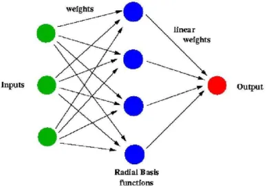
The Radial Basis Function (RBF) network (Figure 4.5) is the type of ANN employed in this work. The main features of RBF networks are:
- they are two-layer feed-forward networks;
- they are very good at interpolation;
- the output layer implements linear summation functions;
- the network training is divided into two stages: first the parameters of the hidden layer are determined, and then the weights from the hidden to output layer are obtained;
- both training and learning are very fast.
Figure 4.5: RBF network architecture.
Formally, a RBF network is a real-valued function whose value depends only on the distance from x to a point xi, called center, so that φ(x,xi) =
φ(kx−xik)3. Sums of radial basis functions are typically considered in
build-ing up function approximations of the form given by Equation 4.2, in which the approximating function y(x) is represented as a sum of N radial basis
functions, each one associated with a different centerxi, and weighted by an
appropriate coefficientwi. It can be shown that any continuous function on a 3
compact interval can in principle be interpolated with arbitrary accuracy by a sum of this form if a sufficiently large number N of radial basis functions is considered.
y(x) =
N X
i=1
wi· φ(kx−xik) (4.2)
In this work a common type of radial basis function is chosen: a Gaussian given by Equation 4.3,
φ(r) = exp
−r
2
σ2
, (4.3)
in whichr =kx−xikandσ is a parameter related to the spread of the
func-tion. Figure 4.6 presents an example of unidimensional Gaussian functions with xi = 0 and different σ values.
−4 −3 −2 −1 0 1 2 3 4
0 0.1 0.2 0.3 0.4 0.5 0.6 0.7 0.8 0.9 1
σ=1
σ=2
σ=3
Figure 4.6: Gaussian functions with σ = 1,2,3.
The RBF network possess three parameters: (i) the centers of the RBF functions (xi); (ii) the spread of the Gaussian RBF functions (σ), and (iii)
been proposed for training RBF networks. Generally, the training is divided into two stages. In the first stage (Steps 1 and 2) the number of radial basis functions and their parameters are determined based on unsupervised methods. In the second stage (Step 3) the adjustment of the weights from the hidden to the output layer is performed. Essentially this stage consists in finding the weights that optimize a single layer linear network.
The following techniques have been applied to train the RBF networks in each specified step.
Step 1 Finding the centers of the radial basis functions
- Initial methods, in which each data sample is assigned to a basis function [Specht,1990].
- Fixed centers selected at random [Broomhead and Lowe, 1988].
- K-means algorithm [Macqueen, 1967; Moody and Darken,1989].
- Adaptive k-means algorithm (self-organizing map) [Kohonen,1989].
- Subset selection [Berk, 1978; Chenet al., 1991]:
- forward selection: starts with an empty subset; added one basis function at a time (the one that most reduces the sum-squared-error); until some chosen criterion stops;
- backward elimination: starts with the full subset; removed one basis function at a time (the one that least increases the sum-squared-error); until some chosen criterion stops.
- Each value ofσis defined as the average of the Euclidean distances between the center of each sample and the center of the nearest sample [Moody and Darken, 1989].
- P-nearest neighbor algorithm (Equation4.4): a number P is cho-sen; for each center, the P nearest centers are found; the root-mean squared distance between the current cluster center and its P nearest neighbors is calculated [Knuth, 1998].
σj = v u u t1
P P X
i=1
(xj −xi)2 (4.4)
Step 3 Finding the weights from the hidden to the output layer
- Singular value decomposition (SVD) [Lay, 2002].
- Least Mean Squares (LMS) algorithm [Widrow and Hoff, 1988].
For the construction of the RBF network the MATLABc NEWRB
Name Value Name Value P Alternatives in the domain SPREAD 500
T Ranking of the alternatives MN 200
GOAL 0.1 DF 25
Table 4.1: MATLABc
parameters of the NEWRB function.
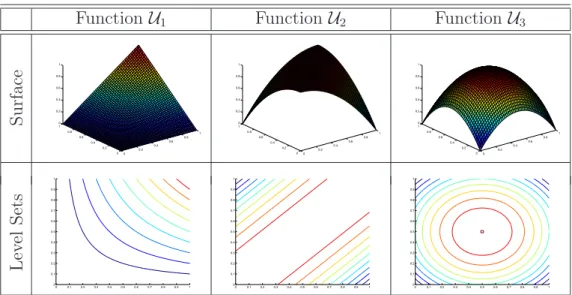
Underlying utility function Resulting estimated utility function S u rf ac e −2 −1 0 1 2 −2 −1 0 1 2 0 0.1 0.2 0.3 0.4 0.5 0.6 0.7 0.8 0.9 −2 −1 0 1 2 −2 −1 0 1 2 0 0.2 0.4 0.6 0.8 1 L ev el S et s
−2 −1.5 −1 −0.5 0 0.5 1 1.5 2 −2 −1.5 −1 −0.5 0 0.5 1 1.5 2
−2 −1.5 −1 −0.5 0 0.5 1 1.5 2 −2 −1.5 −1 −0.5 0 0.5 1 1.5 2
Figure 4.7: Surface and level sets of the functions U and ˆU.
−2 −1 0 1 2 −2 −1 0 1 2 0 0.2 0.4 0.6 0.8 1
It is not necessary to model U exactly because when the ranking is em-ployed in building the approximation the resulting function ˆU has level sets which are similar to the ones ofU and possesses information enough to codify the DM’s preferences. Therefore, the final surface is normalized by scaling the RBF output between 0 and 1. It is worth mentioning that any other interpolation method could have been chosen and the choice of the RBF net-work is due to its easy implementation and reduced computational load since the weights are updated linearly.
4.2.4
Step 4: Performance Assessment
Now that a model ˆU for the DM’s utility function U is available a value for each alternative can be inferred and a sorting of all alternatives can be constructed. This section presents a metric to assess the performance of the model ˆU related to the DM’s preferences.
The Kendall-tau Distance (KTD) [Kendall,1938] is a metric that counts the number of pairwise disagreements between two ranking lists. The KTD for a set A sorted according the rankings τ1 and τ2 is given by Equation 4.5.
K(τ1, τ2) = | {(i, j) :i < j,(τ1(i)< τ1(j)∧τ2(i)> τ2(j))
∨(τ1(i)> τ1(j)∧τ2(i)< τ2(j))} |. (4.5)
Consideringnthe list size, the normalized Kendall-tau distance, obtained by dividing the KTD value by n(n−1)/2 (total number of pairs), lies in the interval [0,1]. The normalized Kendall-tau distance, here simply represented by KTD, is employed in this work as the merit function.
Person A B C D E Sorting by height 1 2 3 4 5 Sorting by weight 3 4 1 2 5
Table 4.2: Example of the KTD metric.
The calculus of the Kendall-tau distance is made by comparing each pair of people and counting the number of discordant pairs, that is, the number of times where the values in the list L1 (height) are in the opposite order in
the list L2 (weight).
Pair Height Weight Discordant Pair (A, B) 1<2 3<4
(A, C) 1<3 3>1 X (A, D) 1<4 3>2 X (A, E) 1<5 3<5
(B, C) 2<3 4>1 X (B, D) 2<4 4>2 X (B, E) 2<5 4<5
(C, D) 3<4 1<2 (C, E) 3<5 1<5 (D, E) 4<5 2<5
Table 4.3: Concordant and discordant pairs.
As there are four pairs whose values are in the opposite order, the KTD value is 4. Normalizing this value, the resulting KTD, denoted τ, is τ = 0.4. The value τ = 0.4 indicates that there is a small similarity between the lists considered.
an absolute reference (the utility function U) is assumed to be available in the tests that have been performed. The KTD is a measure of the closeness between the sorting given by the resulting model and the optimal sorting provided by the DM.
In an attempt to assess the model’s performance, in each algorithm nvs = 30 validation sets with nvp = 50 randomly distributed alternatives are created in the domain D. The validation sets are constructed to evaluate the performance of the ˆU model within the entire domain D. A sorting for each validation set is obtained by the functions U and ˆU and the resulting KTD, also denotedτ, is the average of the obtained values of each validation set. A model is then said stable if τ satisfies a predefined tolerance tolst.
4.2.5
DM calls
This section presents an estimate of the number of queries required from the DM in the ranking procedure developed in Section 4.2.2. Let n be the number of alternatives in the set G and assume n = 2k, for some k ∈ N. In each step the pivot has to be compared with each alternative and, on average, the pivot splits the set in two sets with same size. That means in the first step the pivot is compared with n−1 alternatives, in the second step with n/2−1 alternatives, and the process goes on until only one alternative has left. As the expected number of levels is k = logn,4 the total number of
queries, denoted T(n), is given by Equation 4.6. 4