J. Braz. Chem. Soc. vol.19 número3

(1)

S

ho

rt

R

e

p

o

rt

*e-mail: [email protected]

Solubility Prediction of Solutes in Non-Aqueous Binary Solvent Mixtures

Abolghasem Jouyban,*

,a

_{Maryam Khoubnasabjafari,}

b

_{Somaieh Soltani,}

c

_{Shahla Soltanpour,}

d

Elnaz Tamizi

e

_{and William E. Acree Jr.}

f

a_{Faculty of Pharmacy and Drug Applied Research Center, Tabriz University of Medical Sciences, 51664, Iran}

b_{Kimia Research Institute, P.O. Box 51665-171, Iran}

c_{Research Center for Pharmaceutical Nanotechnology, Tabriz University of Medical Sciences, 51664, Iran}

d_{Biotechnology Research Centre, Tabriz University of Medical Sciences, 51664, Iran}

e_{Student Research Center, Tabriz University of Medical Sciences, 51664, Iran}

f_{Department of Chemistry, University of North Texas, Denton, TX 76203-5070, USA}

Foi investigada a possibilidade de substituir os parâmetros de Abraham calculados teoricamente pelos parâmetros experimentais, na previsão da solubilidade de solutos não-aquoso em misturas de solventes binários, utilizando-se o modelo de Jouyban-Acree. As solubilidades de 90 conjuntos de dados, coletados a partir da literatura, foram preditas utilizando-se estes parâmetros, os coeficientes de solventes e também as solubilidades de sistemas mono-solventes. A precisão das solubilidades previstas foi avaliada calculando-se a média percentual do desvio (MPD) e também dos desvios percentuais (IPDs) individuais. O MPD global para a análise utilizando os parâmetros de Abraham, experimentais e teóricos, foram os mesmos e <14%. Uma boa distribuição (IPD) foi obtida por estas análises numéricas. Os conjuntos de dados investigados neste trabalho foram coletados a várias temperaturas e os resultados confirmaram a possibilidade de previsão da solubilidade em solventes binários a diferentes temperaturas. Explorou-se a possibilidade de cálculos ab initio nesta previsão utilizando as solubilidades calculadas em sistemas mono-solventes. No entanto, a diferença entre os valores previstos e observados, para os coeficientes dos solventes, aumentou para aproximadamente 60% e 200% quando usou-se gás e água, respectivamente. Estes, são valores muito grandes para várias aplicações de previsão.

The possibility of replacing theoretically computed Abraham parameters with the experimental Abraham parameters in solubility prediction of solutes in non-aqueous binary solvent mixtures using the Jouyban-Acree model was investigated. The solubilities of 90 data sets collected from the literature were predicted using their Abraham parameters, the solvent coefficients and also the solubilities in mono-solvent systems. The accuracy of the predicted solubilities was evaluated by calculating the mean percentage deviation (MPD) and also individual percentage deviations (IPDs). The overall MPD for the analysis using experimental and computed Abraham parameters were the same and was < 14%. A favoured IPD distribution was obtained for these numerical analyses. The data sets investigated in this work were collected at various temperatures and the results confirmed the possibility of solubility prediction in binary solvents at various temperatures. We did explore the possibility of ab initio solubility prediction of solutes in binary mixtures using the calculated solubilities in mono-solvent systems, however, the difference between the predicted and observed values increased to ca. 60% for gas-to-solvent coefficients and ca.200% for water-to-solvent coefficients, which is too large for many predictive applications.

Keywords: solubility, prediction, non-aqueous mixed solvents, Abraham model, Jouyban-Acree model

Introduction

Solubility of a solute is affected by solvent’s and

(2)

Jouybanet al. 605 Vol. 19, No. 3, 2008

Abraham models employ five parameters for each solute and six solvent coefficients that were computed for a number of common solvents.3-4_{The basic models proposed for process} within condensed phases is:

(1)

and for process involving gas-to-condensed phase transfer is:

(2)

whereC_S and C_W are the solute solubility in the organic solvent and water (in mole per liter), respectively, C_G is the gas phase concentration of the solute, E is the excess molar refraction,S is dipolarity/polarizability of solute, Adenotes the solute’s hydrogen-bond acidity, B stands for the solute’s hydrogen-bond basicity, V is the McGowan volume of the solute, and L is the logarithm of the solute gas-hexadecane partition coefficient at 298.15 K. In equations (1) and (2) the coefficients c, e, s, a, b, v and l are the model constants (i.e. solvent’s coefficients), which depend upon the solvent system under consideration. Numerical values of the model constants have been reported in the literature3-4_for several water-to-organic solvent and gas-to-organic solvent systems.

Solvent mixing or cosolvency is the most common method to alter the solubility of a solute. There is an infinite number of solvent compositions for a given binary solvent, and for some compounds, both linear and non-linear solubility behavior have been reported in mixed solvent systems. The most accurate model to represent the solubility data in mixed solvent systems is the Jouyban-Acree model.7-9_{Its general form is:}

(3)

where X is the mole fraction solubility of the solute, f denotes the mole fraction of the solvents 1 and 2 in the solvent mixture, subscripts m, 1 and 2 are the mixed solvent and solvents 1 and 2, respectively, B_j is the model constant which represent various solute-solute, solvent-solvent and solute-solvent interactions. In a previous study,10_QSPR models were proposed to calculate the numerical values of theB_j terms using the Abraham coefficients for 22 solvents and solute descriptors for 5 solutes.

The QSPR models proposed in an earlier work using water-to-solvent coefficients were:

(4)

(5)

(6)

and the QSPR models using gas-to-solvent coefficients were:

(7)

(8)

(9)

The applicability of the proposed method was checked using 194 solubility data sets of five different solutes in various non-aqueous binary solvents. In this work, the possibility of replacing experimentally obtained Abraham parameters with the computed parameters is examined. The prediction capability of the previously developed QSPR models is checked using 90 solubility data sets11-24 of solutes which were not used in training process of the QSPR models. The applicability of the proposed method is also shown for predicting solubility at various temperatures. The main limitation of the Abraham model is that solute solvational parameters are known for only 4,000 organic compounds. In a recently released software25_{, this limitation} is overcome and one is able to compute E, S, A, B, V and Lparameters.

Computational Methods and Experimental

Data

The solubilities of the solutes in binary solvent mixtures were collected from the literature.11-24_{Table S1 listed details} of the experimental solubility data. The numerical values of the solvents’ coefficients were listed in Table S2. In addition to the experimental database of solute’s parameters, commercial software is also available to compute the parameters.25_{Table S3 lists the experimental and computed} values of solute’s parameters. Since the numerical values of A term for the solutes studied in the previous paper10_were equal to zero, the corresponding terms have been omitted from the QSPR models.

(3)

Solubility Prediction of Solutes in Non-Aqueous Binary Solvent Mixtures J. Braz. Chem. Soc. 606

of solutes in binary solvents. The predictions still required numerical values of the solute solubility in each pure solvent, i.e.X₁ and X₂. In order to provide a predictive model (without any experimentally determined data), C_S values of the solutes in the neat solvents under consideration were computed using Abraham models (using experimental values of C_W or C_G). The calculated molar solubilities, C_S, were converted to the mole fraction solubilities using density of the pure organic solvent. The calculated X₁ and X₂ values were then substituted into equation (3), along with theB_j values from equations (4)-(6) (or equations (7)-(9)) to predict the solubility in binary solvents by the Jouyban-Acree model. The density of pure organic solvents has been used to convert the molar solubility to mole fraction solubility and the effect of solute on density of the solution has been ignored. Table 1 summarizes the various numerical methods discussed in this work.

The predicitve ability of each computational method was assessed in terms of the mean percentage deviation (MPD) of observed ((X_m)_obs_.) and calculated ((X_m)_cal_.) solubilities, defined by equation (10):

(10)

whereN is the number of data points. In addition, we also calculated the individual percentage deviation (IPD):

(11)

for each solubility data point.

Results and Discussion

Validation of the previously derived coefficients for solubility predictions using computed Abraham solute descriptors

The solubilities of the solutes in 194 different binary solvent mixtures (for details see Table 1 of a previous paper10_{) were predicted using the Jouyban-Acree model} and calculated B_j values based on equations (4)-(6) and

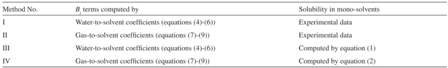
(7)-(9). Both experimental and computed Abraham solute descriptors were used in the B_j calculationss. Table 2 gives the overall MPD (± SD) values for the four predictive methods employed. There are no significant differences betweenMPDs for methods I and II that used experimental or computed Abraham parameters and experimental values ofX₁ and X₂ (t-test, p > 0.05). This observation is important in that it is possible to use computed solute descriptors instead of experimentally based values for predicting B_j constants of the Jouyban-Acree model. However, significant differences are observed using predicted X₁ and X₂ by equations (1) and (2) for the same set of data and the coefficients (p < 0.0005), revealing that the computed Abraham parameters using PharmaAlgorithm software produced less accurate solubility predictions in mono-solvent systems in comparison with the experimental Abraham parameters. To confirm this hypothesis, readers could refer to the predicted solubilities using equations (1) and (2) employing experimental Abraham parameters. As examples, the IPDs of the predicted solubilities of anthracene using equation (1) in various solvents were listed in Table S4 where the differences between predicted solubilities using experimental and computed Abraham parameters were statistically significant (paired t-test, p < 0.001 or p < 0.0005, for details see footnote of Table 1. Details of various numerical analyses carried out using experimental and computed Abraham parameters

Method No. Bj terms computed by Solubility in mono-solvents

I Water-to-solvent coefficients (equations (4)-(6)) Experimental data

II Gas-to-solvent coefficients (equations (7)-(9)) Experimental data

III Water-to-solvent coefficients (equations (4)-(6)) Computed by equation (1)

IV Gas-to-solvent coefficients (equations (7)-(9)) Computed by equation (2)

Table 2. Overall MPD (±SD) for solubility prediction of 194 sets from a previous work,10_{and this work using experimental and computed Abraham} solute parameters

Numerical method

Experimental parameters

Computed parameters

Significance

194 data set from a previous work

I 4.6 ± 3.9 4.6 ± 4.0 Not significant

II 11.3 ± 13.3 10.5 ± 13.0 Not significant

III 33.0 ± 20.6 52.0 ± 32.2 p < 0.0005

IV 23.9 ± 21.5 118 ± 258.4 p < 0.0005

This work

I 13.7 ± 14.0 13.6 ± 13.8 Not significant

II 12.7 ± 13.9 12.5 ± 13.7 Not significant

III 228.4 ± 337.7 168.8 ± 325.4 Not significant

(4)

Table S4). A possible reason for such deviations could be the non-ideally adjusted water-to-solvent coefficients of some solvents as it was reported slightly different c, e, s, a, b and v values for cyclohexane in an earlier report1_and a recent one5_{in which the IPD of anthracene solubility in} cyclohexane predicted by equation (1) using earlier1_and amended5_{c, e, s, a, b and v values were 213.2 and 148.4%,} respectively. We have computed the IPD of anthracene in cyclohexane using amended5_{c, e, s, a, b and v values equal} to 149.6%. The second reason for very large deviations between theoretically derived and experimentally determined solubility values could be any error in the solute’s parameter calculations. The third reason could be the temperature effects on X₁ and X₂ values which did not considered in the equations (1) and (2).

It is possible to improve our ab initio prediction approach by developing better methods to predict the solubility in mono-solvent systems. It is difficult to guesstimate the error that one could reasonably expect from employing predictive methods to estimate the solubility in the neat organic solvents as the published methods have been tested on relatively few of the many possible solute-solvent combinations. Based on our review of the published comparisons, we do not think that it would be unreasonable to assign an expected error in the range of 0.1 to 0.3 log units to solubilities predicted by group contribution and linear free energy correlations for many of the simpler systems.

Predictions using water-to-solvent process and experimental solubility data in mono-solvents

The predictive calculations discussed in the preceding section concerned solubility data used in generating equations (4)-(9). A more stringent test of any predictive solubility method is its ability to accurately predict solubilities of additional solute molecules, or solubilities of solutes dissolved in additional binary solvent mixtures. To better assess the applications and limitations of methods I-IV, we have compiled from the published literature experimental solubility data for 90 additional data sets (see Table S1). In the first set of calculations on the new data set, we computed the B_j coefficients using equations (4)-(6) and experimentally-based Abraham solute descriptors. The calculated B_j values were then combined with experimentally measured solubility data in the mono-solvents to predict the mole fraction solubility lnX_m values for the 90 additional data sets (numerical method I of Table 1) using equation (3). The prediction accuracy of the data was evaluated using MPD values for this analysis and reported in column 2 of Table S5. The

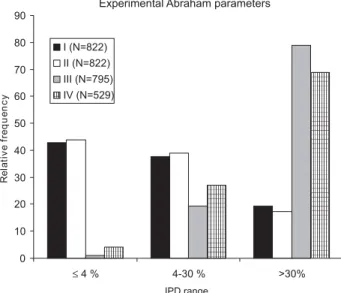
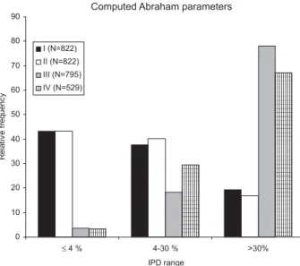
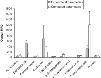
minimum (0.2%) and maximum (61.6%) MPDs were observed for p-benzoquinone in 2, 2, 4-trimethylpentane + cyclohexane and benzophenone in carbon tetrachloride + dodecane mixtures both at 25 nC. The overall MPD(± SD) was 13.7 ± 14.0%. A similar set of calculations were performed using computed Abraham parameters by PharmaAlgorithm software (see column 6 of Table S5). The minimum (0.2%) and maximum (61.8%) MPDs were observed for the same data sets and the overall MPD (± SD) was 13.6 ± 13.8%. There was no significant difference between 13.7 and 13.6% (paired t-test, p > 0.05). Figures 1 and 2 showed the relative frequencies of IPDs sorted in three subgroups, i.e.a 4, 4-30 and > 30%, for various numerical methods employing experimental and computed Abraham parameters. There was no significant difference between frequencies of IPDs of both parameters for numerical method I. Figure S1 depicted the overall MPDs for various solutes and there was no difference between MPDs calculated using experimental and computed Abraham parameters. These findings confirm the above results using 194 data sets from a previous work10 and reveal that it is possible to replace the experimentally determined Abraham parameters with the computationally obtained parameters for solubility prediction in mixed solvent system using method I.

The equations (4)-(6) were obtained employing the B_j terms calculated using solubility data of solutes at 25 and 26 nC, however, the equations were able to predict the solubility a wider temperature range (20-50 nC) as is evident (as examples) from set numbers 1-7 or 8-14 of Table S1. This is an oversimplification on the constants of the Jouyban-Acree model where it has been assumed that

(5)

the Jouyban-Acree model constants are not temperature dependent. The reason for this simplification was the shortage of the solubility data of solutes in non-aqueous binary solvents at various temperatures. The capability of the Jouyban-Acree model for calculating the solubility of solutes in binary solvents at various temperatures has been shown earlier.26

Predictions using gas-to-solvent process and experimental solubility data in mono-solvents

In the second set of calculations on the new data set, we computed the B_j coefficients using equations (7)-(9) and experimentally-based Abraham solute descriptors. The calculated B_j values were then combined with experimental lnX₁ and lnX₂ data to predict the mole fraction solubility lnX_m values for the 90 additional data sets (numerical method II of Table 1) using equation (3). The obtained MPD values are reported in column 3 of Table S5. The minimum (0.2%) and maximum (67.3%) MPDs were observed for p-benzoquinone in heptane + cyclohexane and for benzophenone in carbon tetrachloride + dodecane mixtures both at 25 nC. The overall MPD (± SD) was 12.7 ± 13.9%. The same calculations were carried out using the computed Abraham parameters by PharmaAlgorithm software and theMPDs were listed in the column 7 of Table S5). The minimum (0.2%) and maximum (68.4%) MPDs were observed for p-benzoquinone in heptane + cyclohexane and benzophenone in carbon tetrachloride + dodecane mixtures and the overall MPD (± SD) was 12.5 ± 13.7%. There were i) no significant difference between 12.7 and 12.5% (pairedt-test, p >0.05), ii) the same frequency pattern for

bothIPDs and iii) no difference between overall MPDs for various solutes (see Figure S2) employing experimental and computed Abraham parameters, revealing that one can employ solute parameters computed by PharmaAlgorithm instead of their experimentally obtained values. Full agreement was observed from the results of the 90 and 194 data sets (see Table 2) and the relative frequency of IPDs was favorable.

Ab initio predictions using water-to-solvent process and computed solubility data in mono-solvents

In the third set of predictive calculations we again calculated the B_j terms using equations (4)-(6) and the experimentally-based Abraham solute descriptors; however, in equation (3) the experimental mole fraction solubilities in the two mono-solvents were replaced with estimated X₁ and X₂ values based on equation (1). Results of these calculations are summarized in the fourth column of Table S5 for 86 of the 90 data sets considered. Predictions could not be made for the four p-tolylacetic acid systems because the molar solubility of p-tolylacetic acid in water, C_w, was not known. The molar solubility of the solute in water is a required input parameter in the estimation of solute’s solubility in mono-solvents through equation (1). A minimum MPD of 11.2% was observed for naphthalene in benzene + toluene at 25 nC, and a maximum MPD of 1811.2% was obtained for carbazole in octane + cyclohexane at 25 nC. The overall average MPD was 228.7%. The largest MPDs were observed for data set numbers 15-22 (benzoic acid), 29-44 (carbazole) and 77-82 (phenylacetic acid). Similar computations were performed using computed Abraham parameters for predicting X₁,X₂ andB

j terms using the relevant equations. The MPD values

of these computations are listed in column 8 of Table S5. A nearly identical MPD pattern was observed for data predicted by the experimental and computed parameters. The overall MPD was 168.9%. Figure S3 showed overall MPD for various solutes studied for experimental and computed parameters. This particular estimational scheme (method III) requires a prior knowledge of the solute’s aqueous molar solubility, and based on the relatively large IPD and MPD between predicted and observed values the method did not provide a very reasonable prediction of the observed solubility behavior.

Ab initio predictions using gas-to-solvent process and computed solubility data in mono-solvents

Numerical method IV (see Table 1) involved using B_j coefficiens based on equations (7)-(9), and estimated Figure 2. The relative frequency of the individual percentage deviations

(6)

values for the solubility of the solute in both mon-solvents computed from equation (2). The minimum and maximum MPD for method IV (see column 5 of Table S5) were 3.6 and 101.5%, respectively, for naphthalene dissolved in benzene + toluene at 25 nC and for pyrene dissolved in toluene + heptane at 20 nC using experimentally-based Abraham solute descriptors. The overall MPD was 53.5 (± 30.0)%. A slightly larger minimum MPD of 5.6% (for naphthalene in carbon tetrachloride + hexane) and larger maximum MPD of 197.5% (for pyrene in toluene + heptane at 20 nC) were obtained using computed Abraham solute descriptors. The overall MPD was also larger, MPD = 62.7%, for the method IV predictions that used computed solute descriptors as input values (see column 9 of Table S5). As discussed above, the large deviations in binary solvents result mostly from the high IPDs of the solutes in mono-solvents (see Table S6 for details). It is difficult to accurately predict solubility in binary solvent mixtures when the inputted solubility data for the mono-solvents that make up the binary solvent mixtures is poorly predicted. Better estimation methods for solute solubility in mono-solvents should allow one to reduce these deviations significantly.

Conclusions

Published methods for estimating the B_j constants of the Jouyban-Acree model were applied successfully to a data set containing experimental solubility data for 90 additional solute-binary solvent-temperature combinations. None of the binary solvent solubility data was used in the regression analyses used to develop the predictive B_j correlations. The predicted B_j constants, when combined with experimental solubility data for the solute dissolved in the mono-solvents, enabled one to estimate the solubility of crystalline organic solutes in binary solvents using the Jouyban-Acree model. The expected prediction errors were < 14 and < 13%, respectively for water-to-solvent and gas-to-solvent coefficients employing both experimentally determined and theoretically calculated Abraham solute descriptors. The relatively small prediction errors indicate that it is possible to predict the solubility in binary solvents with minimum experimental efforts. Experimental solubility data exists in the published literature for many organic solutes in mono-solvents, and the Jouyban-Acree model allows one to quantitively estimate the extent to which cosolvency increases or decreases solute solubility. Such predictions are important in both solubilization and crystallization processes. Moreover, predictive methods, such as the Jouyban-Acree model, provide a convenient means to screen compiled experimental solubility data

in order to detect possible outliers for re-determination. For any solubility datum with very high IPD, the re-measurement is recommended. The proposed methods could also be extended to predict the solubility in mixed solvents at various temperatures. We tried to develop an ab initio prediction method employing C_W or C_G data of the solute (numerical methods III and IV); however, the obtainedMPDs were ca. 200 and 60%.

As a practical conclusion, there are a number of possible solutions depending on the availability of the required input data:i) If the experimental solubility data of the solute in mono-solvent systems, i.e. X₁ and X₂, are available, the best solution to predict the solubility in mixed solvents is the numerical methods I or II and the expected prediction error is ca. 14%. ii) If X₁ and X₂ are not available and the aqueous solubility of the solute is known, one could use the numerical method III and the expected prediction error is relatively high (170%) for computed Abraham parameters. iii) If X₁ and X₂ are not available and C_G of the solute is known, the numerical method IV could be a solution and the expected prediction error is slightly high (ca. 60%) for computed Abraham parameters.

Supplemenatry Information

Supplementary data are available free of charge at http://jbcs.sbq.org.br, as PDF file.

Acknowledgments

The financial support from Drug Applied Research Center (under grant number 85-64) was gratefully acknowledged. The authors also thank PharmaAlgorithm Inc. for the trial version of their software.

References

1. Abraham, M. H.; Green, C. E.; Acree, Jr., W. E.; Hernandez, C. E.; Roy, L. E.; J. Chem. Soc., Perkin Trans. 1998,2, 2677. 2. Acree, Jr., W. E.; Abraham, M. H.; Can. J. Chem.2001,79,

1466.

3. Stovall, D. M.; Acree, Jr., W. E.; Abraham, M. H.; Fluid Phase

Equilib.2005,232, 113.

4. Stovall., D. M.; Givens, C.; Keown, S.; Hoover, K. R.; Barnes, R.; Harris, C.; Lozano, J.; Nguyen, M.; Rodriguez, E.; Acree, Jr., W.E.; Abraham, M.H.; Phys. Chem. Liq. 2005,43, 351. 5. Acree, Jr.,W. E.; Abraham, M. H.; Fluid Phase Equilib. 2002,

201, 245.

6. Acree, Jr., W. E.; Abraham, M. H.; J. Solution Chem. 2002,31, 293.

(7)

8. Jouyban-Gharamaleki, A.; Valaee, L.; Barzegar-Jalali, M.; Clark, B.J. Acree, Jr., W.E.; Int. J. Pharm. 1999,177, 93. 9. Jouyban, A.; Chan, H.K.; Chew, N. Y. K.; Khoubnasabjafari,

M.; Acree, Jr., W. E.; Chem. Pharm. Bull. 2006,54, 428. 10. Jouyban, A.; Acree, Jr., W. E.; Fluid Phase Equilib. 2006,249,

24.

11. Al-Sharrah, G.K.; Ali, S.H.; Fahim, M.A.; Fluid Phase Equilib. 2002,193, 191

12. Acree, Jr., W.E.; Bertrand, G.L.; J. Pharm. Sci.1981,70, 1033.

13. Azizian, S.; Haydarpour, A.; J. Chem. Eng. Data2003, 48, 1476.

14. Acree, Jr., W.E.; Phys. Chem. Liq.1990,22, 157.

15. McCargar, J.W.; Acree, Jr., W.E.; Phys. Chem. Liq.1987,17, 123.

16. Acree, Jr., W.E.; Tucker, S.A.; Int. J. Pharm.1993,101, 199. 17. McCargar, J.W.; Acree, Jr., W.E.; J. Pharm. Sci. 1987,76,

572.

18. Heric, E.L.; Posey, C.D.; J. Chem. Eng. Data1964,9, 35. 19. Heric, E.L.; Posey, C.D.; J. Chem. Eng. Data1965,10, 25. 20. Heric, E.L.; Posey, C.D.; J. Chem. Eng. Data1964,9, 161. 21. Acree, Jr., W.E.; Rytting, J.H.; J. Pharm. Sci.1982,10, 231.

22. Judy, C.L.; Acree, Jr., W.E.; Int. J. Pharm.1985,27, 39. 23. Ali, S.H.; Al-Mutairi, F.S.; Fahim, M.A.; Fluid Phase Equilib.

2005,230, 176.

24. Acree, Jr., W.E.; J. Chem. Eng. Data1985,30, 70.

25. P h a r m a A l g o r i t h m s , A D M E B o x e s , Ve r s i o n 3 . 0 , PharmaAlgorithms Inc., 591 Indian Road, Toronto, ON M6P 2C4, Canada, 2006.

26. Jouyban, A.; Acree, Jr., W. E.; Fluid Phase Equilib. 2003,209, 155.

27. Abraham, M.H.; Zissimos, A.M.; Acree Jr., W.E.; Phys. Chem.

Chem. Phys. 2001,3, 3732.

28. Abraham, M.H.; Le, J.; J. Pharm. Sci.1999,88, 868. 29. Yalkowsky, S.H.; Valvani, S.C.; J. Pharm. Sci. 1980,69, 912. 30. Abraham, M.H.; Le, J.; Acree, W.E.; Carr, P.W.; Dallas, A.J.;

Chemosphere. 2001,44, 855.

31. Yalkowsky, S.H.; He, Y.; Handbook of aqueous solubility data, CRC press, Florida, 2003.

32. Monte, M.J.S.; Hillesheim, D.M.; J. Chem. Eng. Data2001, 46, 1601.

Received: August 23, 2007

(8)

S

u

p

le

m

e

nta

ry

Inf

o

rm

a

ti

o

n

*e-mail: [email protected]

Solubility Prediction of Solutes in Non-Aqueous Binary Solvent Mixtures

Abolghasem Jouyban,*

,a

_{Maryam Khoubnasabjafari,}

b

_{Somaieh Soltani,}

c

_{Shahla Soltanpour,}

d

Elnaz Tamizi

e

_{and William E. Acree Jr.}

f

a_{Faculty of Pharmacy and Drug Applied Research Center, Tabriz University of Medical Sciences, 51664, Iran}

b_{Kimia Research Institute, P.O. Box 51665-171, Iran}

c_{Research Center for Pharmaceutical Nanotechnology, Tabriz University of Medical Sciences, 51664, Iran}

d_{Biotechnology Research Centre, Tabriz University of Medical Sciences, 51664, Iran}

e_{Student Research Center, Tabriz University of Medical Sciences, 51664, Iran}

f_{Department of Chemistry, University of North Texas, Denton, TX 76203-5070, USA}

Figure S3. The overall MPD (± SD) for numerical method III for various

solutes

Figure S2. The overall MPD (± SD) for numerical method II for various

solutes

Figure S1. The overall MPD (± SD) for numerical method I for various

(9)

Solubility Prediction of Solutes in Non-Aqueous Binary Solvent Mixtures J. Braz. Chem. Soc.

S2

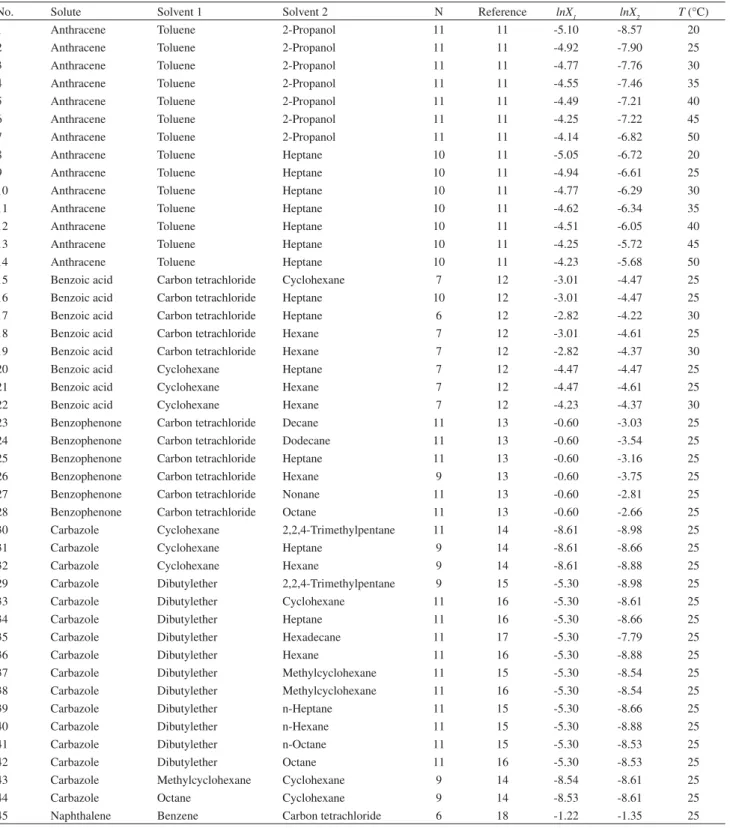
Table S1. Details of solutes and solvents names, the references of experimental data sets, logarithms of solubility in mono-solvents (lnX₁ and lnX₂) and

temperature (T)

No. Solute Solvent 1 Solvent 2 N Reference lnX₁ lnX₂ T (nC)

1 Anthracene Toluene 2-Propanol 11 11 -5.10 -8.57 20

8 Anthracene Toluene Heptane 10 11 -5.05 -6.72 20

15 Benzoic acid Carbon tetrachloride Cyclohexane 7 12 -3.01 -4.47 25

16 Benzoic acid Carbon tetrachloride Heptane 10 12 -3.01 -4.47 25

17 Benzoic acid Carbon tetrachloride Heptane 6 12 -2.82 -4.22 30

18 Benzoic acid Carbon tetrachloride Hexane 7 12 -3.01 -4.61 25

19 Benzoic acid Carbon tetrachloride Hexane 7 12 -2.82 -4.37 30

20 Benzoic acid Cyclohexane Heptane 7 12 -4.47 -4.47 25

21 Benzoic acid Cyclohexane Hexane 7 12 -4.47 -4.61 25

22 Benzoic acid Cyclohexane Hexane 7 12 -4.23 -4.37 30

23 Benzophenone Carbon tetrachloride Decane 11 13 -0.60 -3.03 25

24 Benzophenone Carbon tetrachloride Dodecane 11 13 -0.60 -3.54 25

25 Benzophenone Carbon tetrachloride Heptane 11 13 -0.60 -3.16 25

26 Benzophenone Carbon tetrachloride Hexane 9 13 -0.60 -3.75 25

27 Benzophenone Carbon tetrachloride Nonane 11 13 -0.60 -2.81 25

28 Benzophenone Carbon tetrachloride Octane 11 13 -0.60 -2.66 25

30 Carbazole Cyclohexane 2,2,4-Trimethylpentane 11 14 -8.61 -8.98 25

31 Carbazole Cyclohexane Heptane 9 14 -8.61 -8.66 25

32 Carbazole Cyclohexane Hexane 9 14 -8.61 -8.88 25

29 Carbazole Dibutylether 2,2,4-Trimethylpentane 9 15 -5.30 -8.98 25

33 Carbazole Dibutylether Cyclohexane 11 16 -5.30 -8.61 25

34 Carbazole Dibutylether Heptane 11 16 -5.30 -8.66 25

35 Carbazole Dibutylether Hexadecane 11 17 -5.30 -7.79 25

36 Carbazole Dibutylether Hexane 11 16 -5.30 -8.88 25

37 Carbazole Dibutylether Methylcyclohexane 11 15 -5.30 -8.54 25

38 Carbazole Dibutylether Methylcyclohexane 11 16 -5.30 -8.54 25

39 Carbazole Dibutylether n-Heptane 11 15 -5.30 -8.66 25

40 Carbazole Dibutylether n-Hexane 11 15 -5.30 -8.88 25

41 Carbazole Dibutylether n-Octane 11 15 -5.30 -8.53 25

42 Carbazole Dibutylether Octane 11 16 -5.30 -8.53 25

43 Carbazole Methylcyclohexane Cyclohexane 9 14 -8.54 -8.61 25

44 Carbazole Octane Cyclohexane 9 14 -8.53 -8.61 25

(10)

Jouybanet al. S3 Vol. 19, No. 3, 2008

Table S1. continuation

No. Solute Solvent 1 Solvent 2 N Reference lnX₁ lnX₂ T (nC)

46 Naphthalene Benzene Cyclohexane 8 18 -1.22 -1.91 25

47 Naphthalene Benzene Hexadecane 6 18 -1.22 -1.59 25

48 Naphthalene Benzene Hexane 8 18 -1.22 -2.15 25

49 Naphthalene Benzene Toluene 7 18 -1.22 -1.23 25

50 Naphthalene Carbon tetrachloride Cyclohexane 6 19 -1.35 -1.91 25

51 Naphthalene Carbon tetrachloride Hexadecane 6 19 -1.35 -1.59 25

52 Naphthalene Carbon tetrachloride Hexane 8 19 -1.35 -2.15 25

53 Naphthalene Cyclohexane Hexane 6 19 -1.91 -2.15 25

54 Naphthalene Hexadecane Cyclohexane 7 19 -1.59 -1.91 25

55 Naphthalene Hexadecane Hexane 6 19 -1.59 -2.15 25

56 Naphthalene Toluene Carbon tetrachloride 6 20 -1.23 -1.35 25

57 Naphthalene Toluene Cyclohexane 6 20 -1.23 -1.91 25

58 Naphthalene Toluene Hexadecane 6 20 -1.23 -1.59 25

59 Naphthalene Toluene Hexane 6 20 -1.23 -2.15 25

60 p-Benzoquinone 2,2,4-Trimethylpentane Cyclohexane 7 21 -5.01 -5.03 25

61 p-Benzoquinone Carbon tetrachloride Heptane 8 21 -3.37 -5.01 25

62 p-Benzoquinone Carbon tetrachloride Octane 7 21 -3.37 -4.89 25

63 p-Benzoquinone Dodecane Heptane 7 21 -4.74 -5.01 25

64 p-Benzoquinone Heptane Cyclohexane 7 21 -5.01 -5.03 25

65 p-Tolylacetic acid Cyclohexane 2,2,4-Trimethylpentane 7 22 -4.32 -4.83 25

66 p-Tolylacetic acid Cyclohexane Heptane 7 22 -4.30 -4.78 25

67 p-Tolylacetic acid Cyclohexane Hexane 8 22 -4.32 -4.85 25

68 p-Tolylacetic acid Cyclohexane Octane 7 22 -4.32 -4.75 25

69 Phenanthrene Toluene 2,2,4-Trimethylpentane 7 23 -0.77 -3.96 20

73 Phenanthrene Toluene Heptane 11 23 -0.77 -4.17 20

77 Phenylacetic acid Carbon tetrachloride 2,2,4-Trimethylpentane 11 24 -1.75 -4.40 25

78 Phenylacetic acid Carbon tetrachloride Cyclohexane 11 24 -1.75 -3.70 25

79 Phenylacetic acid Carbon tetrachloride Heptane 11 24 -1.75 -4.31 25

80 Phenylacetic acid Carbon tetrachloride Octane 11 24 -1.75 -4.24 25

81 Phenylacetic acid Cyclohexane 2,2,4-Trimethylpentane 9 24 -3.70 -4.40 25

82 Phenylacetic acid Cyclohexane Heptane 8 24 -3.70 -4.31 25

83 Pyrene Toluene 2,2,4-Trimethylpentane 12 20 -2.87 -4.72 20

87 Pyrene Toluene Heptane 11 20 -2.87 -4.47 20

(11)

S4

Table S2. Coefficients in equations (1) and (2) for water-to-solvent and gas-to-solvent processes of the solvents used in this studya

No. Water-to-solvent coefficients c e s a b v

1 2,2,4-Trimethylpentane 0.288 0.382 -1.668 -3.639 -5.000 4.461

2 2-Propanol 0.063 0.320 -1.024 0.445 -3.824 4.067

3 Benzene 0.142 0.464 -0.588 -3.099 -4.625 4.491

4 Carbone tetrachloride 0.260 0.573 -1.254 -3.558 -4.558 4.589

5 Cyclohexane 0.159 0.784 -1.678 -3.740 -4.929 4.577

6 Decane 0.160 0.585 -1.730 -3.440 -5.080 4.582

7 Dibutyl ether 0.203 0.369 -0.954 -1.488 -5.426 4.508

8 Dodecane 0.114 0.668 -1.640 -3.550 -5.010 4.459

9 Heptane 0.325 0.670 -2.061 -3.317 -4.733 4.543

10 Hexadecane 0.087 0.667 -1.620 -3.59 -4.870 4.433

11 Hexane 0.361 0.579 -1.723 -3.599 -4.764 4.344

12 Methylcyclohexane 0.246 0.782 -1.982 -3.517 -4.293 4.528

13 Nonane 0.240 0.619 -1.710 -3.530 -4.920 4.482

14 Octane 0.223 0.642 -1.647 -3.480 -5.067 4.526

15 Toluene 0.143 0.527 -0.720 -3.010 -4.824 4.545

No. Gas-to-solvent coefficients c e s a b l

1 2,2,4-Trimethylpentane 0.275 −0.244 0.000 0.000 0.000 0.972

2 2-Propanol -0.060 -0.335 0.702 4.017 1.040 0.893

3 Benzene 0.107 −0.313 1.053 0.457 0.169 1.020

4 Carbone tetrachloride 0.282 −0.303 0.460 0.000 0.000 1.047

5 Cyclohexane 0.163 -0.110 0.000 0.000 0.000 1.013

6 Decane 0.156 -0.140 0.000 0.000 0.000 0.989

7 Dibutyl ether 0.165 −0.421 0.760 2.102 −0.664 1.002

8 Dodecane 0.053 0.000 0.000 0.000 0.000 0.986

9 Heptane 0.275 −0.162 0.000 0.000 0.000 0.983

10 Hexadecane 0.000 0.000 0.000 0.000 0.000 1.000

11 Hexane 0.292 −0.169 0.000 0.000 0.000 0.979

12 Methylcyclohexane 0.318 −0.215 0.000 0.000 0.000 1.012

13 Nonane 0.200 -0.145 0.000 0.000 0.000 0.980

14 Octane 0.215 −0.049 0.000 0.000 0.000 0.967

15 Toluene 0.121 −0.222 0.938 0.467 0.099 1.012

a_{Data taken from a reference.}5

Table S3. The experimental and computed Abraham parameters along with the input properties for solutes studied in this work and their references

Solute E S A B V L logC_W logC_G Reference

Experimental Abraham parameters

Anthracene 2.290 1.34 0.000 0.280 7.568 -6.430 -9.460 2

Benzoic acid 0.730 0.90 0.590 0.400 4.395 -1.550 -6.690 27

Benzophenone 1.447 1.50 0.000 0.500 6.852 -3.12028 _-a ₂₅

Carbazole 1.787 2.01 0.180 0.080 7.982 -5.27028 _-a ₂₅

Naphthalene 1.340 0.92 0.000 0.200 5.161 -3.61029 _-5.340 ₃₀

p-Benzoquinone 0.750 0.55 0.000 0.810 3.492 -0.88031 _-a ₂₅

p-Tolylacetic acid 0.730 0.97 0.600 0.640 5.480 -a _-a ₂₅

Phenanthrene 2.055 1.29 0.000 0.290 7.632 -5.170 -7.970 2

Phenylacetic acid 0.730 1.01 0.590 0.610 4.933 -0.89028 _-7.562b ₂₅

Pyrene 2.808 1.71 0.000 0.280 8.833 -6.150 -9.650 5

Computed Abraham parameters

Anthracene 1.99 1.34 0.000 0.23 1.454 7.706 25

Benzoic acid 0.75 1.08 0.570 0.44 0.932 4.533 25

Benzophenone 1.37 1.59 0.000 0.51 1.481 7.308 25

Carbazole 1.94 1.43 0.310 0.39 1.315 7.869 25

Naphthalene 1.27 1.02 0.000 0.17 1.085 5.332 25

p-Benzoquinone 0.90 0.43 0.000 0.76 0.791 3.500 25

p-Tolylacetic acid 0.77 1.02 0.570 0.45 1.214 5.499 25

Phenanthrene 1.99 1.34 0.000 0.23 1.454 7.706 25

Phenylacetic acid 0.75 1.08 0.570 0.45 1.073 5.028 25

Pyrene 2.60 1.52 0.000 0.25 1.585 9.110 25

a_{The data was not available.}

b_logC

G of phenylacetic acid was calculated using the extrapolated vapor pressure data from a reference

(12)

Jouybanet al. S5 Vol. 19, No. 3, 2008

Table S4. The individual percentage deviations (IPDs) of solubilities of solutes10_{in some of the solvents predicted by equations (1) and (2) employing}

experimental and computed Abraham parameters

Solutea _Solventa T (nC) Experimental parameters Computed parameters

Equation (1) Equation (2) Equation (1) Equation (2)

Anthracene 1,4-Dioxane 25 20.5 20.0 64.4 36.1

Anthracene 1-Butanol 25 25.5 1.0 45.6 43.7

Anthracene 1-Octanol 25 17.0 23.9 35.7 8.8

Anthracene 1-Pentanol 25 34.4 21.9 47.0 13.5

Anthracene 2,2,4-Trimethylpentane 25 40.3 36.3 18.5 2.6

Anthracene 2-Butanol 25 21.2 24.0 55.6 22.8

Anthracene 2-Methyl-1-propanol 25 37.7 11.7 64.8 34.1

Anthracene 2-Propanol 25 28.5 5.4 60.0 40.4

Anthracene Acetonitrile 25 14.6 6.3 80.0 70.1

Anthracene Benzene 25 97.7 52.7 143.6 155.2

Anthracene Carbon tetrachloride 25 49.3 3.3 69.7 65.7

Anthracene Cyclohexane 25 149.6 7.7 156.1 37.3

Anthracene Dibutyl ether 25 11.5 32.4 61.2 33.8

Anthracene Heptane 25 16.7 28.2 9.6 9.7

Anthracene Hexane 25 12.0 26.2 2.0 13.2

Anthracene Methanol 25 3.2 1.8 24.0 27.9

Anthracene Methyl tert-buthyl ether 25 22.6 24.6 82.0 44.6

Anthracene Methylcyclohexane 25 66.8 17.8 59.4 31.4

Anthracene Octane 25 46.8 18.7 68.8 14.3

Anthracene Toluene 25 132.9 78.7 181.0 182.0

Benzil 1-Butanol 25 5.3 15.8 94.8 1599.5

Benzil 1-Octanol 25 60.1 29.0 91.8 1540.8

Benzil 1-Pentanol 25 10.9 95.6 95.1 1421.3

Benzil 1-Propanol 25 5.7 25.1 94.9 1146.8

Benzil 2,2,4-Trimethylpentane 25 38.2 29.4 99.0 375.6

Benzil 2-Butanol 25 46.5 32.3 91.0 2172.1

Benzil 2-Propanol 25 25.4 14.0 92.6 1882.9

Benzil Carbon tetrachloride 25 38.6 51.6 97.8 337.6

Benzil Cyclohexane 25 4.2 36.7 98.0 373.9

Benzil Heptane 25 34.2 10.9 99.1 521.9

Benzil Octane 25 25.6 14.2 97.7 498.8

Pyrene 1-Butanol 26 33.8 42.0 17.2 115.8

Pyrene 1-Octanol 26 39.8 1.9 0.0 45.3

Pyrene 1-Pentanol 26 34.0 43.1 18.1 16.8

Pyrene 1-Propanol 26 21.2 13.8 35.0 26.1

Pyrene 2,2,4-Trimethylpentane 26 75.4 23.1 40.1 59.7

Pyrene 2-Butanol 26 36.8 2.8 11.0 50.2

Pyrene 2-Methyl-1-propanol 26 26.4 21.0 29.4 77.3

Pyrene 2-Propanol 26 27.7 41.5 26.2 100.7

Pyrene Benzene 26 64.4 210.3 124.4 300.3

Pyrene Cyclohexane 26 59.5 38.1 215.3 173.6

Pyrene Dibutyl ether 26 32.0 9.7 23.6 86.4

Pyrene Heptane 26 66.0 5.7 16.1 88.8

Pyrene Hexane 26 57.4 0.0 5.2 100.7

Pyrene Methylcyclohexane 26 25.8 1.2 61.5 105.9

Pyrene Octane 26 23.5 8.7 62.1 103.4

Thianthrene 2,2,4-Trimethylpentane 25 45.2 27.1 71.1 112.5

Thianthrene Cyclohexane 25 53.1 22.9 29.4 121.9

Thianthrene Heptane 25 12.3 3.1 56.2 176.4

Thianthrene Hexane 25 17.7 12.6 58.4 149.3

(13)

S6

Solutea _Solventa T (nC) Experimental parameters Computed parameters

Equation (1) Equation (2) Equation (1) Equation (2)

Thianthrene Octane 25 57.1 7.7 25.1 189.8

Trans-Stilbene 1-Propanol 25 23.4 10.8 33.9 57.4

Trans-Stilbene 2,2,4-Trimethylpentane 25 22.2 9.5 16.7 63.0

Trans-Stilbene 2-Butanol 25 53.2 28.5 79.9 32.5

Trans-Stilbene Cyclohexane 25 32.2 14.5 22.7 67.7

Trans-Stilbene Heptane 25 6.0 5.4 23.9 62.6

Trans-Stilbene Hexane 25 17.7 8.7 22.0 63.7

Trans-Stilbene Methylcyclohexane 25 21.4 4.3 8.8 62.5

Trans-Stilbene Octane 25 27.2 11.9 27.5 65.9

Anthracene 1,4-Dioxane 25 20.5 20.0 64.4 36.1

All 36.3b _24.4c _59.7b _262.8c

25 34.6d _22.2e _64.5d _319.4e

a_{Details of the references of data were reported in an earlier work.}10_;b7KHGLIIHUHQFHZDVVWDWLVWLFDOO\VLJQL¿FDQWSDLUHGWWHVWSc_{The difference}

ZDVVWDWLVWLFDOO\VLJQL¿FDQWSDLUHGWWHVWSd7KHGLIIHUHQFHZDVVWDWLVWLFDOO\VLJQL¿FDQWSDLUHGWWHVWSe_{The difference was statistically}

VLJQL¿FDQWSDLUHGWWHVWS!

Table S4. continuation

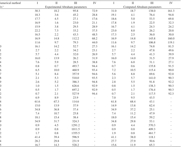
Table S5. The mean percentage deviation (MPD) of various numerical analyses employing the experimental and computed Abraham parameters of the

solutes and the overall (± SD) of MPDs

Numerical method No.a

I II III IV I II III IV

Experimental Abraham parameters Computed Abraham parameters

1 30.3 18.2 95.8 72.9 31.0 18.7 138.0 161.3

2 18.3 3.6 45.2 28.8 19.1 4.1 76.4 94.8

3 17.7 4.5 27.1 17.6 18.6 5.0 53.5 69.8

4 16.9 1.6 23.0 21.1 17.8 1.9 22.5 32.3

5 15.9 3.8 29.5 28.9 16.7 4.1 24.3 24.2

6 22.2 7.3 33.2 37.5 23.0 8.0 26.2 20.8

7 16.5 2.2 43.3 48.5 17.3 2.5 36.0 30.0

8 16.9 14.8 112.2 68.2 16.9 14.8 145.8 160.0

9 11.6 9.7 79.3 44.0 11.6 9.7 106.8 119.1

10 16.1 14.2 52.7 27.3 16.1 14.2 74.8 81.5

11 2.7 2.2 34.2 23.1 2.7 2.2 47.8 49.6

12 5.7 4.4 32.0 26.9 5.7 4.4 41.3 39.9

13 16.0 13.9 26.2 31.9 16.0 14.0 31.5 27.9

14 7.6 5.9 28.5 38.8 7.6 6.0 31.1 27.1

15 0.8 0.7 493.7 94.4 0.7 0.6 135.8 91.5

16 6.5 10.0 460.9 93.4 7.2 10.5 115.4 90.0

17 5.1 8.4 357.9 94.6 5.6 8.8 69.6 92.0

18 2.1 5.3 510.0 93.5 2.3 5.7 141.0 90.3

19 2.6 5.2 386.3 94.8 2.8 5.5 91.8 92.2

20 1.0 1.5 626.6 92.9 0.8 1.5 138.3 90.3

21 0.5 1.7 697.2 92.9 0.5 1.7 176.4 90.3

22 0.7 2.1 527.9 94.4 0.7 2.1 117.5 92.3

23 6.9 8.9 23.9 - 7.0 9.5 43.5

-24 61.6 67.3 114.6 - 61.8 68.4 43.1

-25 15.0 13.9 37.9 - 14.9 13.8 62.4

-26 34.8 36.8 37.4 - 34.9 37.2 25.1

-27 7.4 10.7 25.8 - 7.4 11.2 47.9

-28 18.1 15.4 38.4 - 18.0 15.4 59.2

-29 34.9 31.7 324.3 - 34.8 29.8 53.1

-30 0.9 4.5 1291.2 - 0.9 4.4 370.3

-31 0.9 0.8 1011.5 - 0.9 0.8 409.3

-32 1.7 0.8 1355.5 - 1.9 0.8 461.7

-33 41.4 39.4 596.9 - 41.1 38.0 118.1

-34 28.2 29.8 231.9 - 27.7 27.9 50.6

(14)

-Jouybanet al. S7 Vol. 19, No. 3, 2008

Numerical method No.a

I II III IV I II III IV

Experimental Abraham parameters Computed Abraham parameters

36 35.5 34.5 348.6 - 34.4 32.9 61.1

-37 36.2 37.2 282.8 - 32.2 35.8 87.7

-38 35.6 36.6 268.2 - 31.0 35.0 87.3

-39 28.2 29.8 231.9 - 27.7 27.9 50.6

-40 35.5 34.5 349.0 - 34.3 32.8 61.2

-41 32.2 28.3 581.9 - 32.3 26.4 83.7

-42 32.2 28.3 581.9 - 32.3 26.4 83.7

-43 2.2 0.6 1208.1 - 5.3 0.6 602.1

-44 1.3 3.3 1811.2 - 1.1 3.3 547.9

-45 2.4 3.5 23.1 16.3 2.6 3.7 21.3 30.7

46 4.7 3.5 26.5 31.5 4.3 3.1 28.6 22.7

47 1.9 4.1 26.8 12.8 2.2 4.6 29.5 26.8

48 5.4 4.2 36.7 27.6 5.0 3.8 38.0 18.2

49 1.1 1.3 11.2 3.6 1.1 1.4 4.7 48.6

50 1.9 0.7 32.4 39.1 2.0 0.5 39.3 11.2

51 6.0 8.4 30.3 17.5 6.0 8.5 36.9 18.4

52 2.0 1.1 42.0 33.2 2.0 1.4 47.7 5.6

53 1.1 0.3 37.6 41.7 1.1 0.3 46.5 15.1

54 6.4 6.2 28.3 25.7 6.4 6.2 37.4 11.0

55 4.7 2.6 36.7 25.6 4.7 2.7 44.7 7.5

56 2.1 3.4 18.7 12.3 2.1 3.6 17.9 34.2

57 5.1 3.3 22.3 27.5 4.7 3.0 25.0 23.5

58 2.1 3.6 23.1 9.9 2.3 4.0 26.4 29.2

59 5.2 5.1 32.7 24.7 4.8 4.7 34.7 18.2

60 0.2 1.1 45.5 - .2 1.1 88.3

-61 10.0 12.7 42.0 - 9.5 12.5 96.1

-62 17.2 17.0 52.5 - 16.6 16.7 51.4

-63 3.3 0.3 28.9 - 3.1 0.3 160.3

-64 1.0 0.2 27.7 - .9 0.2 167.5

-65 1.1 0.7 - - 1.1 0.7 -

-66 1.1 0.5 - - 1.0 0.5 -

-67 0.9 2.6 - - 1.0 2.6 -

-68 0.5 2.3 - - 0.5 2.3 -

-69 36.0 33.4 70.1 40.3 35.9 33.3 54.8 35.2

70 31.2 28.3 77.3 49.9 31.1 28.1 65.8 39.0

71 26.5 23.3 84.5 66.9 26.4 23.1 76.7 59.8

72 20.3 16.7 86.1 70.8 20.2 16.4 79.1 64.4

73 42.2 43.0 61.7 55.2 42.1 42.9 52.4 53.0

74 45.1 45.8 71.3 56.0 44.9 45.7 59.6 50.4

75 43.3 44.1 77.1 58.2 43.1 43.9 67.4 53.1

76 40.5 41.4 80.3 61.9 40.3 41.2 71.8 54.0

77 11.4 16.5 274.9 98.3 10.4 16.8 994.3 97.9

78 6.4 6.6 158.9 99.0 6.9 6.5 620.2 98.8

79 6.1 9.3 263.2 98.4 6.2 9.5 901.2 97.9

80 14.7 19.3 323.8 98.3 13.4 19.5 1096.2 97.9

81 2.1 4.0 439.8 97.9 2.1 4.0 1823.2 97.4

82 3.7 3.0 458.7 97.8 3.6 3.0 1769.7 97.3

83 8.1 11.3 58.9 80.5 8.1 10.4 55.9 166.5

84 6.7 4.8 60.1 50.1 7.0 5.0 46.7 70.7

85 16.8 12.5 66.0 49.1 17.3 13.1 51.7 40.8

86 8.6 7.1 78.3 48.0 8.8 7.3 61.9 25.0

87 6.7 6.8 50.0 101.5 6.5 7.4 70.9 197.5

88 11.0 9.6 43.9 65.1 10.2 9.0 43.7 119.7

89 7.9 8.1 54.0 48.4 7.9 8.3 40.5 59.6

90 4.7 5.3 74.9 48.9 4.9 5.8 58.3 34.4

Overall: 13.7 12.7 228.7 53.5 13.6 12.5 168.9 62.7

SD 14.0 13.9 337.7 30.0 13.8 13.7 325.4 43.6

a_{Details of the data is the same as Table S1.}

(15)

S8

Table S6. The individual percentage deviations (IPDs) of solubilities of solutes in some of the solvents of this work predicted by equations (1) and (2)

employing experimental and computed Abraham parameters

Solute Solvent T(nC) Experimental parameters Computed parameters

equation (1) equation (2) equation (1) equation (2)

Benzoic acid Carbon tetrachloride 25 336.2 95.2 100.8 92.1

Benzoic acid Carbon tetrachloride 30 258.9 96.1 65.2 93.5

Benzoic acid Cyclohexane 25 690.6 93.4 176.6 90.9

Benzoic acid Cyclohexane 30 522.7 94.8 117.8 92.9

Benzoic acid Heptane 25 569.9 92.1 101.2 89.3

Benzoic acid Heptane 30 419.5 93.9 56.0 91.7

Benzoic acid Hexane 25 708.0 92.1 177.1 89.2

Benzoic acid Hexane 30 541.2 93.7 119.9 91.5

Benzophenone Carbon tetrachloride 25 49.2 - 64.4

-Benzophenone Decane 25 28.7 - 25.9

-Benzophenone Dodecane 25 182.0 - 64.7

-Benzophenone Heptane 25 7.6 - 51.1

-Benzophenone Hexane 25 87.7 - 8.3

-Benzophenone Nonane 25 15.4 - 33.2

-Benzophenone Octane 25 15.7 - 32.3

-Carbazole 2,2,4-Trimethylpentane 25 761.8 - 158.0

-Carbazole Cyclohexane 25 1967.8 - 661.6

-Carbazole Dibutyl ether 25 391.4 - 57.4

-Carbazole Heptane 25 333.7 - 193.8

-Carbazole Hexadecane 25 1017.3 - 280.2

-Carbazole Hexane 25 835.7 - 282.4

-Carbazole Methyl cyclohexane 25 557.4 - 470.5

-Carbazole Heptane 25 333.7 - 193.8

-Carbazole Hexane 25 835.7 - 282.4

(16)

-Jouybanet al. S9 Vol. 19, No. 3, 2008

Solute Solvent T(nC) Experimental parameters Computed parameters

equation (1) equation (2) equation (1) equation (2)

Naphthalene Benzene 25 16.5 8.7 9.4 43.0

Naphthalene Carbon tetrachloride 25 33.6 29.8 37.1 8.7

Naphthalene Cyclohexane 25 28.7 46.1 39.0 21.6

Naphthalene Hexadecane 25 34.7 20.5 42.4 9.3

Naphthalene Hexane 25 46.6 37.3 54.1 8.7

Naphthalene Toluene 25 6.6 0.4 0.9 51.1

p-Benzoquinone 2,2,4-Trimethylpentane 25 54.8 - 44.4

-p-Benzoquinone Carbon tetrachloride 25 68.0 - 8.8

-p-Benzoquinone Cyclohexane 25 37.6 - 126.9

-p-Benzoquinone Dodecane 25 47.5 - 83.3

-p-Benzoquinone Heptane 25 16.7 - 215.2

-p-Benzoquinone Octane 25 45.7 - 89.6

-Phenanthrene 2,2,4-Trimethylpentane 20 46.7 41.8 17.6 72.5

Phenanthrene 2,2,4-Trimethylpentane 30 71.9 25.2 56.5 9.0

Phenanthrene Heptane 20 20.5 173.4 64.2 228.3

Phenanthrene Toluene 20 59.1 29.2 39.7 14.2

Phenyl acetic acid 2,2,4-Trimethylpentane 25 561.6 97.1 2363.6 96.5

Phenyl acetic acid Carbon tetrachloride 25 76.9 99.3 283.1 99.0

Phenyl acetic acid Cyclohexane 25 339.2 98.6 1405.1 98.2

Phenyl acetic acid Heptane 25 574.0 96.9 2107.4 96.2

Phenyl acetic acid Octane 25 701.5 97.2 2677.3 96.6

Pyrene Heptane 20 67.2 8.8 19.2 82.6

Pyrene Heptane 30 75.7 32.5 40.2 35.2

Pyrene Heptane 40 85.8 60.6 65.1 21.1

Pyrene Heptane 50 92.5 79.0 81.4 57.9

Pyrene Toluene 20 105.4 284.4 188.8 394.2

Pyrene Toluene 30 30.2 143.6 83.0 213.2

Pyrene Toluene 40 6.4 99.2 49.6 156.1

Pyrene Toluene 50 43.8 5.2 21.0 35.2

All 207.2a _59.1b _188.0a _73.6b

25 343.6c _62.6d _331.1c _76.2d

a_{The difference was not statistically significant (paired t-test, p>0.05);}b_{The difference was statistically significant (paired t-test, p<0.008);}c_The

differ-ence was not statistically significant (paired t-test, p>0.05); d_{The difference was not statistically significant (paired t-test, p>0.05).}