Brazilian Journal of Physics, vol. 34, no. 1A, March, 2004 307
Spinodal Instability in the Quark-Gluon Plasma
C. E. Aguiar, E. S. Fraga, and T. Kodama
Instituto de F´ısica, Universidade Federal do Rio de JaneiroC.P. 68528, Rio de Janeiro, 21941-972, RJ, Brazil
Received on 15 August, 2003.
We investigate the onset of spinodal decomposition in a relativistic fluid of quarks coupled to a nonequilibrium chiral condensate. Studying small fluctuations around equilibrium, we identify the role played by sound and chiral waves in the generation of unstable modes.
The hadronization of the quark-gluon plasma (QGP) possibly produced in the early universe or in high-energy heavy-ion collisions may proceed in a number of differ-ent ways, depending on the nature of the QCD phase tran-sition. In the heavy-ion case, some results from CERN-SPS and BNL-RHIC suggest what has been calledsudden hadronization [1] or explosive behavior [2, 3]. From the theoretical side, this phenomenon has been associated as-sociated with deep supercooling of the QGP followed by spinodal decomposition, and also to rapid changes in the ef-fective potential of QCD near the critical temperature, such as predicted, for instance, by the Polyakov loop model [4]. Clearly, an understanding of the interplay between the typi-cal space and time stypi-cales of the expanding plasma is wel-come. Some attempts in this direction can be found in Refs. [5, 6, 7, 8, 9, 10, 11, 12, 13].
In this paper, we discuss the onset of spinodal instability in an expanding plasma. As a phenomenological model to mimic the case of the QGP, we use a relativistic plasma of quarks coupled to a chiral field. The later is not necessarily in thermal equilibrium with the quark fluid. Although we derive a phenomenologicalnonequilibrium chiral hydrody-namicsfrom a variational principle, we do not focus on the numerical solution of the resulting hydrodynamic transport equations.
To model the mechanism of chiral symmetry breaking present in QCD, we adopt a simple low-energy effective chi-ral model: the linearσ-model coupled to quarks [14], which in turn comprise the hydrodynamic degrees of freedom of the system. Similar approaches, relying on low-energy ef-fective models for QCD and making use of a number of tech-niques to treat the expanding plasma, can be found in the lit-erature [5, 6, 7, 8, 9]. The gas of quarks provides a thermal bath in which the long-wavelength modes of the chiral field evolve. The latter plays the role of an order parameter in a Landau-Ginzburg description of the chiral phase transition [8, 9].
Let us consider a chiral fieldφ = (σ, ~π), whereσis a scalar field andπiare pseudoscalar fields playing the role of
the pions, coupled to two flavors of quarks according to the
Lagrangian:
L=q[iγµ∂µ+µqγ0−W(φ)]q+ 1 2∂µφ∂
µφ−V(φ). (1)
Hereq= (u, d)is the constituent-quark field andµq =µ/3
is the quark chemical potential. The interaction between the quarks and the chiral field is given byW(φ) = g(σ+
iγ5~τ ·~π), andV(φ) = (λ2/4)(σ2+~π2−v2)2−hqσ is
the self-interaction potential forφ. The parameters above are chosen such that chiralSUL(2)⊗SUR(2)symmetry is
spontaneously broken in the vacuum. The vacuum expecta-tion values of the condensates arehσi = fπ andh~πi = 0,
wherefπ = 93 MeV is the pion decay constant. The
ex-plicit symmetry breaking term is due to the finite current-quark masses and is determined by the PCAC relation, giv-inghq = fπm2π, wheremπ = 138MeV is the pion mass.
This yieldsv2 =f2
π−m2π/λ2. The value ofλ2= 20leads
to aσ-mass,m2
σ = 2λ2fπ2+m2π, equal to 600 MeV. The
quark-chiral field coupling constant is taken to beg = 3.3, for which the constituent quark mass is307MeV, about 1/3 of the nucleon mass.
In what follows, we treat the gas of quarks as a heat bath for the chiral field, with temperatureTand baryon-chemical potentialµ. Integrating over the fermionic degrees of free-dom and using a classical approximation for the chiral field, we can write the thermodynamic potential as
Ω(T, µ, φ) =V(φ)−T
V ln det{[G −1
E +W(φ)]/T}, (2)
whereGE is the fermionic Euclidean propagator andV is
the (infinite) volume of the system. The determinant that results from the functional integration over the quark and anti-quark fields can be calculated to one-loop order in the standard fashion [15, 16]. As already mentioned, the chiral fieldφplays the role of an order parameter, its equilibrium value corresponding to the minimum of the grand canonical potential (2) for given(T, µ).
308 C.E. Aguiar, E.S. Fraga, and T. Kodama
dynamics. This approach provides a natural way of merging chiral and fluid dynamics in a unified Lagrangian system. For a different treatment of the hydrodynamics of nuclear matter in the chiral limit, see [18].
We describe the state of the fluid in terms of the four-velocityuµ(x) = (γ, γ~v), where~v(~r, t)is the flow velocity
of matter, the proper baryon density, n(x), and the proper entropy density, s(x). The action of the fluid-chiral field system is then defined as
S ≡ Z
d4x
·1
2∂µφ∂
µφ−ǫ(n, s, φ) ¸
, (3)
whereǫ= Ω +T s+µnis the energy density, from which the temperature and chemical potential are obtained by the usual thermodynamic relations: T = ∂ǫ(n, s, φ)/∂s and
µ = ∂ǫ(n, s, φ)/∂n. The variation of n,s anduµ in the
action principle is performed under constraints arising from baryon number conservation,∂µ(nuµ) = 0, entropy
conser-vation, ∂µ(suµ) = 0, and normalization of the 4-velocity,
uµu
µ = 1. With these conditions the variational principle,
δS = 0, leads to the equations of motion:
✷φ=−R , (4)
uµ∂µ(wuν) =−(∂µuµ)wuν+∂νp+R∂νφ , (5)
wherep=−Ωis the pressure,w=ǫ+p=T s+µnis the enthalpy density, and
R=∂Ω(T, µ, φ)/∂φ=∂ǫ(n, s, φ)/∂φ (6) gives the dynamical coupling between the fluid and the chi-ral field. Note thatRhas four components, and can be writ-ten as
R= ∂V(φ)
∂φ +gρ(T, µ, φ), (7)
where the (scalar/pseudoscalar) densityρis
ρ=gφνq
Z d3k
(2π)3
1/Ek(φ)
e[Ek(φ)−µq]/T+ 1 + (µq → −µq).
(8) Hereνq = 12stands for the color-spin-isospin degeneracy
of the quarks, Ek(φ) = (~k2+m2q(φ))1/2, and mq(φ) = (g2φ2)1/2 = g(σ2+~π2)1/2 plays the role of an effective
mass for the quarks.
Equation (5) is the relativistic Euler equation for the quark fluid in the presence of the chiral field. Introducing the energy-momentum tensor of the fluid in the usual way,
Tµν =wuµuν−pgµν, we can write the Euler equation as
∂µTµν =R∂νφ . (9)
The total energy-momentum tensor of the fluid-field sys-tem,Tµν =Tµν−1
2∂αφ∂
αφgµν+∂µφ∂νφ, is, of course,
conserved. Different derivations and equivalent forms of Eqs. (4)–(9) can be found in [5, 6, 9].
Numerical studies of the system above have been done extensively in Refs. [6, 9]. Here, we refrain from this ap-proach and, instead, analyze the behavior of small perturba-tions around equilibrium. We writeψ(x) =ψeq+ψ1e−iKx,
whereψstands forn,s,~vorφ, andKµ= (ω, ~k).ψ eq
cor-responds to a situation of stable or metastable equilibrium, given by the equation R = 0. Keeping terms up to first order in the perturbationψ1, the field and hydrodynamical
equations become
(ω2−~k2−m2π)~π1 = 0, (10)
(ω2−~k2−m2σ)σ1 =
k ωweqR
′v
1, (11)
(ω2−p′~k2)v
1 = ωkR′σ1, (12)
where the masses of the σ and ~π fields are m2
σ =
(∂2ǫ(n, s, φ)/∂σ2)
eqandm2π = (∂2ǫ(n, s, φ)/∂π2)eq. We
have also definedp′ ≡ [∂p/∂ǫ]
eq andR′ ≡ [∂Rσ/∂ǫ]eq,
evaluated at constant(s/n)andφ. The flow velocity~v1 is
parallel to the wave vector~k (sound waves are longitudi-nal), and its magnitude determines the baryon number and entropy amplitudes:
n1= (k/ω)neqv1, (13)
s1= (k/ω)seqv1. (14)
We see from the linearized equations (10)–(12) that, to first order, only theσfield is coupled to the hydrodynamic degrees of freedom. The dispersion relation for the coupled modes reads
(ω2−p′~k2)(ω2−~k2−m2
σ) =weqR′
2~k2.
(15)
For long wavelength fluctuations we can approximate the roots of (15) by
ω2
s/~k2 = p′−
M2
m2
σ
+O(~k2), (16)
ω2σ = m2σ+O(~k2), (17)
whereM2 ≡ w
eqR′2. These modes can be identified as
sound waves (frequency ωs) and chiral waves (frequency
ωσ).
The onset of instabilities takes place whenω2 <0,i.e., either for(p′−M2/m2
σ)<0or form2σ<0. From Eq. (16),
however, we see that sound waves become unstable before chiral waves do.
Let us now discuss the onset of this spinodal instabil-ity in different portions of the phase diagram of the linear
Brazilian Journal of Physics, vol. 34, no. 1A, March, 2004 309
5 0 0 6 0 0 7 0 0 8 0 0 9 0 0 1 0 0 0
ch e m ica l p o te n tia l (M e V )
04 0 8 0 1 2 0
te
m
p
e
ra
tu
re
(
M
e
V
)
coe xiste n ce spin o d a l E
Figure 1. Phase diagram for the effective model in the(µ, T) -plane. The coexistence curve ending at the critical pointEis rep-resented by the solid line. The spinodal curves are shown as dashed lines.
In Fig. 1 we plot the phase diagram in the(µ, T)-plane. The coexistence curve is represented by the solid line. It ends at a critical point, E, located atTE = 98MeV and
µE = 630 MeV. The spinodal lines (p′ −M2/m2σ = 0)
corresponding to supercooling and superheating are shown as dashed lines.
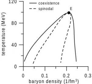
A more illuminating picture of the unstable region is given by the phase diagram in the(n, T)-plane, as shown in Fig. 2. As before, the phase coexisting border is represented by the solid line and dashed lines stand for the spinodals. The sector on the right of the critical pointE corresponds to supercooled states in the chirally symmetric phase. The domain inside the dashed lines corresponds to the spinodal unstable states.
0
0 .1
0 .2
0 .3
b a ryo n d e n sity (1 /fm
3)
0
4 0
8 0
1 2 0
te
m
p
e
ra
tu
re
(
M
e
V
)
coe xiste nce spin o da l E
Figure 2. Phase diagram for the effective model in the(n, T) -plane. Line conventions are the same as in Fig. 1.
To summarize, we have shown that spinodal decompo-sition in the QGP proceeds by the exponential increase of hydrodynamical sound-like modes. We have mapped the
boundaries of the unstable region, determining how much supercooling (or superheating) is necessary to trigger spin-odal instability. In the case of relativistic heavy ion reac-tions, the rapid time scale of expansion and effects due to the finite size of the system could change significantly these results. In order to investigate these effects in a realistic and quantitative way, one should perform numerical simulations of the evolution of the instability in different scenarios. In particular, one should study the limits of the linear approx-imation at large times. Results in this direction will be pre-sented elsewhere.
Acknowledgments This work was partially supported by CAPES, CNPq, FAPERJ and FUJB/UFRJ.
References
[1] J. Rafelski and J. Letessier, Phys. Rev. Lett.85, 4695 (2000).
[2] A. Dumitru and R. D. Pisarski, Nucl. Phys. A 698, 444 (2002).
[3] O. Scavenius, A. Dumitru and A. D. Jackson, Phys. Rev. Lett. 87, 182302 (2001).
[4] R. D. Pisarski, Phys. Rev. D62, 111501 (2000); A. Dumitru and R. D. Pisarski, Phys. Lett. B504, 282 (2001).
[5] L. P. Csernai and I. N. Mishustin, Phys. Rev. Lett.74, 5005 (1995); A. Abada and J. Aichelin, Phys. Rev. Lett.74, 3130 (1995); A. Abada and M. C. Birse, Phys. Rev. D55, 6887 (1997).
[6] I. N. Mishustin and O. Scavenius, Phys. Rev. Lett.83, 3134 (1999).
[7] O. Scavenius and A. Dumitru, Phys. Rev. Lett. 83, 4697 (1999).
[8] O. Scavenius, A. Dumitru, E. S. Fraga, J. T. Lenaghan and A. D. Jackson, Phys. Rev. D63, 116003 (2001).
[9] K. Paech, H. St¨ocker and A. Dumitru, nucl-th/0302013.
[10] E. E. Zabrodin, L. V. Bravina, L. P. Csernai, H. St ¨ocker and W. Greiner, Phys. Lett. B423, 373 (1998).
[11] P. Shukla and A. K. Mohanty, Phys. Rev. C 64, 054910 (2001).
[12] C. Spieles, H. St¨ocker and C. Greiner, Phys. Rev. C57, 908 (1998).
[13] E. S. Fraga and R. Venugopalan, arXiv:hep-ph/0304094.
[14] M. Gell-Mann and M. Levy, Nuovo Cim.16, 705 (1960); R. D. Pisarski, Phys. Rev. Lett.76, 3084 (1996).
[15] O. Scavenius, A. Mocsy, I. N. Mishustin and D. H. Rischke, Phys. Rev. C64, 045202 (2001).
[16] J. Kapusta, Finite Temperature Field Theory (Cambridge University Press, Cambridge, 1989).
[17] H. T. Elze, Y. Hama, T. Kodama, M. Makler and J. Rafelski, J. Phys. G25, 1935 (1999).