Energy averages and fluctuations in the decay out of superdeformed bands

Energy averages and fluctuations in the decay out of superdeformed bands

A. J. Sargeant,1M. S. Hussein,1M. P. Pato,1and M. Ueda2

1_{Nuclear Theory and Elementary Particle Phenomenology Group, Instituto de Fı´sica, Universidade de Sa˜o Paulo,} Caixa Postal 66318, 05315-970 Sa˜o Paulo, Brazil

2_{Institute of Physics, University of Tsukuba, Ten-noudai 1-1-1, Tsukuba, Ibaraki, 305-8571, Japan}

~Received 20 March 2002; published 4 December 2002!

We derive analytic formulas for the energy average~including the energy average of the fluctuation contri-bution!and variance of the intraband decay intensity of a superdeformed band. Our results may be expressed in terms of three dimensionless variables:G↓_/G

S, GN/d, and GN/(GS1G↓). HereG↓is the spreading width for the mixing of a superdeformed~SD!stateu0&with the normally deformed~ND!statesuQ&whose spin is the same asu0&’s. TheuQ&have mean lever spacingdand mean electromagnetic decay widthGNwhilstu0&has electromagnetic decay widthGS. The average decay intensity may be expressed solely in terms of the variables

G↓

/GSandGN/dor, analogously to statistical nuclear reaction theory, in terms of the transmission coefficients T₀(E) andTN describing transmission from the uQ& to the SD band via u0& and to lower ND states. The variance of the decay intensity, in analogy with Ericson’s theory of cross section fluctuations, depends on an additional variable, the correlation lengthGN/(GS1G↓)5(d/2p)TN/(GS1G↓). This suggests that analysis of an experimentally determined variance could yield the mean level spacingd as does analysis of the cross section autocorrelation function in compound nucleus reactions. We compare our results with those of Gu and Weidenmu¨ller.

DOI: 10.1103/PhysRevC.66.064301 PACS number~s!: 21.60.2n, 24.60.2k

I. INTRODUCTION

The basic feature to be explained in the decay out of superdeformed~SD!rotational bands@1– 4#is that the inten-sity of the collectiveg rays emitted during the cascade down an SD band remains constant until a certain spin is reached whereafter it drops to zero within a few transitions. The sharp drop in intensity is believed to arise from mixing of the SD states with normally deformed ~ND! states of identical spin@5#. The model of Refs.@6 –9#attributes the suddenness of the decay out to the spin dependence of the barrier sepa-rating the SD and ND minima of the deformation potential. References@10–12#discuss the effect of the chaoticity of the ND states on the decay out.

In the present paper, we derive analytic formulas for the energy average~including the energy average of the fluctua-tion contribufluctua-tion!and variance of the intraband decay inten-sity of a superdeformed band in terms of variables which usefully describe the decay out @3,4,13,14#. We achieve this using the MIT approach to statistical nuclear reaction theory @15–17#. The MIT approach tackles calculation of the fluc-tuation cross section and other moments of theS matrix by directly calculating averages of fluctuating functions of en-ergy.

In agreement with Gu and Weidenmu¨ller @13# ~GW! we find that average of the total intraband decay intensity can be written as a function of the dimensionless variables G↓_/G

S

andGN/d, whereG↓is the spreading width for the mixing of

an SD state with normally ND states of the same spin, d is the mean level spacing of the latter and GS (GN) are the

electromagnetic decay widths of the SD ~ND! states. Our formula for the variance of the total intraband decay inten-sity, in addition to the two dimensionless variables just men-tioned, depends on the dimensionless variable GN/(GS

1G↓_{). This additional variable is analogous to the}

correla-tion width of the Ericson’s theory of cross seccorrela-tion fluctua-tions. Its appearance suggests that measurement of the vari-ance of the decay intensity could yield the mean level spacingd.

The paper is organized in the following manner. In Sec. II we express the average decay intensity as an average term plus the average of a fluctuation term. In Sec. III the expres-sion for the average decay intensity obtained in Sec. II is evaluated approximately. In Sec. IV we calculate the vari-ance of the intensity within the same approximation scheme as Sec. III. In Sec. V we interpret our results by analogy with statistical nuclear reaction theory, expressing our results in terms of transmission coefficients and compare our results with those of GW. In particular we suggest a reason why GW did not observe the variable G_N/(G_S1G↓

) in their calcula-tion of the variance. Finally in Sec. VI we make some con-cluding remarks incon-cluding mention of the limitations of our results.

II. ENERGY AVERAGES AND FLUCTUATIONS

The total intraband decay intensity has the form @12,13,18#

I_in5~2pGS!21

E

2`

`

dEuA₀₀~E!u2_{, ~1!}

where the intraband decay amplitude is given by

A₀₀~E!₅gS

^

˜0uG~E!u0

&

gS. ~2!

Here gS is the electromagnetic decay amplitude of

superde-formed stateu0

&

defined such thatGS5gS

2_{. We assume that} the amplitude feeding u0

&

is also given by gS. The total

G~E!₅~E₂H!21_{, ~3!} where the full nuclear Hamiltonian is denoted byHand has a non-Hermitian part which accounts for coupling to the electromagnetic field @see Eqs. ~5!, ~18!, and ~19! below#. The tilde is used to indicate the dual state or adjoint@15#of u0

&

.

In what follows we employ the optical background repre-sentation introduced Kawai, Kerman, and McVoy @16#. These authors investigated fluctuation cross sections using a representation of the S matrix in which the background S matrix is chosen to be the energy average of the S matrix itself, that is, the S matrix corresponding to the optical po-tential. Here we use the same idea to decompose the decay amplitude, Eq. ~2!, into the sum of its Lorentzian energy average~Lorentzian energy averaging intervalI),

A₀₀~E![A₀₀~E₁iI/2!, ~4!

plus a fluctuating part.

We proceed by introducing Feshbach’s projection opera-tors @15#

P₅u0˜

_&^

_{0u and Q512P. ~5!}

Let us introduce the notation G₅PG P for the effective Green’s function in the P space and let H_{P P5}PH P, H_PQ

5PHQ, etc. Using the techniques of Ref.@16#we obtain

G₅G¯₁Gfl, ~6! where the average effective Green’s function ¯G₅G(E

1iI/2) is given by

G

¯_5@E2H¯_#21 _~7!

and the average effective Hamiltonian is given by

H¯₅HP P1W¯P P, ~8!

where coupling to the eliminatedQspace is accounted for by

W¯P P5HPQ

1

E₂H_QQ1iI/2HQ P5

22i

I VPQVQ P ~9!

and the energy dependent coupling potentialVintroduced in Ref. @16#is defined by

VPQ5HPQ

A

iI/2 E2HQQ1iI/2

,

VQ P5

A

iI/2

E₂H_QQ1iI/2HQ P.

The fluctuating part of the effective Green’s function G is given by

Gfl₅G¯ VPQ

1

E₂H_QQ2W_QQVQ PG¯, ~10!

where coupling back to the Pspace is accounted for by

W_QQ5V_{Q P}¯ VG _PQ. ~11!

By construction Gfl₅0 in so much as ¯G is unchanged by reaveraging, that is ifG¯¯₅G¯.

The corresponding decomposition of Eq. ~2!for the tran-sition amplitude is

A₀₀~E!5A₀₀~E!1A₀₀fl~E!, ~12! where the energy average of the transition amplitude is

A005gSG¯00gS ~13!

and the fluctuating part of the transition amplitude is

A₀₀fl₅gSG00 fl_g

S. ~14!

Thus the average of Eq.~1!for the relative intensity may be written as the incoherent sum

I_in ¯_5I

in av

1I_infl, ~15! where

I_inav₅I_inav₅~2pG_S!21

E

2` `

dEuA₀₀~E!u2 _~16!

and

I_infl₅~2pGS!21

E

2`

`

dEuA₀₀fl~E!u2_{. ~17!}

Up to this point no assumptions have been made except that the transition amplitude can be written in the form of Eq.~2!. As will be made clear in Sec. III the meaning of this assump-tion is thatu0

&

is a doorway for the decay from the SD band to the ND states and vice versa. In the manipulations subse-quent to Eq.~2!we have put the average intensity in a form consisting of a background term coming from the smooth energy dependence of the doorway plus a term resulting from fluctuations on this background.

The representation we have used is particularly suitable for approximation when the ND states are overlapping. In Sec. III we evaluate Eqs. ~15!–~17! for the average decay intensity I_in assuming that this is the case. In Sec. IV we calculate the variance which describes the way in whichIin fluctuates aboutIin.

III. AVERAGE DECAY INTENSITY

Let us assume thatHP P satisfies the eigenvalue equation

HP Pu0

&

5~E02iGS/2!u0

&

~18!

andHQQ

Here,E0 denotes the energy of SD stateu0

&

, GS it’s

electro-magnetic width for decay to the next lowest state in the SD band,EQ (Q51, . . . ,N) the energy of theNND statesuQ

&

with the same spin asu0

&

andGN the common

electromag-netic width of theuQ

&

for decay to ND states of lower spin. Further, let us write the matrix element ofWP P, Eq.~9!,

as

W¯₀₀₅

^

0uW¯_{P P}u0

&

5D↓ 2iG↓

/2. ~20!

Here, D↓

5ReW¯₀₀ is an energy shift that we ignore and G↓ 522 ImW¯₀₀. Combining these definitions with Eqs. ~7!, ~8!, and~13!the average of the transition amplitude can be written as

A₀₀₅ GS

E₂E₀₁i~ GS1G↓!/2

. ~21!

We see that Eq. ~21! exhibits the structure of an isolated doorway resonance. The doorway u0

&

has an escape width GS for decay to the SD state with next lower spin and a

spreading widthG↓ _{for decay to the ND states with the same}

spin which are reached by tunneling through the barrier sepa-rating the SD and ND wells. The doorway structure of Eq. ~21! is due to the assumption that the transition amplitude can be written as in Eq.~2!. The most general expression for the transition amplitude has the form A_ab5gab

1(cc₈gac

^

cuGuc

8

&

gc₈b, where gac describes the coupling

of channelsaandc. In our doorway model thecandc

₈

stand for u0

&

or uQ

&

, Q₅1, . . . ,N, i.e., (cuc

&^

cu5P1Q, and a

and b denote channels the ~electromagnetic! coupling to which is taken is accounted for by the non-Hermitian part of H@Eqs.~18!and~19!#, that is they denote the SD state above u0

&

, the SD belowu0

&

, and ND states whose spin is different from that of u0

&

. The direct coupling of channelsa andb, gab, is taken to be zero.

In order to evaluateA₀₀fl it is useful to introduce eigenvec-tors and eigenvalues of the operator HQQ1WQQ defined by

~HQQ1WQQ!uq

&

5~Eq2iGq/2!uq

&

, q51, . . . ,N.

~22!

Then from Eq. ~14!and Eq.~10!for Gflwe obtain

A₀₀fl₅gSG¯00

(

q

^

˜0uV_PQuq

&^

˜quV_{Q P}u0

&

E₂Eq1iGq/2

G ¯

00gS

5A₀₀

(

q

g0qgq0/GS

E₂E_q1iG_q/2A00, ~23!

where

g₀q5

^

˜0uVPQuq

&

, ~24!

gq05

^

˜quVQ Pu0

&

. ~25!

We now employ some statistical assumptions which are fre-quently used in statistical nuclear reaction theory@15#to de-rive an analytic formula for the decay intensityI_in. We shall assume that the Lorentzian and box energy averages and the average over the labelqare all approximately equal, i.e., that for a suitable function fq(E) ofq andE,

f_q~E!5f_q~E₁iI/2!' 1

DE

E

E₀1DE/2

E01DE/2

dE

₈

f_q~E

₈

!

'1

N q5

(

1

N

f_q~E!. ~26!

The width of the box average,DE, is related to the width the Lorentzian energy average by DE'pI/2 and to the mean spacingdof theNND states byDE'Nd. This approxima-tion is good as long as G/d_@1 @see Eq.~39! below for the definition of G]. Within these assumptions we see from Eq. ~9!that theg₀q andgq0 are related toW¯00 by

W¯005

22i

I

(

q

g0qgq0'

2pi DE

(

q

g0qgq0'

2pi d g0qgq0.

~27!

Thus the spreading with is given by

G↓

52_dpRe g₀qgq0 ~28!

and the energy shift by

D↓

5p_dIm g_0qg_q0. ~29!

From Eq.~23!we can calculate the amplitude autocorrelation function

A₀₀fl~E!A₀₀fl~E

₈

!*₅ 1

G_S2A00~E! 2

(

qq₈

g0qgq0g0*q₈gq*₈0

~E2Eq1iGq/2!~E

8

2Eq₈2iGq₈/2!

A₀₀~E

₈

!*2 _~30!

5 1

G_S2A00~ «

¯_1«/2!2

₍

qq₈

g_0qg_q0g_0q

8

* g_q

80

*

~ «¯1«/2₂Eq1iGq/2!~ «¯2«/22Eq₈2iGq₈/2!

where we have made the variable changes «₅E₂E

₈

and¯«_5(E1E

₈

_{)/2. Consider the middle factor in Eq. ~31!which we} anticipate is a function of« only

a~ « !5

(

qq₈

g₀qgq0g0*q₈gq*₈0 ~ «¯_{1«/22Eq1iGq/2!~ «}¯_2«/22Eq

82iGq₈/2!

. ~32!

We interpret the energy average in Eq. ~32!to be an average over¯«_{. Employing a box energy average}

a~ « !' 1 DE

(

_qq

8

E

E₀2DE/2

E₀1DE/2

d¯« g0qgq0g0q8

* g_q

80

*

~ «¯1«/22E_q1iG_q/2!~ «¯2«/22E_q82iG_q8/2!. ~33!

IfDE is large compared to theGq but small enough for the

EqandGq to be treated as constants then we may extend the

limits of integration to 6` and perform the integral using the calculus of residues to obtain

a~ « !'2pi DE

(

_qq

8

g0qgq0g0*q₈gq*₈0 «1Eq₈2Eq1i~ Gq₈1Gq!/2

. ~34!

Assuming that the phases of the g₀q and the gq0 are ran-domly distributed as a function of q the double sum in Eq. ~34!collapses to a single sum giving

a~ « !'2pi DE

(

q

ug₀qgq0u2 «₁iGq

. ~35!

Then employing the definition of the average given by Eq. ~26!

a~ « !'2pi

d

F

ug₀qgq0u2 «1iGq

G

. ~36!

Assuming that the average of a ratio is equal to the ratio of the averages we get

a~ « !'G

↓2 2p

id

«₁iG, ~37!

withG↓andGintroduced according to Eq.~38!and Eq.~39! below. The introduction of G↓ _{is based on the assumption}

that

ug₀qgq0u2'2ug0qgq0u2'2

F

G↓_d

2p

G

2

. ~38!

The factor of 2 which appears in the first manipulation in Eq. ~38! accounts for the self-correlation ~present since the en-trance and exit channel are both u0

&

) and is equal to the elastic enhancement factor for compound elastic scattering in the overlapping resonance region. In the second manipula-tion in Eq. ~38!we have again ignored the energy shift@see Eqs. ~28!and~29!#.

Equation~37!also introduces the correlation width

G'Gq ~39!

522 Im

^

˜quHQQ1WQQuq

&

~40!

5GN1G↑ ~41!

'GN, ~42!

where we used Eq.~19!for the electromagnetic width of the uQ

&

and introduced

G↑

522 Im

^

˜quWQQuq

&

522 Im

gq0g0q

E₂E₀₁i~ GS1G

↓

!/2

5G ↓_d

2p

~ GS1G↓!

~E₂E₀!2

1~ GS1G↓!2/4

,

~43!

which is the width for their decay back tou0

&

. The approxi-mations represented by Eqs. ~39!and~42!will be discussed in Sec. V. Using Eq.~37!and approximation~42!we finally obtain

A₀₀fl~E!A₀₀fl~E

₈

!*'2~2pG_N/d!21_{~ G}↓

/G_S!2A₀₀~E!2

3 iGN

E₂E

₈

₁iGN

A₀₀~E

₈

!*2_{. ~44!} WhenE

₈

₅E this reduces to

uA₀₀flu2

52~2pG_N/d!21 GS 2_G↓2

@~E₂E₀!21~ GS1G↓!2/4#2

, ~45!

which is the average of the fluctuation contribution to the transition intensity.

The integrals in Eqs. ~16! and ~17! for the average and fluctuation contributions to the total decay intensity may now be carried out using the calculus of residues. Substituting Eq. ~21!into Eq.~16!we obtain

I_inav₅ 1 11G↓_/G

S

Equation ~46! is identical with the equivalent result in GW ~see also Ref. @14#!. Substituting Eq. ~45!into Eq. ~17! we obtain

I_infl52~pGN/d!21

~ G↓/GS!2

~11G↓

/G_S!3 ~47!

52~pGN/d!21Iinav~12Iinav!2 ~48! for the average fluctuation contribution to the average decay intensity.

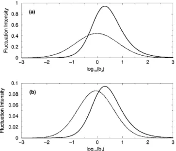
Equation~47!forI_infl is plotted in Fig. 1 and for compari-son we have also plotted a fit formula which was obtained by GW,

I_in[email protected]~ GN/d!0.2172#

3exp

H

₂

F

0.4343 ln

S

G

↓

GS

D

2

0.45

S

GN d

D

20.1303

G

2 ~ GN/d!20.1477

J

.

~49!

Qualitative agreement is seen between the two formulas. Note that Eq. ~49! yields a negative intensity for G_N/d

.1.51 which excludes its use in this regime. Our result which is only strictly valid when G_N/d_@1 is simply in-versely proportional toGN/d. The exact result of GW forIin fl @Eq. ~24! in GW# which can be used for any GN/d also

decreases monotonically with increasingGN/d.

The dependence of I_infl ~and that of I_inav) on G↓

/G_S results from the resonant doorway energy dependence of the decay amplitude A₀₀(E) @Eq. ~21!#. This energy dependence also manifests itself in the average of the fluctuation contribution

to the transition intensity uA₀₀fl(E)u2 _{@Eq. ~45!#. GW include} precisely the same energy dependence in their calculation by use of an energy dependent transmission coefficient to de-scribe decay to the SD band @see Eq. ~78! below and the discussion in Sec. V C#. This is the reason for our qualitative agreement with GW concerning Iin.

IV. VARIANCE OF THE DECAY INTENSITY

The error incurred in making the energy average is given by

DI_in5I_in2I_in5I_infl₂I_infl₁2 Re

E

2` `

dEA₀₀~E!A₀₀fl~E!*. ~50!

The average of the error vanishes:DI_in50. A measure of the dispersion of the calculatedI_inis given by the variance

~ DIin!25~Iin2Iin!2. ~51! In order to evaluate (DI_in)2 the averages indicated in Eq. ~51!must be performedbeforethe integration which appears in the definition ofI_in, Eq.~1!. We obtain

~ DI_in!2'~2pG_S!22

E

2` `

dE

E

2` `

dE

₈

$uA₀₀fl~E!A₀₀fl~E

₈

!*u2

12 ReA00~E!*A00fl~E!A00fl~E

8

!*A00~E

8

!%. ~52! In deriving Eq. ~52! we have used A₀₀fl(E)

5A₀₀fl(E)A₀₀fl(E

₈

)₅0, A₀₀fl(E)A₀₀fl(E

₈

)*Þ0 and A₀₀fl (E)A₀₀fl (E)*A₀₀fl (E

₈

)A₀₀fl (E

₈

)*5uA₀₀fl (E)u2 _uA

00 fl _(E

8

)u2

1uA₀₀fl(E)A₀₀fl(E

₈

)*u2 _{and we have assumed that averages of} terms containing odd powers ofA₀₀fl vanish.

Substituting Eqs. ~44! and ~21! in Eq. ~52!, making the changes of integration variable

E₂E₀₅~ GS1G↓!x/2, ~53!

E

₈

₂E₀₅~ GS1G

↓

!x

₈

/2, ~54!

and using Eq. ~46! and~47! for I_inav and I_infl we are able to write (DIin)2 in the form

~ DI_in!2

5I_infl 2f₁~j!₁2I_inavI_inflf₂~j!, ~55! where the variablej is defined by

j[GS1G

↓

GN

~56!

5_GGS

N

~11G↓_/G

S!5

GS

GN

I_inav21 ~57!

5G ↓

GN

~11GS/G

↓

!21

5G ↓

GN

~12I_inav!. ~58! FIG. 1. Average of the fluctuation contribution to the intraband

intensity Iinfl vs log10(bJ), wherebJ[G↓/GS. The solid lines were

calculated using Eq.~47!and the dotted lines by GW’s fit formula, Eq.~49!. The variableGN/dtook the value 0.1 for graph~a!and 1

The functions f1 and f2 which have been introduced in Eq ~55!are given by

f1~j!5

S

4 pj

D

2

E

₂` ` _dx

@x2₁1#2

3

E

2`

` _dx

₈

@~x₂x

₈

!214/j2_#@x

8

211#2

528 p2_jIm

E

2` ` _dx

@x2₁1#2

3

E

2`

` _dx

₈

@x₂x

₈

₁2i/j#@x

₈

₁i#2@x

₈

₂i#2 ~59!

52_pj4Im

E

2` ` _dx

@x2₁1#2

S

1 x₁i~2/j11!

1 i

@x₁i~2/j11!#2

D

~60!

and

f₂~j!₅ 4 p2_jRei

E

2`

` _dx

@x₂i#@x₁i#2

3

E

2`

` _dx

₈

@x₂x

₈

₁2i/j#@x

₈

₂i#2_@x

₈

1i# ~61!

52_pj2Re

E

2`

` _dx

@x₂i#@x₁i#2@x₁i~2/j11!#. ~62!

Carrying out the second integrations in Eq.~60!and~62!we obtain

f₁~j!₅ 1 ~11j!1

j

~11j!21 j2

2~11j!3 ~63! and

f₂~j!5_2~11

1j!. ~64!

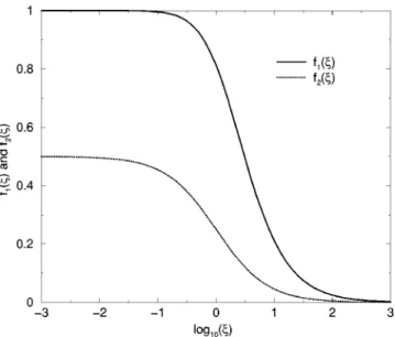
The integrations in the calculation of f₁ and f₂ above were again carried out using the calculus of residues and were checked by numerical integration. The functions f₁(j) and f2(j) are plotted in Fig. 2.

We have thus shown that a complete description of the decay out of a superdeformed band within the energy aver-age approach requires three requires three dimensionless variables,G↓_/G

S,GN/d, andGN/(GS1G↓). We find the

fol-lowing: ~1! The average contribution of the background to the intraband decay intensity,I_inav,@Eq.~46!#depends only on G↓_/G

S. ~2!The average of the fluctuation contribution,Iin fl , @Eq. ~47!# depends on two variables: G↓_/G

S andGN/d. ~3!

The variance, (DIin)2,@Eq.~55!#depends on three variables: G↓_/G

S, GN/d, andGN/(GS1G↓).

Figure 3 shows a plot of the average intraband decay in-tensityI_in@Eq.~15!#calculated using Eqs. ~46!and~47!for I_inavandI_infl. For comparison we also show theIinthat results when the GW fit formula@Eq.~49!#is used forI_infl instead of FIG. 2. The functions f1(j) @Eq. ~63!# ~solid line! and f2(j) @Eq.~64!# ~dotted line!plotted vs log10(j).

FIG. 3. Average intraband intensity I_in vs log10(bJ) where bJ

[G↓_/G

S. The filled circles were calculated using Eq.~15!together

with Eqs.~46!and ~47!. The error bars for the filled circles show

A

(DI_in)2calculated using Eq.~55!withjin the form given by Eq.

~58!. The dotted lines were calculated in the same manner as the filled circles except that GW’s fit formula, Eq.~49!, was used in the place of Eq.~47!. The variableGN/dtook the following values: 0.1

in graphs~a!,~b!, and~c!; 1 in graphs~d!,~e!, and~f!; 10 in graphs

~g!, ~h!, and ~i!. The variable G↓_/G

N took the following values:

1023_{in graphs~a!,~d!, and~g!; 1 in graphs~b!,~e!, and~h!; 10}3_in

Eq. ~47!. The two curves are barely distinguishable for G_N/d51. The GW fit formula incorrectly gives intensities that are greater than unity when GN/d50.1 as does our Eq.

~47!. The exact formula of GW @Eq. ~24!in GW#does not suffer from this problem. Our results are only strictly valid when GN/d@1.

The error bars in Fig. 3 were calculated using Eq. ~55! withj in the form given by Eq.~58!. We calculate

A

(DI_in)2 for three values of the ratioG↓_/G

N~see figure caption!. Since

(DI_in)2 is proportional toI_infl it also increases monotonically to a maximum before decrease monotonically to zero as a function of G↓_/G

S. For the same reason the error increases

monotonically with decreasing GN/d. The error estimate

presented in GW exhibits the same trends with G↓_/G

S and

GN/d.

Since the variance depends only on (GS1G↓)/GN in

ad-dition to G↓_/G

S and GN/d, upon fixing the latter two

vari-ables the variance may be considered a function of any one of G↓_/G

N, GS/GN, G↓/d, orGS/d @see Eqs.~57!and~58!#.

In Fig. 3 we chose to use Eq. ~58!forj and fixed the value ofG↓_/G

N. WhenGS/GNis fixed instead, a slightly different

dependence on G↓_/G

S is obtained @compare Eqs. ~57! and

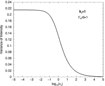
~58!#. Figure 4 shows a plot of the standard deviation,

A

(DI_in)2_{, @Eq.~55!#as a function ofG}↓_/G

Nfor fixedG↓/GS

and G_N/d. Ultimately, the variance like the intensity is a function of the spin of the decaying nucleus and could pro-vide an additional probe to the spin dependence of the barrier separating the SD and ND wells which is contained in the spreading width G↓ @5–9#.

Our result for the variance of the decay intensity (DIin)2 @Eq.~55!#has a structure reminiscent of Ericson’s expression for the variance of the cross section @17#. This connection will be fully explored in the Sec. V. For now we note only that what distinguishes Eq. ~55! from Ericson’s expression for the variance of the cross section are the functions f₁(j) and f₂(j) which result from the energy integrations in Eq. ~52!.

V. VARIANCE OF THE DECAY INTENSITY VERSUS AUTOCORRELATION FUNCTIONS OF STATISTICAL

NUCLEAR REACTION THEORY

A. Results familiar from statistical nuclear reaction theory

All moments of theS matrix,S_ab(E), the quantities that describe the way in whichSab(E) fluctuates about it’s

aver-age,Sab(E), can be expressed in terms ofSab(E) itself@19#.

Normally, specific moments such as the amplitude and cross section autocorrelation functions are expressed in terms of transmission coefficients, defined to be

Ta5Taa, 0<Ta<1, ~65!

and their generalization

Tab512

(

c

Sac Sbc*5

(

c

S_acflS_bcfl*. ~66! Here S_abfl 5Sab2Sab is the fluctuating part of the S matrix.

The transmission coefficient Ta is the probability of

trans-mission from a compound nucleus resonance to channel a and is obtained from the optical model.

In what follows we quote results for both the amplitude and cross section autocorrelation functions in the overlap-ping resonance region for the purpose of comparison with our results for the decay intensity. The amplitude autocorre-lation functionc_ab(E,E

₈

) for amplitude

Aab5dab2iSab, ~67!

is defined by

cab~E,E

8

!5Aab~E!Aab~E

8

!*2Aab~E! Aab~E

8

!*

~68!

5A_abfl ~E!A_abfl ~E

₈

!* ~69! 'sabfl

iG

E₂E

₈

₁iG. ~70!

The correlation width G is given by

G5₂d_p

(

a

Ta. ~71!

Derivation of Eq. ~70!requires the assumption thatA_ab(E)

5Aab(E

8

). This assumption together with statistical

as-sumptions equivalent to those employed in our treatment of the factor a(«) @Eq. ~32!# gives rise to acab(E,E

8

) which

depends solely on the difference of the two energies E

2E

₈

.

Equation ~44!, which is essentially c00(E,E

8

) does not depend solely onE₂E

₈

. The background energy modulation in bothEandE

₈

which is characteristic of an isolated door-way resonance is explicit. In the present case it cannot be assumed that A₀₀(E)ÞA₀₀(E

₈

) for arbitraryE andE

₈

. The double integral for the variance of the decay intensity @Eq. FIG. 4. The standard deviation of the decay intensity

A

(DIin)2

vs log10(cJ), wherecJ[G↓/GNplotted using Eq.~55!withjin the

form given by Eq.~58!for fixedbJ5G

↓

~52!and Eq.~77!below#is sensitive to this fact as it contains products of the background amplitudes at arbitraryEandE

₈

. The amplitude autocorrelation function, Eq.~44!, contains two distinct energy dependences, one characterized by G_N which is analogous to Ericson’s correlation width as defined by Eq.~71! and another characterized byGS1G↓ the width

of the doorway. Writing Eq.~44!in terms ofxandx

₈

defined by Eqs.~53!and~54!

c₀₀~E,E

₈

!516_jiI_inavI_infl 1

@x₁i#2@x₂x

₈

₁2i/j#@x

₈

₂i#2, ~72!

we see that it in fact depends only on the ratio GN/(GS

1G↓_{) and it is through Eq.~44!that this variable enters our}

calculation of the variance of the decay intensity.

The amplitude autocorrelation function is not an observ-able quantity. The correlation width, Eq. ~71!, must be ex-tracted from correlation analysis of the cross section. The cross section autocorrelation function, C_ab(E,E

₈

), for cross section sab5uAabu2 is defined by

Cab~E,E

8

!5sab~E!sab~E

8

!2sab~E! sab~E

8

! ~73!

'ucab~E,E

8

!u2

12 ReAab~E!*cab~E,E

8

!Aab~E

8

! ~74!

'@sabfl 212sab

av_s

ab

fl

# G

2 ~E₂E

₈

!2₁G2.

~75!

Here,sab

av

5uAabu2 is the background cross section. The

fluc-tuation contribution to the cross section in terms of the trans-mission coefficients is given by the Hauser-Feshbach for-mula

sab

fl _' TaTb

(

_c T_c

, ~76!

or some modification of it designed to account of width fluc-tuations, direct reactions, etc.@15,20#.

Equation ~52! for the variance of the decay intensity can be written in terms of the cross section autocorrelation func-tion defined by Eq.~74!as

~ DI_in!25~2pG_S!22

E

2` `

dE

E

2` `

dE

₈

C₀₀~E,E

₈

!. ~77!

The same comments concerning the energy independence of the background amplitude apply to the derivation of Eq.~75! as applied to the derivation of Eq.~70!. LikewiseC₀₀(E,E

₈

) in the case of the present paper@the integrand in Eq.~52!#is distinguished from Eq. ~75! by its explicit inclusion of the energy dependence of the background. Equation ~52! and ~74!assume that only pairwise correlations are present. Both

Eqs. ~70! and ~75!are valid when (aTa@1, that is, in the

strongly overlapping resonance region.

B. Expression of the decay intensity and variance in terms of transmission coefficients

Following GW we introduce two transmission coeffi-cients,T₀(E) andTN, where

T0~E!512uS00u25

G_SG↓

~E₂E₀!21~ GS1G

↓

!/4 ~78!

5

4I_inav~1₂I_inav! 4~E2E0!2/~ GS1G

↓

!11 ~79!

describes transmission from theuQ

&

to the SD band and

TN52pGN/d ~80!

describes their transmission to ND states of lower spin. We have not derived Eq. ~80!. For the purposes of the present paper it can be taken as the definition of TN. The reader is

referred to the discussion in Sec. VIII H of Ref. @21#which contrasts the relation of the correlation widthG to transmis-sion coefficients with the the corresponding relation for the average widthGq.

We have writtenT₀(E) in the form given by Eq. ~79!in order to emphasise that it isnotsimply a function of a single dimensionless variable, the ratioG↓_/G

S. It is energy

depen-dent, the energy dependence being characterized by G_S

1G↓_{, the total width of doorway stateu0}

_&

_{. Only it’s}

maxi-mumT₀(E₀)₅4I_inav(1₂I_inav) can be expressed solely in terms of G↓_/G

S. Thus, a quantity sensitive to the gross energy

dependence ofT₀(E) should depend onG_S1G↓

. Writing the average decay intensity Eq.~15!in terms transmission coef-ficients

Iin512~2pGS!21

E

2`

`

dE$T0~E!22@T0~E!#2/TN%,

~81!

we see that it compares the total width of the doorway u0

&

with the width for the feeding of u0

&

@thanks to inclusion of the normalization factor 2pGS in the definition ofIinin Eq. ~1!#. The variance, Eq.~52!, may be written as

~ DIin!2

'~2pGS!22

E

2`

`

dE

E

2` `

dE

₈

H

4T0~E! 2_T

0~E

8

!2 @2p~E2E

₈

!/d#21TN2

14 ImA00~E!T0~E!T0~E

8

!A00~E

8

!* 2p~E₂E

₈

!/d₁iTN

J

. ~82!

two characteristic energy scales in fact only depends on their ratio,GN/(GS1G↓), the ratio of the correlation width to the

doorway width.

Equation~41!may also be expressed in terms of the trans-mission coefficients T0(E) and TN. Using Eq. ~43! for G↑

we get

G₅ d

2pTN

F

12

T₀~E!/T_N

I_inav

G

, ~83!

so that the neglect of G↑ _{in G is justified when T}

0(E)/TN

!I_inav<1. Let us also write the correlation lengthj, Eq.~56!, in terms of the transmission coefficients

j5~2p/TN!

GS1G↓

d . ~84!

In the case of compound nucleus scattering, extraction ofG from a measurement of cross section autocorrelation func-tion, using say Eq. ~75!, permits the determination of the density of compound nucleus states 1/dby application of Eq. ~71! @22#. A more recent example of energy-autocorrelation analysis may be found in Ref. @23# where fluctuations in dissipative binary heavy ion collisions are studied. In the present case of the decay out of a superdeformed band ex-traction of j from the variance of the intensity, permits the determination of the ratio (GS1G↓)/GN, or, given TN

~equivalently GN/d) determination of the ratio (GS

1G↓_)/d.

C. Comparison with the results of Gu and Weidenmu¨ller

GW also take inspiration from statistical nuclear reaction theory but use the MPI approach@24#. The MPI approach is concerned with the analytic calculation of ensemble aver-ages, a procedure which is equivalent to the calculation of energy averages. Reference @24# use the supersymmetry method of calculating ensemble averages to derive an exact expression for S_abfl (E)S_cdfl (E

₈

). Their result is found to be expressible in terms of the difference of the two energies, E₂E

₈

, and transmission coefficients. The transmission co-efficients themselves are expressed as functions of (E

1E

₈

)/2. The relationship between the results of@15–17#and those of Ref. @24# is discussed in Refs.@20,25#. Several re-sults of Refs.@15–17#can be obtained from that of Ref.@24# by expanding in powers of the transmission coefficients or inverse powers of the sum of the transmission coefficients @20#.

Calculation of the average of the fluctuation intensity re-quires the energy integral of the average of the product of two S-matrix elements at the same energy. GW use the re-sults of Ref.@24#foruS₀₀fl(E)u2_{to calculate the average decay} intensity. As was already noted in Sec. III, GW include the energy dependence of the background amplitude characteris-tic of an isolated doorway resonance in their calculation by using the energy dependent transmission coefficient T₀(E), Eq. ~78!, in their Eq. ~24! for I_infl. The fact that we use the same energy dependence as GW for the background is

re-sponsible for the agreement we obtain with GW concerning I_in’s dependence onG↓_/G

S. The differences between our

re-sults and those of GW for the decay intensity stem from the assumptions we make which restrict our results to G_N/d

@1.

Calculation of the variance of the intensity requires the four-point function at two energies integrated over both en-ergies, that is, it requires S₀₀fl(E)S₀₀fl(E)*S₀₀fl(E

₈

)S₀₀fl(E

₈

)*

integrated overEandE

₈

. Calculation of the four-point func-tion at two energies was carried out using the supersymmetry method in Ref.@26#. Their result, like that of Ref.@24#for the two-point function depends explicitly only onE₂E

₈

and the transmission coefficients which are again expressed as func-tions of (E₁E

₈

)/2. Within the assumption that only pairwise correlations are important, as was assumed in Eqs.~52!and ~74!, the two-point function is enough to calculate the vari-ance. Reference @20#showed numerically that the exact ex-pression of Ref.@24#specialized to the amplitude autocorre-lation function confirms the correctness of Eq. ~70! in the region of strongly overlapping resonances. However, unlike Eq. ~70!, the amplitude autocorrelation function as given by Eq.~44!depends on the background amplitude at two differ-ent energies, that is, it depends on A₀₀(E) and A₀₀(E

₈

). WhenE₅E

₈

it reduces to Eq.~45!which can be expressed in terms of the transmission coefficientsT₀(E) andT_N. Thus the decay intensity can be expressed in terms of these trans-mission coefficients as was done in Eq.~81!. The applicabil-ity of Ref. @24# to calculation of the decay intensity owes itself to the fact that the decay intensity may be expressed in terms of transmission coefficients.

Equation ~44! cannot be written in terms of T₀(@E

1E

₈

#/2) and the same applies to the variance as is apparent from Eq.~82!. Thus it is not clear whether Ref.@24#serves as a means to obtain results corresponding to Eqs.~44!and~82! which are valid for arbitrary GN/d. It would be an

interest-ing challenge to derive an expression for the variance which could be used for any value of GN/d since for the regions

which have been most frequently studied experimentally@2#, the A'150 andA'190 regions,G_N/d!1.

GW do not use the supersymmetry method to calculate the variance. They instead estimate the variance by perform-ing a numerical simulation. The analytic structure of the vari-ance was not investigated in GW and their results make no reference to the variable GN/(GS1G↓). Given the close

re-semblance of the conclusions about the analytic structure of the decay intensity which may be inferred from the exact result of GW and our approximate result for GN/d@1 it

seems probable that the dependence of the variance on G_N/(G_S1G↓

) which we have found for G_N/d_@1 persists for arbitraryGN/d.

VI. CONCLUSIONS

Eq. ~55! for the variance (DIin)2 were derived by making assumptions and approximations which are strictly valid only in the strongly overlapping resonance region, GN/d@1.

However, these formulas are seen from Figs. 2 and 3 to work well when GN/d51 and provide a qualitative description

even when G_N/d₅0.1. This means that Eq. ~47! and Eq. ~55! cannot be applied to the mass 150 and 190 regions whereGN/d;0.001 but they may prove themselves of

prac-tical use in other mass regions. In any case our results clarify the analytic structure of the results obtained by GW. In par-ticular we have revealed that the variance of the decay

inten-sity depends on the correlation lengthGN/(GS1G↓) in

addi-tion to the two dimensionless variables G↓_/G

S andGN/d on

which the average of the decay intensity depends. Measure-ment of the variance of the decay intensity could yield the mean level density of the ND states in analogy with autocor-relation analysis of cross sections.

ACKNOWLEDGMENTS

This work was partially supported by FAPESP.

@1#T. Lauritsenet al., Phys. Rev. Lett.88, 042501~2002!.

@2#A. Lopez-Martenset al., Phys. Scr.T88, 28~2000!.

@3#A. Dewaldet al., Phys. Rev. C64, 054309~2001!.

@4#R. Krucken, A. Dewald, P. von Brentano, and H.A. Weiden-muller, Phys. Rev. C64, 064316~2001!.

@5#E. Vigezzi, R.A. Broglia, and T. Dossing, Phys. Lett. B249, 163~1990!; Nucl. Phys.A520, 179c~1990!.

@6#Y.R. Shimizu, F. Barranco, R.A. Broglia, T. Dossing, and E. Vigezzi, Phys. Lett. B274, 253~1992!.

@7#Y.R. Shimuzu, E. Vigezzi, T. Dossing, and R. Broglia, Nucl. Phys.A557, 99c~1993!.

@8#Y.R. Shimizu, M. Matsuo, and K. Yoshida, Nucl. Phys.A682, 464c~2001!.

@9#K. Yoshida, M. Matsuo, and Y.R. Shimizu, Nucl. Phys.A696, 85~2001!.

@10#S. Aberg, Phys. Rev. Lett.82, 299~1999!; Nucl. Phys.A649, 392c~1999!.

@11#R. Krucken, Phys. Rev. C62, 061302~R! ~2000!.

@12#A.J. Sargeant, M.S. Hussein, M.P. Pato, N. Takigawa, and M. Ueda, Phys. Rev. C65, 024302~2002!.

@13#J.z. Gu and H.A. Weidenmuller, Nucl. Phys.A660, 197~1999!.

@14#H.A. Weidenmuller, P. von Brentano, and B.R. Barrett, Phys. Rev. Lett.81, 3603~1998!.

@15#H. Feshbach,Theoretical Nuclear Physics: Nuclear Reactions

~Wiley, New York, 1992!, Chap. IV.

@16#M. Kawai, A.K. Kerman, and K.W. McVoy, Ann. Phys.~N.Y.!

75, 156~1973!.

@17#T. Ericson, Ann. Phys.~N.Y.!23, 390~1963!.

@18#P. R. Wallace, Mathematical Analysis of Physical Problems

~Dover, New York, 1984!, Chap. VIII.

@19#J. Richert, M.H. Simbel, and H.A. Weidenmuller, Z. Phys. A 273, 195~1975!.

@20#J.J. Verbaarschot, Ann. Phys.~N.Y.!168, 368~1986!.

@21#T.A. Brody, J. Flores, J.B. French, P.A. Mello, A. Pandey, and S.S.M. Wong, Rev. Mod. Phys.53, 385~1981!.

@22#T. Ericson and T. Mayer-Kuckuk, Annu. Rev. Nucl. Sci. 16, 183~1966!.

@23#M. Papaet al., Phys. Rev. C61, 044614~2000!.

@24#J.J. Verbaarschot, H.A. Weidenmuller, and M.R. Zirnbauer, Phys. Rep.129, 367~1985!.

@25#Y. Takahashi and S. Yoshida, Nucl. Phys.A507, 371~1990!.