SLOSHING PHENOMENA IN TANKS
DUE TO LONG PERIOD-LONG
DURATION HARMONIC MOTIONS
ALI VAKILAZADSARABI
Civil Eng. Dept., Faculty of Natural Scs. and Technology, Kanazawa University Kakuma Machi, Kanazawa, Ishikawa 920-1192, Japan
MASAKATSU MIYAJIMA
Civil Eng. Dept., Faculty of Natural Scs. and Technology, Kanazawa University Kakuma Machi, Kanazawa, Ishikawa 920-1192, Japan
Abstract:
Long period –long duration ground motions have come to bean important consideration because of the recent rapid increase in the number of structures such as storage tanks, high rise buildings and suspension bridges. Most long-period ground motions were generated by large earthquakes and effective propagation paths, such as accretionary prisms. Also in liquid tanks, most damage during earthquakes occur due to liquid sloshing, especially during long period and long duration ground motions. For this purpose, in this paper the three-dimensional fluid structure interaction simulation is applied to study the effect of motions inside a sloshing tank. An improved CEL and SPH techniques are used to assure an accurate description of water displacement and the pressure on the walls. Nonlinear computational results are validated and compared with linear analytical and experimental results to obtain some useful insight into the effect of period and duration of motions on the sloshing phenomena in water tanks.
Keywords: sloshing, water reservoir, long period-long duration, numerical analysis, CEL, SPH. 1. Introduction
One of the demanding lifeline structures which have become widespread using during the recent years is a liquid storage tank. These structures are widely used in water supply facilities, gas and oil industries and nuclear plants for storage of a variety of liquid or liquid-like materials such as oil, liquid natural gas, chemical fluids and other forms. Issues associated with liquid tanks involve many essential problems. The calculation of hydrodynamic forces on the wall of vibrating liquid tanks is an important issue of preserving the structure of tanks and vessels.
Sloshing means any motion of the free liquid surface inside tanks. It is affected by disturbance to partially filled liquid containers. Basically, liquid sloshing on the free surface may have serious influence on the response of the tank. The basic problem of liquid sloshing includes the estimation of the hydrodynamic pressure, forces, moments and natural frequencies of the free liquid surface. These criteria have a straightforward effect on the dynamic stability and performance of moving tanks. Commonly, the hydrodynamic pressure of liquids in moving tanks has two noticeable factors. One factor is directly corresponding to the acceleration of the tank. This is caused by the part of the fluid moving with the same tank velocity. The second factor is known as convective pressure and represents the free surface liquid motion. Mechanical models such as a mass spring dashpot or pendulum systems are usually used to model the sloshing part. Sloshing waves have been studied numerically, theoretically and experimentally in the past several decades and many significant phenomena have been considered in those studies, especially the linear and nonlinear effects of sloshing for both inviscid and viscous liquids.
Modelling of new arisen engineering problems has evident effect in their solving evolution. And earlier researchers, who is dealing with a too unknown problem to be solved in a direct full analytical way, use reasonable simplicity assumptions to reduce the physical concept of the event to simple and rough analytical model which can be described by initial known principles without any considerable deficiency occurrence in the original problem.
continue alternatively between analytical and numerical models until finding a reasonably exact one and finally, the principal establishment for considering an event. Modelling of sloshing, as an estimated and complicated engineering event, has a similar unfinished evolution process and herein two new computational procedures utilizing CEL and SPH techniques are used to solve fluid structure interaction problems with free surface. The procedure of these methods is explained shortly and concerning fluid-structure equations are explained. These numerical methods are applied to small scale tanks subjected to external excitations, and the results validated on tank models using the experimental and analytical methods in terms of height of the water free surface.
2. Experimental setup
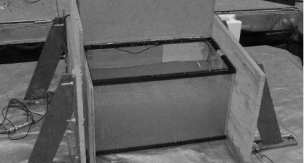
Major A brief explanationof the experimental setup is provided. The sloshing experiments are carried out in a rectangular tank partially filled with colored water at the atmospheric and room temperature. The tank dimensions are . . . , corresponding to the length, height and width of the tank. The dimensions of the tank are chosen to ensure a three dimensional flow. The walls are made of transparent Plexiglas for optical access. The tank is mounted on top of a motion system with six degrees of freedom. Figure.1 shows the experimental setup. For the experiment mentioned here, the tank was filled 64% with water corresponding to H=0.23 m. The tank is excited by a horizontal acceleration sin in which
. m. s and frequency of 0.4 Hz and 0.8Hz, which are non-resonant frequenciesand 1.042 Hz, which is
resonant frequency in duration of 60 seconds.
Fig. 1. Experimental setupwhich has done in the shaking table of earthquake engineering laboratory of Kanazawa University
3. Numerical modeling
The fundamental governing equations of sloshing are based on the following two essential physical conservation laws:
Continuity equation as:
div (1)
Momentum equation as:
grad (2)
where is the density of fluid, t is the time, ν is the velocity vector of the fluid particle, P is the pressure of the fluid, , are, respectively, the horizontal and vertical exciting accelerationand g is the gravity acceleration. is the diffusion term which is related to the viscosity of the fluid.
In this paper the hydrodynamic response of the water is modelled with the equation of state (EOS) materials, thatdefines the material’s volumetric strength and pressure to density ratio. As a fluidinfluences a solid body, a complex pressure field is formed in the influenced region. The first phasecontains the peak pressure value (Hugoniot pressure) having the below theoretical value:
/ (3)
while ρ as the material initial density, where U phase and U0 are the shock and impact velocities, respectively (Wilbeck, 1977). The maximum pressure is driven by a pressure phase, and the final phase is expressed by the establishment of a steady flow pressure, having a constant but a much lower value:
(4)
Pitot pressure or Stagnation pressurevalues are predictable, despite the Hugoniot pressure which depends on the shock velocity, also it is a function of the velocity. In addition,via the Mie-Grüneisen equation, water has been assumed as an incompressible fluid. The linear Mie-Grüneisen equation also called US–UP equation of
(5)
where c0 is the speed of sound in the material and s is a material constant. The final form of pressure to density
relation is determined by:
(6)
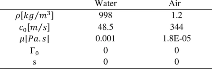
whereΓ0 is material constant, η = 1 −ρ0/ρ is the nominal volumetric compressive strain, and E is the internal energy per unit mass. To define the EOS material only four material properties need to be statedρ0, c0, Γ0 and s. Since an expanded literature survey, for this work the linear equation of state is used, and to minimize simulation run time, with a wave speed of c0 = 48.5 m/s, s = 0, Γ0 = 0, and a density of
kg. m were used.The wave speed corresponds to a bulk modulus of 2.07 MPa, three orders of magnitude
less than the actual bulk modulus of water. The results compare very well between the simulation with the actual wave and the simulation with the reduced wave speed. Alsothe dynamic viscosity of water is chosen as 0.001.The Mechanical properties of water listed in Table 1.
Table 1.Values of parameters used to model water and air
Water Air
⁄ 998 1.2
⁄ 48.5 344
. 0.001 1.8E-05
Γ 0 0
s 0 0
3.1. CEL modeling
A pure Lagrangian analysis does not perfect because of excessive distortion in various elements and the defined contact cannot be acted correctly because of large distortion of the elements. The other choice to construct undistorted mesh is to use Coupled Eulerian-Lagrangian (CEL)method which controls mesh geometry from material geometry. In spite of a Lagrangian method,the structure of the mesh is related to obtaining a homogeneous and undistorted mesh. The accuracy of a CEL calculation has been often higher than the accuracy of a Lagrangian because the algorithms used to remap the solution from the distorted to the undistorted mesh is second order advection algorithms, while the algorithms in Lagrangian method for the remap in the reasoning is only first order accurate.
The futures of the CEL method are described in detail in earlier works by Souli (2011). CEL method is a technique that combines features of Lagrangian and Eulerian within the similarportion. CEL, was suggested by Noh (1964) and Hirt et al.,generally used to control element distortion in Lagrangian parts which have large deformations, such as sloshing analysis. Most CEL analyses can also be done as pure Eulerian analyses, but some of the features dealing with a Lagrangian mesh will be lost. CEL is a way that by allowing the mesh to move independently of the material makes it possible to preserve a high quality mesh during an analysis, even as the excessive deformation or loss of material occurs. CEL meshing does not change the topology (elements and connectivity) of the mesh, which involves some limitations on the capability of this method to preserve a high quality mesh upon extreme deformation.
The equilibrium equations for fluid and structure are formulated with three equations of energy, momentum and mass. Although fluid and structure are governed by the same balance equations, the consulting equations, which express the material behavior and related stress to estimate deformation of two materials, are different.
In the CEL method, while material passes between elements of the computational mesh, the density is required to be balanced explicitly to account for the conservation of mass during the non-Lagrangian deformation. The equation of mass conservation for an incompressible Newtonian fluid in the CEL method is given by:
div grad (7)
The momentum equation as:
grad (8)
The total energy equation for the CEL is expressed as:
Where is the density,e is the internal energy per unit volume, is the strain rate tensor, is the body force, andt is time. Total Cauchy stress, σ, is defined as the sum of the deviatoricstress andpressure:
Id (10)
whereP is the pressure,Id is the identify tensor, and is the dynamic viscosity of the fluid.Although any of the Lagrangian, Eulerian or CEL algorithms can be used to model the fluid motion for fluid-structure interaction problems, the structure is always discretized with Lagrangian approach. Since in Lagrangian algorithm computational mesh nodes always follow the associated points of the material domain during motion, the advection term does not exist. Momentum and energy equations for Lagrangian algorithms can be given as follows respectively:
div (11)
: (12)
where σis the total Cauchy stress given by:
Id (13)
In this case G represents shear modulus and, ε is shear strain.
3.1.1. Boundary conditions
In fact, boundary conditions are related to the problem, not to the description employed. Thus, the same boundary conditions employed in Eulerian or Lagrangian descriptions are implemented in the CEformulationion, that is along the boundary of the domain, kinematical and dynamical conditions must be specified. Generally, this is described as:
Γ
. Γ (14)
where and t are the prescribed boundary velocities and tractions respectively; n is the outward unit normal to Γ , and Γ and Γ are the Derichle and Neumann different subsets respectively, which explain the piecewise smooth boundary of the target domain. Usually, stress conditions at the boundaries represent the natural boundary conditions, and therefore, they are directly considering in the weak form of the momentum conservation equation. If part of the boundary is composed of a material surface whose position is unknown, and then a mixture of both conditions is required. The CEL formulation allows an accurate tracking of material surfaces.
In a custom Lagrangian analysis, nodes are fixed inside the material, and elements distort as the material distorts. Lagrangian elements are always totally full of a single material, so the material boundary overlaps with an element boundary.
By contrast, in an Eulerian analysis, nodes are fixed in space, and materialruns through elements that do not distort. Eulerian elements may not always betotally full of material; several may be partially or completely void.Therefore,the Eulerian material boundary must, be computed during each time increment and generally does not correspond to an element boundary. The Eulerian mesh is typically a simple rectangular grid of elements created to cover well beyond the Eulerianmaterial boundaries, giving the material space in which to move and deform. In fact, if some Eulerian material passes outside the Eulerian mesh domain, it is lost from the simulation. Eulerian material can interact with Lagrangian elements through Eulerian–Lagrangian contact. Volume fraction data are computed for each Eulerian material in an element. Within each time increment, the boundaries of each Eulerian material are reconstructed using these data. The interface reform algorithm approaches the material boundaries within an element as simple planar surfaces; considering thatthe Eulerian method is applied only to three-dimensional elements. This assumption produces a simple, estimated material surface that may be discontinuous between neighboring elements. Therefore, accuratedetermination of a material’s location within an elementis possible only for simple geometries, and finemesh resolution is required in most Eulerian analyses.
The material representing the water can fall during the analysis, and the mesh does not need to adjust to the topology of the materials; in fact, a simple rectangular grid typically provides the best outcomes.
target object. This can greatly reduce the mesh size required and, hence, the simulation solution time and cost. An Eulerian section assignment defines the materials that may be present in the network over the advancement of the analysis, and an initial condition specifies which materials are present in each element at the start of the analysis. The initial condition effectively governs the initial topology of the materials in the model. The water inside the tank has been included into the model by defining an Eulerian initialized with water.In this numerical analysis the Eulerian material is tracked as it flows through the mesh by computing its Eulerian volume fraction (EVF). Each Eulerian element is designated a percentage, which represents the portion of that element filled with a material. If an Eulerian element is completely filled with a material, its EVF is 1; if there is no material in the element, its EVF is 0. Contact between Eulerian materials and Lagrangian materials is enforced using a general contract that is based on a penalty contact method. A general contact algorithm does not enforce contact between the Lagrangian elements and the Eulerian elements. The Lagrangian elements can be given through the Eulerian mesh without resistance until they bring on an Eulerian element filled with material (EVF ≠ 0).The water inside the tank has been included into the model by defining an Eulerian initialized with water.The tank structure can be modeled using traditional nonlinear Lagrangian elements. The Eulerian-Lagrangian contact formulation is based on the enhanced immersed boundary method. A great benefit of thismethod is there is no penury to make a conforming mesh for the Eulerian domain. A rough property is introduced into a mechanical surface model governing the interaction of the contact surfaces.
The impacting forces and pressures exerted during the impact are transferred to the flap model by the use of general contact algorithms. The contract is created between Lagrangian mesh surfaces and Eulerian material surfaces, which are automatically computed and tracked during the analysis. In this researchPenalty contact algorithms to introduce coupling between Eulerian and Lagrangian instances, as this approach uses the smallest computational effort and gives greater robustness.
3.2.SPH modeling
Smoothed Particle Hydrodynamics (SPH) is a numerical method which is part of the family of mesh-less or mesh free methods. It was proposed by Gingold and Monaghan (1977) primarily for astrophysical problems. This method is based on Lagrangian method wherever the coordinates move with fluid, and the resolution of the method can be adjusted regarding inconstant such as density. There are many purposes for which both the Lagrangian and the smoothed particle hydrodynamics methods can be used. In many Eulerian-Lagrangian analyses the material to void ratio small and, therefore, the calculative effort might be excessively high. In such a these cases the smoothed particle hydrodynamics method can be useful. For the application of SPH into incompressible flow (such as water) the continuity equation can be written in two forms:
∑ (15)
or by:
∑ . (16)
where a is the particle of interest, b is the neighboring particle by particle a, is the particle density, m is the particle mass, w is the kernel function and is the
city difference of particles a and b. is the kernel function which has the features of symmetric, normalization, monotonic, and compact support. Eq. (16) preferred because it shows a less boundary insufficiency error than Eq. (15).
The SPH momentum equation is shown in Eq. (17) which Π is the viscosity term.
∑ (17)
For water simulations, Cleary (1998) viscosity model is chosen because this model, angular momentum assuming smoothing length h remains constant:
(18)
where is the dynamic viscosity of the fluid and numerical calibration yields . (Cleary, 1998). The force per unit mass appearing from a boundary particle in a fluid particle within a close domain is:
(19)
where B is the reference pressure defined as ⁄ . Based on experimental data, Cole suggested B=3047 MPa and . for water. (Table.1)
When a fluid particle is coming close to a closed boundary, it is supposed to be blocked. A water particle near a wall still has the density and other quantities of water. Three boundary condition theories are used in the SPH method, which are ghost boundary condition, repulsive boundary condition and dynamic boundary condition. The ghost boundary condition was proposed by Randles and Libersky (1996). In this method the properties, including particleposition, vary with each time step to prevent particles from penetrating through the boundaries. Based on the repulsive boundary condition, fluid particle can never cross a solid boundary (Monaghan 1994; Monaghan and Kos; Rogers and Dalrymple 2008). The dynamic boundary particles; which are applied in this research, were proposed by Dalrymple and Knio (2000) and developed by Crespo et al. (2007). The boundary shares the same properties as the fluid particles. They have to satisfy the same equations of state, continuity and energy equations.
In this technique the fluid is modeled by using continuum pseudo-particle.As the internally determined connectivity is permitted to change every increment, the method robustly handles the severe deformations associate with the water disturbution. The smoothed particle hydrodynamics methodapplied in this research uses a cubic spline as the interpolation polynomial and is based on the classical smoothed particle hydrodynamic theory as mentioned before.These particle elements utilizethe existing functionalityto reference element-related features such as materials, initial conditions, distributed loads, and conception. These one node elements fill only the space initially occupied by the water just before the impact. Therefore, less elements are necessary when compared to the number of Eulerian elements in the CEL method. There are no hourglass or distortion control forces associated with these elements. These elements do not have faces or edges associated with them. Also a node-based surface associated with the water, pseudo-particle; is included in the contact domain to model the interaction between the water and the tank.
4. Analytical formulations for sloshing in tank subjected to harmonic motion
A tank problem with sloshing liquid is generally regarded as an initial boundaryvalue problem. The sloshing of irrotational flow of an incompressible and inviscid fluid within a container is treated by potential flow theory in which the motion of the fluid inside a tank governed by the Laplace equation:
(20)
where represents the velocity potential function of fluid. It is possible to split the total velocity potential function, , into a fluid disturbance potential function, , and a potential function, , which defines the motion of the tank, that is:
(21)
The tank is excited in the lateral direction using the following sinusoidal function with a driving frequency
:
χ t sin (22)
where represents the harmonic external force amplitude. The tank potential function defines the motion of the tank and computed by the following equation:
cos (23)
With reference to Fig. …, Graham and Rodriguez (1974) solved the three dimensional velocity potential:
, , , ∑∞ ∑∞ cos cos (24)
where L and l are the tank width and breadth, respectively, , m and n are positive
integers. The corresponding free-surface natural frequency is:
tanh (25)
The wave height, can be written in the form:
, , (26)
It measured from the undisturbed liquid surface at equilibrium, and pressure can be defined in terms of velocity potential function as follows:
, , , (27)
5. Results for sloshing in the tank due to horizontal excitation
The results of numerical and analytical methods which is presented in this paper are compared together and they verified with experiments in order to determine the applicability of the developed analysis of sloshing problem, which is done at the shaking table laboratory of the earthquake engineering of the Kanazawa university in terms of free surface profile and wave height. The shaking table was small scale, but it can be controlled to apply sinusoidal, pulse and random motions in two directions.
5.1.Free surface profiles
In view of the limitation of numerical modeling, a small scale 3D model is built to investigate the fluid free surface profile under horizontal sinusoidal acceleration motion. The scaled glass made rectangular tank model is fabricated with a width of 0.6 m, a breath of 0.3 m, height of 0.36 m and a thickness of 0.01 m. Water level is 0.23 m inside the tank. From Eq. (25) the first natural sloshing frequencies for this tank is calculated as . Hz. Three harmonic tests are conducted to apply sinusoidal motion with acceleration amplitude of . ⁄ and non-resonant frequencies of 0.4 Hz, and 0.8Hz and 1.042 Hz which is the resonant frequency.
The sloshing event inside a 3D tank subjected to harmonic motion is investigated with fully nonlinear fluid-structure interaction algorithm based on CEL approach and SPH methods implemented in this paper. The free surface profiles of the rectangular tank model obtained from experimental and numerical studies are compared at an arbitrary instant for each loading case.
The tank is modeled as 3D in the shape of rectangles in the numerical simulations both CEL and SPH methods. Rigid solid elements are used for tank walls and Eulerian mesh for the fluid domain in CEL method and Lagrangian particles to simulate fluid in SPH method are used. The Eulerian meshes of the CEL consist of 81920 Eulerianelements with the dimension of 0.01m and the solid Lagrangian mesh consist of 12560 elements with the dimension of 0.01 m in all directions. Also in SPH method the number of particles consist are 41400 particles. The water assumed that was incompressible and invoiced elastic fluid material. Boundary condition of experimental analysis and numerical analysis was chosen to be same.The slosh event simulated for this water tank system in 60 seconds using a velocity time history. The Eulerian mesh motion is engaged to allow the Eulerian mesh to move in space to surround the water tank.The simulation carried out on a Windows/x86-64 platform with 8 CPUs. The simulations took about 230 hours to solve for one analysis.
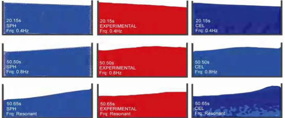
The comparison of the results of the studies is shown in Figure 2 at three different times of 20.15s, 50.50 s and 50.65 s for the situation of when the amplitude and frequency of the applied harmonic acceleration are
. ⁄ ,0.8 Hz, and resonant frequency respectively. This figure shows that the free surface profile obtained
from an experimental study matches with the numerical analysis.
Fig. 2. Free surface profiles of SPH, Experimental and CEL models under sinusoidal excitation with amplitude of 0.4 m.s-2 at different
times.
5.2.Sloshing wave height and pressure
Water displacement inside the tank subjected to harmonic motion is studied in this part considering the nonlinear interaction of water and rigid tank based on CEL and SPH approaches. These numerical results are compared with with the related results of experimental and analytical formulations. Shaking table results is reference solution for this problem. The physical properties and boundary conditions of model are same as the last part. In numerical methods the time step size is 0.01 s throughout the simulation.
taken asthe same as first fundamental frequency. The amplitudesof the horizontal harmonic excitations are
. . forall cases. The time history response of free surface elevationis measured at three locations which
were near left(i.e. x = −0.3) and right (i.e. x = 0.3) ends of the tank.
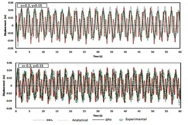
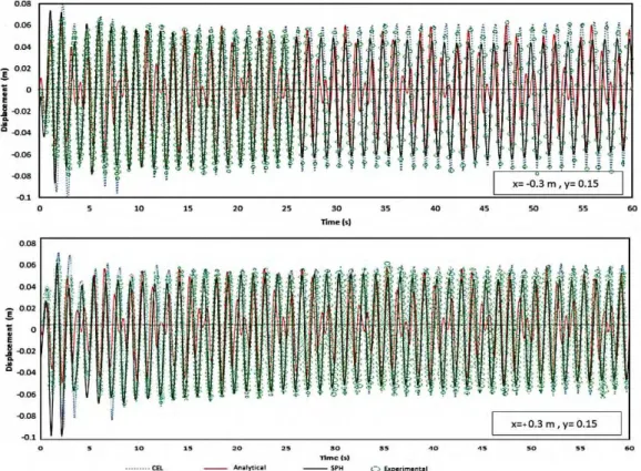
In case of non-resonant frequency motion, the numerical solutionof sloshing by the proposed methods (CEL and SPH) is in a acceptable agreement with the reference solution and analyticalformulation in terms of displacement of water surface.Corresponding to the frequency of 0.4 Hz, figure 3shows the time history response of freesurface elevations at two measurement locations (i.e.x = −0.3, 0 and 0.3 m) that is extended to 60 s. Themaximum sloshing amplitude at x = -0.3 m is measuredas 0.052 m from the CEL solution and 0.051 from the SPH solution, whereas,it is obtained as 0.053m from both the analyticalformulation and experimental data. Theminimum free surface elevation is obtained as 0.050 m,0.051 m, 0.054 m and 0.048 from experimental, analytical,CEL and SPH methods, respectively. In both cases, the numericalresults are quite close to the experimental ones.
Fig. 3. Time histories of sloshing wave height two end points obtained by CEL, Analytical, SPH and experimental methods with the frequency of 0.4 Hz
Fig. 4. Time histories of sloshing wave height two end points obtained by CEL, Analytical, SPH and experimental methods with frequency of 0.8 Hz
In the case of resonant frequencythat is extended to 10 s, Figure(5) presents the wave height increasescontinuously for all solution types atthe near left and right end of the tank. The comparisonof four solution methods shows that analytical studyoverestimates surface amplitudes. Numerical and experimentalresults are highly consistent in terms of peaklevel timing, shape and amplitude of sloshing wave.The free surface displacement time histories obtained fromexperimentaland numericalstudies show that the upward sloshing wave amplitudes are always superior thanthe downward ones. This phenomenon is a sign of a nonlinear behavior of sloshing andcaused by the suppression effect of the tank base on waveswith downward amplitude. Although the gravity effects existfor upward and downward fluid motion, the downwardmotion of fluid is obstructed by the tank bottom. The ratioof positive amplitude to absolute negative amplitude increasesas the fluid depth decreases. This iscannot be perceived from the analytical solution because it is derived based on linearized assumptions.
Press −0. 3) an resonant measured hydrostat is ahigh frequency numerica hydrodyn
Fig. 6. Pre
Fig. 7. Pre
sure time histo nd right (x = 0 (0.4 and 0.8 H d in the exp
tic pressure fi frequency os y motion, the al methods at t namic pressur
essure time histor
essure time histor
ories, includin 0.3) sides of t Hz) andfigure perimental stu
eld is generat scillation regi ere is a smal the left and ri e to total pres
ries at two end loc
ries at two end lo
ng hydrodynam the tankabout e (8) for resona
udy, only an ted by increasi ion in pressur ll phase diffe ght sides of th ssure response
cation of the tank
cation of the tank
mic pressure,d 0.01 m above ant frequency nalyticaland n
ing the gravity re response in erence in pre he tank. For n e is very small
k wall obtained by Hz
k wall obtained by Hz.
detected at tw e the baseare y motions, resp
numerical re ygradually in n the first 5 essure time hi non-resonant fr
l value.
y CEL, Analytica
y CEL, Analytica
wo locations w plotted in Fig pectively. Sin
sults are com the first secon s of the anal istories obser frequency mot
al and SPH metho
al and SPH metho
which are on th gures (6)and(7 ce the pressur mpared. Alth nd of the anal lysis. For non rved by analy tion, the contr
ods with the frequ
ods with the frequ
heleft (x = 7) fornon-re was not hough the
lysis there n-resonant ytical and ribution of
uency of 0.4
For r oscillatio seconds b the same respect to obtained the right of hitting numerica and posit frequenci
Fig. 8. Pres
A fl motion. I As a con probably of fluid-attempts approach methods, and SPH dynamic CEL sim experime Though, computat The problems because reduced. liquid tan violent fl dynamic
resonant frequ ons in pressur
because of str point withou o vertical axis
by analytical and left sides g the water w al simulations tive values aft
ies due to the
ssure time histori
uid that part In a proper dy
sequence of th y causing ruptu structure inte
to optimize hes. Whereas
, are well suit H methods, in
loads can be mulation meth ental data. In t because th tionally expen study provid s. Considering
CEL method Although the nk. The numer fluid-structure pressure load
uency loading re time histori ructure of par ut any fluctuat s passing in th
and numerica s of the tank c with roof of th s. However, p fter 20 s. Ther boundless res
ies at two end loc
tially fills a t ynamic event he interaction ure of a contai eraction by co the needed t
not proposin able for analy water tanks derived. In th hods. The sim
these methods he inertial c nsive formulat
es new altern g long period is expensive e analysis just rical methods interaction an ds depends on
g case, nonlin ies and it seem rticles; but the
ion. Pressure he middle of t al methods is continuously in he tank, it doe
ressure obser refore, it can b sponse.
cation of the tank Hz
C tank couldexp the loading o
between the f iner or fluid lo omputer aided time and digi ng full comp yzing this kind
the patterns o his paper, exp mulations we s, Navier-Stok oupling of t tion may be u natives and ef d-long duratio e and the mor t have done in s used in this s
nd wave brea the tankgeom
near sloshing ms that the S e analytical m
response at th the tank. Alth perfectly con ncreases over esn’t allow to rved by numer be concluded
wall obtained by (Resonant freque
Conclusion perience slos f the fluid in fluid and the t oss from an op d simulation ital memory f
utational flui d of fluid-stru of slosh flow, perimental ana ere carried ou kes equations the fluid and
sed.
ffective appro on motions, i re time going n rectangular study, have ob aking on the f metry, the dept
action at the PH method d method reflect he two edges o hough peak le nsistent, pressu
time in an un increase after rical model o that analytica
y CEL, Analytical ency)
shing whenthe the tank shou tank, large def pen tank.Atte
have reached for such anal id dynamics ucture interact , stresses, disp alysis were us ut for 3D an
are used to tr d structure i
oach for solv it seems that g on the analy tanks, but it bvious advant free fluid surf th of the liquid
free surface c does not work
ts only hydros of the tank is vel timing of ure obtained f nbounded man
r some secon oscillates betw
al method is n
l and SPH metho
e containmen uld be a seriou formations ma mpts for accu d beyond the
lysis by using (CFD) capab tion problems
placements an sed in order to nd the results
rack the motio s of foremo
ing these hig the SPH me ysis, the accu is easy to ext tages over oth face.The sever
d, the amplitu
causes small a k properly in t
static pressure almost symm f pressure time from analytica nner. Althoug ds in experim ween the same not reliable for
ds with a frequen
nt container u usfactor of the ay be occurred urate numerica
possibility. A g alternative bilities, SPH . However, u nd etc. due to o validate the s were compa
on of the fluid st importanc
ghly nonlinear ethod is more uracy of this m
tend it inanot her methods in rity of sloshin udeand the nat
amplitude the first 3 e effect at metric with e histories al study at h because mental and e negative r resonant
ncy of 1.042
undergoes e analysis. d by both, al analysis And now, modeling and CEL using CEL o external e SPH and ared with d domain.
e, a less
tank motions. They also depend on the frequency of excitation over a range of frequencies closed to the natural frequency of the fluid. In terms of analytical procedures for modeling of sloshing, although, earlier studies had focused on sloshing waves based on the regular excitation. Since the generation of liquid sloshing is explained by resonance between liquid in a tank and ground motions, it is very important, in predicting damages of tanks, to evaluate ground motions in the long period range, including the natural period of liquid sloshing of a storage tank and water reservoirs.
Nevertheless, because of using large dimension tanks in the industry, it requires huge amount of computational analysis to do Eulerian-Lagrangian and smoothed particle hydrodynamic analysis. Further improvements should be made based on real long period-long duration ground motions and doing experimental analysis using 6 degrees of freedom shaking table in the future.
References
[1] Ahmadzadeh, M., Saranjam, B., Hoseini Fard, A. and Binesh, A.R.: Numerical simulation of sphere water entry problem using Eulerian-Lagrangianmethod, J. Applied Mathematical Modelling, article in press, 2013.
[2] Aquelet, N., Souli, M., Gabrys, J.: Olovsson, L. A new ALE formulation for sloshing analysis, J. Struct. Eng. Mech. 16, pp.423–440, 2003.
[3] Aquelet, N., Souli, M., Olovson, L. : Euler Lagrange coupling with damping effects: Application to slamming problems, J. Comput. Methods Appl. Mech. Eng. 195, pp.110–132, 2005.
[4] Belytschko, T., Liu, W.K., Moran, B. : Nonlinear finite elements for continua and structures, Wiley,New York, 2000.
[5] Benson, D.J. : A mixture theory for contact in multimaterial Eulerian formulations, J. Comput. Meth. Appl. Mech. Eng. 140, pp.59–86, 1997.
[6] Chen, B.F., Chiang, H.W. : Complete 2D and Fully Nonlinear Analysis of Ideal Fluid in Tanks, J. Eng. Mech. ASCE 125, pp.70–78, 1999.
[7] Chen, B.F. : Viscous Fluid in Tank under Coupled Surge, Heave, andPitch Motions, J. of Waterway, Port, Coastal, and Ocean Engineering ASCE 131, pp.239– 256, 2005.
[8] Chen, Y.H., Hwang, W.S., Ko, C.H. : Sloshing Behaviors of Rectangular and Cylindrical Liquid Tanks Subjected to Harmonic and Seismic Excitations, J. Earthquake Engineering and Structural Dynamics 36, pp.1701– 1717, 2007.
[9] El-Zeiny, A.: Nonlinear Time-Dependent Seismic Response of Unanchored Liquid Storage Tanks, Ph.D. Dissertation, Department of Civil and Environmental Engineering, University of California, Irvine, 1995.
[10] Fischera, F.D., Rammerstorferb, F.G. : A Refined Analysis of Sloshing Effects in Seismically Excited Tanks, Int. J. Press. Vessels Piping 76, pp.693–709, 1999.
[11] Ghosh, S., Kikuchi, N. : An arbitrary Lagrangian-Eulerian finite element method for large deformation analysis of elastic-viscoplastic solid, J. Comput. Meth. Appl. Mech. Engng. 86, pp.127–188, 1991.
[12] Gronenboom, P.H.L., Cartwright, B.K.: Hydrodynamics and fluid-structure interaction by coupling SPH-FE method, J. Hydraul., No. 48, pp.61-73, 2010.
[13] Hatayama, K. : Lessons from the 2003 Tokachi-oki, Japan, earthquake for prediction of long period strong ground motions and slashing damage to oil storage tanks, Springer Science Business Media B.V. J Seismol 12, pp.255-263, 2008.
[14] Hirt, C.W., Amsden, A.A., Cook, J.L.: An arbitraryLagrangian-Eulerian computing method for all flow speeds, J. Comput. Phys., No. 135(2), pp.203-216, 1997.
[15] Ibrahim, R.A.: Liquid Sloshing Dynamics: Theory and Applications, Cambridge University Press, New York, USA, 2005.
[16] Ozdemir, Z., Souli, M., Fahjan, Y.M. : FSI methods for seismic analysis of sloshing tank problems, J.M´ecanique & Industries, 11, pp.133–147, 2010.
[17] Iwaharai, T.(2008). Safety assessment of underground tank against long-period strong ground, The 14th World Conference on Earthquake Engineering, Beijing, China, 2008.
[18] Liu, D., Lin, P.: A numerical study of three-dimensional liquid sloshingin tanks, J. Comput. Phys. 227, pp.3921–3939, 2008.
[19] Longatte, E., Bendjeddou, Z., Souli, M. : Application of Arbitrary Lagrange Euler Formulations to Flow- Induced Vibration problems, J. Press. Vessel Technology 125, pp.411–417, 2003.
[20] Koketsu, K., HiroeMiyake, H.: A seismological overview of long-period groundmotion, Springer Science Business Media B.V. J Seismol 12, pp.133-143, 2008.
[21] Manos, G.C.: Dynamic response of a broad storage tank model under a variety of simulated earthquake motions. Proc. 3rd U.S. Nat. Conf. on Earthquake Engrg., Earthquake Engineering Research Institute, E1 Cerrito, Calif., pp.2131–2142, 1986.
[22] Mitra, S., Upadhyay, P.P., Sinhamahapatra, K.P. : Slosh Dynamics of Inviscid Fluids in Two- Dimensional Tanks of VariousGeometry Using Finite Element Method, Int. J. Num.Methods Fluids 56, pp.1625–1651, 2008
[23] Monaghan, J.J.: Smoothed particle hydrodynamics. Reports on progress in physics. No.68, pp. 1703-1759, 2005.
[24] Qiu, G., Henke, S. and Grabe, J. : Application of a coupled Eulerian-Lagrangian approach to geomechanical problems involving large deformations, J. Computers and Geotechnics, Vol. 38, pp. 30-39, 2011.
[25] Rafiee, A., Cummins, S., Rudman, M., Thiagarajan, K. : Comparative study on the accuracy and stability of SPH schemes in simulating energetic free-surface flows, European Journal of Mechanics B/Fluids, Vol.36, pp.1-16, 2012.
[26] Raghunandan, M., and Liel, A.B. : Effect of ground motion duration on Earthquake-induced structural collapse, J. Structural Safety, Vol. 41, pp. 119-133, 2013.
[27] Rezvantalab, S., Azadi, S., Tarriverdilo, Shabani, R. and Sheidaii, M.R. : Pressure distribution on the wall of liquid contained tanks due to near field and far field ground motions, Pro. Sixth International Conference of Seismology and Earthquake Engineering , May 2013, Tehran, Iran.
[28] Sakai, F. and Inoue, D.J. : Some considerations on seismic design and controls of sloshing in floating-roofed oil tanks, Proc. of 14th World Conference on Earthquake Engineering, October 2008.
[29] Smojver, I. and Ivancevic, D.: Bird strike damage analysis in aircraft structures using Abaqus/Explicit and coupled EulerianLagrangian approach, J. Composites Science and Technology, Vol.71, pp. 489-498, 2011.
[30] Souli, M., Ouahsine, A., Lewin, L.: ALE formulation for fluid-structure interaction problems,J. Comput. Methods Appl. Mech. Eng. 190, pp.659–675, 2000.
[32] Tanaka, Motoaki, Sakurai, Ishida, Tazuke, Akiyama, Kobayashi and Chiba: Proving Test of Analysis Method on Nonlinear Response of Cylindrical Storage Tank Under Severe Earthquakes, Proceedings of 12th World Conference on Earthquake Engineering (12 WCEE), Auckland, New Zealand, 2000.
[33] Vakilazad, A., Miyajima, M., and Murata, M. : Study of sloshing phenomena in water reservoirs and tanks due to long period-long duration ground motions, Proc. of 15th World Conference on Earthquake Engineering, September 2012.
[34] Veletsos, A.S, Yang, J.Y. : Earthquake response of liquid storage tanks. Advancesin Civil Engineering Through Engineering Mechanics, Proceedings of the Engineering Mechanics Division Specialty Conferences, ASCE, Raleigh, North Carolina, pp.1–24, 1977.
[35] Wang, D., Randolph, M.F. and White, D.J. : A dynamic large deformation finite element method based on mesh regeneration, J. Computers and Geotechnics, Vol. 54, pp. 192-201, 2013.
[36] Wilbeck JS. Impact behavior of low strength projectiles. Air Force MaterialsLaboratory, Technical Report AFML-TR-77-134; 1977. [37] Westergaard, H. M., Water Pressureson Dams During Earthquakes, TransactionsASCE, Volume 98, 1933, pp. 418-433.
[38] Yang, Q., Jones, V., McCue, L.: Free-surface flow interactions with deformable structures using an SPH-FEM model, Int. J. Ocean Engineering, Vol.55, pp.136-147, 2012.
[39] Young, D.L., K.W. Morton, M.J. Baines : Time-dependent multi-material flow with large fluid distortion, J. Numerical Methods for Fluids Dynamics, Academic Press, New-York, 1982.
[40] Zama, S.: Regionality of long-period ground motion using JMA strong motion displacement records, Eleventh World Conference on Earthquake Engineering, 1996.