Influence of input data uncertainty in school buildings energy simulation

Influence of input data uncertainty in school buildings energy

simulation

Ricardo M.S.F. Almeida, Assistant Professor 1,2 Nuno M.M. Ramos, Assistant Professor 2

1

Polytechnic Institute of Viseu, School of Technology & Management, Civil Engineering Department, Portugal

2

University of Porto, Faculty of Engineering, Civil Engineering Department, Laboratory of Building Physics, Portugal

KEYWORDS: Uncertainty analysis, sensitivity analysis, Monte Carlo simulation, building simulation,

school building, heat demand

SUMMARY:

In developed countries, the building sector is responsible for a very significant share of the total energy consumption. A more detailed and rigorous analysis of building energy performance became possible due to the building simulation software improvement. Traditionally, buildings energy simulation requires the definition of a set of input parameters, which are usually considered as deterministic, neglecting the fact that in reality they have a stochastic nature. Hence, if one intends to evaluate the uncertainty in simulation due to the uncertainty of the input parameters, stochastic methods, such as Monte Carlo simulations should be employed. This paper presents a methodology for the stochastic simulation of school buildings for tackling input data uncertainty. The Monte Carlo method application in the evaluation of the uncertainty of the heat demand of a school building provides an example case where the opportunities and difficulties of the method are explored. The methodology includes parameter characterization, sampling procedure, simulation automatization and sensitivity analysis. Its application results in increased knowledge of the building, allowing to define targets that include the stochastic effect.

1. Introduction

Dynamic energy simulation software is an essential tool for building designers and constitute an added value for both new construction and building retrofit projects. Traditionally, buildings energy

simulation requires the definition of a set of input parameters, which are handled according to more or less complex mathematical models generating a final deterministic result. These input parameters can be obtained in national regulations, guidelines or standards, and is common to find different

recommendations depending on the consulted document.

Thus, this methodology, although its simplicity, does not consider the stochastic nature of the input parameters, and, consequently, the obtained simulation results might be far from reproducing the real performance of buildings. Hence, if one intends to evaluate the uncertainty in simulation results due to the uncertainty in the definition of the input parameters, stochastic methods, such as Monte Carlo simulations should be employed. This uncertainty is particularly important in retrofit projects, where, sometimes, designers are limited by architectural reasons and, therefore, some flexibility in building regulations limits can be decisive.

Furthermore, over the past few years, there has been growing interest among researchers and

consultants of building energy simulation in uncertainty analysis. This methodology is often applied to assess the risk of different energy conservation measures (Rodríguez 2013). Hopfe (2011) studied the

integration of uncertainty analysis into building simulation of energy consumption and thermal performance of an office building.

Monte Carlo simulations are based on a sequence of random numbers derived from the initial input variables, which probabilistic distributions are known or can be estimated. Thus, for each of the i input parameters analysed (X1, X2, ... Xi) a set of N random numbers is generated, in accordance with the

initially assumed probability distributions. Simulations are performed and for output Y, N results will be obtained (Y1, Y2, ... YN).

The accuracy of the methodology depends on the number of simulations performed. However, no consensual rule exists to define the sample dimension. Sensitivity studies that address this issue can be found in Macdonald (2009) and Burhenne (2013).

This paper presents a methodology for the stochastic simulation of school buildings for tackling input data uncertainty. The Monte Carlo method application in the evaluation of the uncertainty of the heat demand of a school building provides an example case where the opportunities and difficulties of the method are explored. A school building model was simulated with EnergyPlus and five input

parameters were considered as variables with an associated uncertainty: occupation, metabolic rate, lighting, ventilation and envelope thermal resistance. Parameters uncertainty was defined by a mean value and a standard deviation and a normal distribution was considered. Monte Carlo simulations were performed for 25, 50, 100, 200 and 500 cases, generated with Latin Hypercube Sampling, with the purpose of analysing the convergence of the results. The procedure for implementing a manageable simulation is explained and the sensitivity analysis of the results is performed.

2. Methodology

2.1 Parameters

Since the main goal of this research is to understand the influence of input data uncertainty in

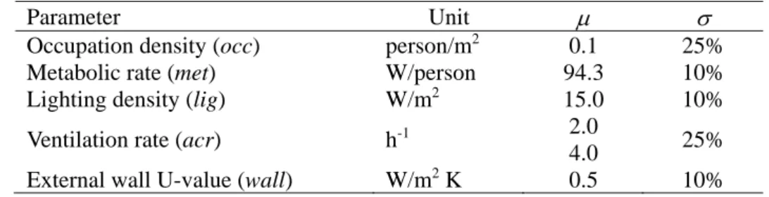
buildings energy simulation, the first step was choosing the input parameters. On the one hand, a large number of parameters would compromise the time-efficiency of the procedure and on the other, it is desirable that the most uncertain and potentially most influential parameters should be considered. Thus, 5 parameters were selected: occupation density, metabolic rate, lighting density, ventilation rate and external wall thermal resistance. For all it was assumed a normal distribution with the mean () and standard deviation () values presented in Table 1. Particular attention should be paid to the ventilation since several in situ measurements revealed that air change rates tend to be much lower than the ones predicted at design stage (Almeida, 2012). For that reason two mean values were considered for the air change rate.

TABLE 1. Normal distribution parameters

Parameter Unit  

Occupation density (occ) person/m2 0.1 25%

Metabolic rate (met) W/person 94.3 10%

Lighting density (lig) W/m2 15.0 10%

Ventilation rate (acr) h-1 2.0

4.0 25%

External wall U-value (wall) W/m2 K 0.5 10%

2.2 Number of samples and output

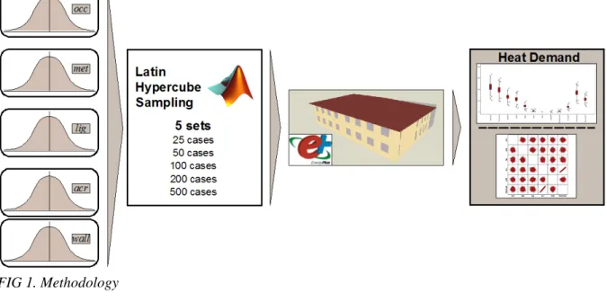
Five sets of the parameters, with different dimension, were computed in order to evaluate the convergence of the results. These combinations of parameters were obtained by using Latin Hypercube Sampling method, which is a stratified sampling method and can produce more stable

analysis results than random sampling. The MatLab algorithm lhsnorm was employed. Therefore, Monte Carlo simulations were performed for 25, 50, 100, 200 and 500 cases. The software chosen for the simulation was Energy Plus. This software is particularly adequate for the implementation of this methodology since its input files are text-based and, consequently, it was possible to automate the procedure of writing EnergyPlus models by means of an Excel VBA code. 1750 models were created and simulated.

The building simulation output chosen was the heat energy demand (Eannual), both monthly and annual. Figure 1 illustrates the procedure.

FIG 1. Methodology

2.3 Case study

The case study is a typical two storey Portuguese school building, dated from the 90’s, and this project of simple rectangular schools was repeated throughout the country. The building model was created with DesignBuilder.

Four types of zones were considered, each with specific metabolic rates, occupation density and schedules: classroom (545 m2_{), circulation (212 m}2_{), storage (130 m}2_{) and toilet (63 m}2_{). For the}

classroom zone was defined a metabolic rate of 94 W/person with an occupation density of 0.40 people/m2.

An in situ complete survey was carried in order to characterize the most relevant construction

elements properties. The school original walls and roof have no insulation and the windows are single glazed. Blinds with medium reflectivity slats were considered as shading devices, with operation by solar radiation control with a set point of 120 W/m2.

Ventilation is natural and the heat systems are hot water radiators, with a temperature set-point of 20ºC, which is in conformity with the Portuguese regulation.

The simulations were performed on an annual base, with hourly outputs, and considering 10 time steps per hour.

3. Results

Two kinds of analysis were performed: a convergence analysis and a sensitivity analysis of the results. The sensitivity analysis produced a large amount of results since it was performed for monthly and

annual heat demand. However, the scope of this paper is just to explore the opportunities and difficulties of the methodology on the uncertainty evaluation of the input parameters. For that some demonstrative examples were chosen.

3.1 Convergence analysis

The study started with the base case simulation. This case corresponds to the scenario where the mean value is assumed for all the parameters (Table 1).

The five sets of simulations were then performed and the annual heat demand computed. The mean value was calculated, compared with the base case and the corresponding error was determined by the following equation:

 

Where

E

0 annual

E heat demand obtained with base case (kWh/(m2.year))

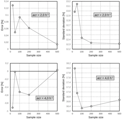
Standard deviation convergence was also analysed. Figure 2 shows the plot of the results.

0 0,02 0,04 0,06 0,08 0,1 0,12 0,14 0 100 200 300 400 500 E rro r [ % ] Sample size acr = 2,0 h-1 12,2 12,3 12,4 12,5 12,6 12,7 12,8 12,9 13,0 13,1 13,2 0 100 200 300 400 500 Sta ndar d d e vi ation [% ] Sample size acr = 2,0 h-1 -1 -0,8 -0,6 -0,4 -0,2 0 0,2 0 100 200 300 400 500 Err o r [% ] Sample size acr = 4,0 h-1 16,2 16,4 16,6 16,8 17,0 17,2 17,4 17,6 17,8 18,0 18,2 0 100 200 300 400 500 Standard devi a tion [%] Sample size acr = 4,0 h-1

FIG 2. Convergence analysis of the annual heat demand

The most important finding of this analysis is that all the sets performed very well. Even for the set of 25 cases an error below 1% was observed. However, it is important to refer that this conclusion is only valid for this particular problem. As stated before, several studies revealed that the sample size is

important for the overall accuracy of the method and can be responsible for very significant errors, particularly when a large number of inputs and outputs are analysed.

For the scenario of acr = 2.0 h-1 the best performance was achieved with the largest set (500 cases); for acr = 4.0 h-1 the best performing set was the one with 50 cases, followed by the one with 500 cases. Regarding the standard deviation, no convergence was found. However, differences between the sets are relatively small.

3.2 Sensitivity analysis

3.2.1 Monthly analysis

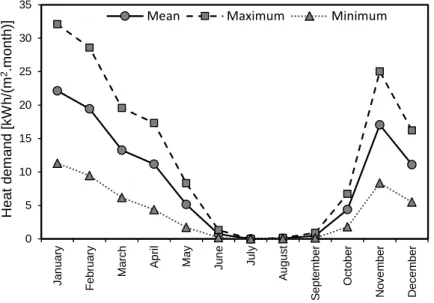
Figure 3 shows the mean, maximum and minimum monthly heat demand, obtained in the scenario of acr = 2.0 h-1 _{and a set of 500 cases.}

0 5 10 15 20 25 30 35 Jan uary F ebr uary M arch Ap ri l Ma y Jun e Ju ly Au g u s t S e pt em be r Oc to be r No v e m ber De c e m ber H eat de m and [k W h /(m 2.m onth

)] Mean Maximum Minimum

FIG 3. Monthly analysis

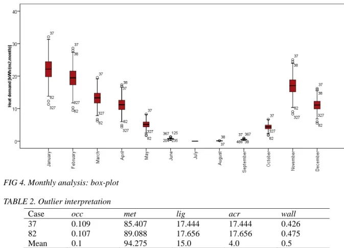
Another way to statistically analyse the distribution of these results is using the box-plot

representation, where the outliers of the sample can be observed. Outliers should be investigated carefully. Often they contain valuable information about the process under investigation. This form of representation (Figure 4) allows to easily identify situations of abnormally high or low heat demand, and if one checks the input values of the parameters for those cases, the relative importance of each parameter can be assessed. As an example, Table 2 includes the parameters input values of case 37 and 82, the first corresponds to a situation of high energy demand and the second of low demand.

Results indicate that air change rate plays a vital role in the result. The situation is confirmed by the correlation analysis presented in section 3.2.2.

FIG 4. Monthly analysis: box-plot TABLE 2. Outlier interpretation

Case occ met lig acr wall

37 0.109 85.407 17.444 17.444 0.426 82 0.107 89.088 17.656 17.656 0.475

Mean 0.1 94.275 15.0 4.0 0.5

3.2.2 Annual analysis

Annual heat demand was also evaluated. The histogram of the normalized heat demand is illustrated in Figure 5 and Table 3 summarizes the results. As in the case of the monthly analysis, the example refers to the same data (acr = 2.0 h-1; 500 cases).

0% 20% 40% 60% 80% 100% 0% 4% 8% 12% 16% 20% 40 60 80 100 120 140 160 C u mu la tiv e f req uen cy [% ] F req uen cy [% ] Heat demand [kWh/(m2_.year)] Frequency Cumulative

FIG 5. Annual distribution

TABLE 3. Statistical indicators

 104.9

 17.5

Maximum 156.2 Minimum 49.0 Coef. of variation 0.17

As it was expected a normal distribution of the results was obtained. The annual heat demand derived from the deterministic analysis (Table 1 input values for the five parameters) was also

104.9 kWh/(m2.year). However, if one considers the stochastic nature of the input parameters the available information increases. For the example under study, the Monte Carlo simulation reveal that in 68% of the scenarios the heat demand is between 87.4 and 122.4 kWh/(m2.year) (± ). Though, if one imposes a target of 90% probability an heat demand of 127.8 kWh/(m2.year) should be

considered. This kind of conclusions exposes the importance of stochastic analysis to technically support the decision-maker.

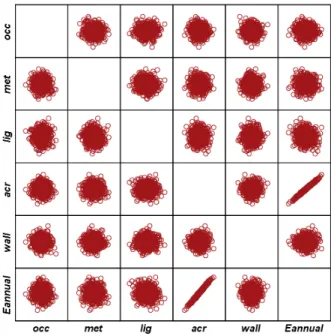
When one seeks to evaluate the influence of the uncertainty of the input data and in which manner they influence the result, giving the designer information about the relative sensitivity of the

parameters, an interesting and simple method is a graphical sensitivity analysis (Burhenne 2010). Each parameter and its corresponding result (e.g. occ1, Eannual1; …; occn, Eannual n) is plotted in a scatter

plot. Figure 6 shows a matrix of scatter plots for the 5 input parameters and the correspondent heat demand (acr = 2.0 h-1; 500 cases).

It can be seen that the annual heat demand of the building (Eannual) is very sensitive to air change rate (acr). Furthermore, an almost linear dependency between the parameter and the output can be observed. This result was confirmed by a correlation analysis between the input and output parameters whose results can be found in Table 4. A specific parameter can therefore arise as the only one relevant for the problem, alerting designers for the need of measures that increase robustness of, in this case, acr control during the school’s operation.

FIG 6. Scatter plot matrix for sensitivity analysis TABLE 4. Correlation analysis

occ met lig acr wall Eannual

occ met -0.06 lig 0.03 -0.07 acr -0.07 -0.04 -0.02 wall

-0.06

-0.08

It is important to refer that all the considerations exposed here for the scenario of acr = 2.0 h-1 _{and 500}

4. Conclusions

Buildings energy performance is nowadays a motive of concern for all European governments. In developed countries, buildings are responsible for a significant share of the total energy consumption and increasing in recent decades mainly due to the users growing comfort demands. In this context all the measures to improve the energy efficiency of buildings are welcome. Building simulation is an essential tool in building energy optimization. However, its use should be prepared carefully since only realist input data would lead to valuable outputs. Therefore, the stochastic nature of input data should be taken into account and uncertainty analysis should be performed.

This paper proposes a probabilistic approach to the evaluation of the uncertainty of input data in a school building energy simulation. Monte Carlo simulation is performed considering uncertainty in five input parameters. Building heat demand is the output.

The study included a convergence analysis of the results and a sensitivity analysis. Convergence analysis exposed that, for this particular situation, a small number of cases (25) are enough to obtain an error below 1%. Sensitivity analysis revealed that air change rate was the most important input in school buildings energy simulation. In fact, a linear dependency between air change rate and the annual energy demand of the building was found. A stochastic database is the final piece missing, after which this methodology can actually be applicable in practice.

References

Almeida R. & Freitas V.P., 2010. Hygrothermal Performance of Portuguese Classrooms: measurement and computer simulation. In: Proceedings of 1st Central European Symposium on Building Physics. Cracow, Poland 13-15 September 2010.

Burhenne S., Tsvetkova O., Jacob D., Henze G.P. & Wagner A. 2013. Uncertainty quantification for combined building performance and cost-benefit analyses. Building and Environment, 62, pp.143-154.

Burhenne S., Jacob D. & Henze G.P. 2010. Uncertainty analysis in building simulation with Monte Carlo techniques. In: Proceedings of Fourth National Conference of IBPSA-USA. New York City, USA 11-13 August 2010.

Hopfe C.J. & Hensen J.L.M. 2011. Uncertainty analysis in building performance simulation for design support. Energy and Buildings, 43, pp.2798-2805.

Macdonald I.A. 2009. Comparison of sampling techniques on the performance of Monte-Carlo based Sensitivity Analysis. In: Proceedings of Building Simulation 2009. Glasgow, Scotland 27-30 July 2009.

Rodríguez G.C., Andrés A.C., Munoz F.D., López J.M.C. & Zhang Y. 2013. Uncertainties and sensitivity analysis in building energy simulation using macroparameters. Energy and Buildings, 67, pp.79-87.