EAGLeNet - A Deep Multi-Task Learning CNN for Emotion, Age and Gender Recognition

(1)

EAGLENET – A DEEP MULTI-TASK LEARNING CNN FOR EMOTION,

AGE AND GENDER RECOGNITION

João Santos Crispiniano Vieira

Dissertation

Master in Data Analytics

Supervised by

Professor Doutor João Manuel Portela da Gama Doutor Brais Cancela Barizo

(2)

(3)

iii

Abstract

Facial analysis systems have become increasingly relevant to a growing number of applications. Since the recent advent of Deep Learning, particularly Convolutional Neural Networks, facial analysis tasks have been a trendy topic, as developed models are consistently breaking accuracy records on various tasks, many breaking the human-level barrier.

Accurate systems have been proposed for the tasks of emotion recognition, age estimation and gender recognition on face images, often at the expense of heavy models that require much processing power and time. The present work focuses on a solution for the three tasks deploying an efficient and fast system. To achieve this, various models derived from the same fundamental architecture were developed and compared, which perform the three tasks simultaneously on a single Convolutional Neural Network, through the use of a Multi-task learning approach.

The final models are efficient and fast, achieving successful results comparable to the Single-task models, supporting the Multi-task Learning approach.

Keywords: Facial analysis, Deep Learning; Convolutional Neural Networks; Multi-task Learning.

(4)

iv

Resumo

Os sistemas de análise facial têm vindo a ganhar relevância num número crescente de aplicações. Com o advento recente do Deep Learning, particularmente das Convolutional Neural Networks, as tarefas de análise facial têm-se tornado um tópico de interesse geral, muitas ultrapassando a performance do humano.

Sistemas precisos têm sido propostos para as tarefas de reconhecimento de emoção, estimação de idade e reconhecimento de género em imagens faciais, muitas vezes recorrendo a modelos pesados que requerem forte poder e tempo de processamento. O presente estudo foca-se em desenvolver uma solução rápida e eficiente para as três tarefas. Para o alcançar, vários modelos derivados da mesma arquitectura base foram desenvolvidos e comparados, realizando as três tarefas numa única Convolutional Neural Network. Para isso foi usada uma abordagem de aprendizagem Multi-task.

Os modelos obtidos são eficientes e rápidos, alcançando bons resultados, comparáveis aos dos modelos Single-task, assim suportando a abordagem Multi-task.

Palavras-chave: Análise facial, Deep Learning; Convolutional Neural Networks; Aprendizagem Multi-task.

(5)

v

2.1.3. Advances in CNNs ... 11 2.1.3.1. Convolution layer ...11 2.1.3.2. Pooling layer ...13 2.1.3.3. Activation function ...13 2.1.3.4. Regularization ...14 2.1.3.5. Optimization ...14 2.1.3.6. Structure...15 2.2. FACIAL ANALYSIS ... 18 2.2.1. Gender Recognition ... 18 2.2.2. Age Estimation ... 18 2.2.3. Emotion Recognition ... 19

2.3. MULTI-TASK LEARNING ARCHITECTURES ... 20

2.3.1. Deeply supervised MTL architecture ... 21

2.3.2. Parallel MTL architecture ... 23

2.4. DAGER – A COMMERCIAL APPROACH ... 24

CHAPTER 3 – METHODOLOGY ... 26

(6)

vi 3.1.1. Emotion recognition... 26 3.1.2. Age estimation ... 27 3.1.3. Gender recognition ... 28 3.2. DATABASES ... 29 3.2.1. Image Pre-processing ... 29 3.3. MODEL DESIGN ... 31

3.3.1. Baseline Network Architecture ... 32

3.3.2. Training procedure ... 34

3.3.2.1 Single-task Training...35

Architectures ...35

Model training – parameters, procedures and data handling ...37

3.3.2.1. Multi-task Training ...38

Architectures ...38

Model training – parameters, procedures and data handling ...41

3.4. SOFTWARE ... 42

CHAPTER 4 – RESULTS AND EVALUATION ... 43

4.1. SINGLE-TASK MODELS ... 43 4.1.1. Emotion Recognition ... 43 4.1.1.1. Class Unweighted ...44 Training phase ...44 Testing phase ...45 4.1.1.2. Class weighted...46 Training phase ...46 Testing phase ...47 4.1.2. Age Estimation ... 48 Training phase ...48 Testing phase ...49 4.1.3. Gender Recognition ... 50 4.1.3.1. Class unweighted ...50 Training phase ...50 Testing phase ...51 4.1.3.2. Class weighted...52 Training phase ...52 Testing phase ...53

(7)

vii 4.2. MULTI-TASK MODELS ... 54 4.2.1. Triple-Module Sharing (v1) ... 55 Training phase ...55 Testing phase ...57 4.2.2. Dual-Module Sharing (v2) ... 60 Training phase ...60 Testing phase ...62 4.2.3. Single-Module Sharing (v3) ... 65 Training phase ...65 Testing phase ...67 4.2.4. Zero-Module Sharing (v4) ... 69 Training phase ...69 Testing phase ...72 4.3. COMPARISONS... 74

4.3.1. Emotion task model comparison ... 74

4.3.1. Age task model comparison ... 76

4.3.1. Gender task model comparison ... 77

4.3.1. Global model comparison ... 79

5. CONCLUSIONS AND FINAL THOUGHTS ... 81

(8)

viii

List of Tables

Table 1 – Emotion dataset class distribution ... 29

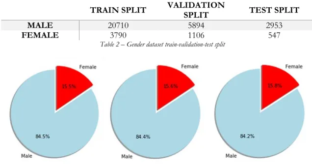
Table 2 – Gender dataset train-validation-test split ... 30

Table 3 - Emotion dataset train-validation-test split ... 30

Table 4 - Emotion training class weights ... 38

Table 5 - Gender training class weights ... 38

Table 6 – Class metrics ... 45

Table 7 – Model metrics ... 46

Table 14 – Emotion class metrics ... 58

Table 15 – Emotion metrics ... 58

Table 16 – Gender class metrics ... 59

Table 17 – Gender metrics ... 60

Table 30 – Emotion class model comparison ... 75

(9)

ix

Table 32 – Age model comparison ... 77 Table 33 – Gender class model comparison ... 78 Table 34 – Gender model comparison ... 79

(10)

x

List of Figures

Figure 1 - Traditional pattern recognition (LeCun et al., 1998) ... 6

Figure 2 - General CNN architecture (Guo et al., 2016) ... 7

Figure 3 - Mathematical model of a neuron (Cadène et al., 2016) ...10

Figure 4 - Residual Connection (He et al., 2016) ...16

Figure 5 – Global Average Pooling (Cook, 2017) ...17

Figure 6 - Deeply supersized MTL architecture (Ranjan et al.,2017) ...23

Figure 7 - Parallel MTL architecture (Xing et al., 2017) ...24

Figure 8 - DAGER framework (Dehghan et al., 2017) ...25

Figure 9 - Gender dataset train-validation-test split ...30

Figure 10 – Emotion dataset train-validation-test split ...30

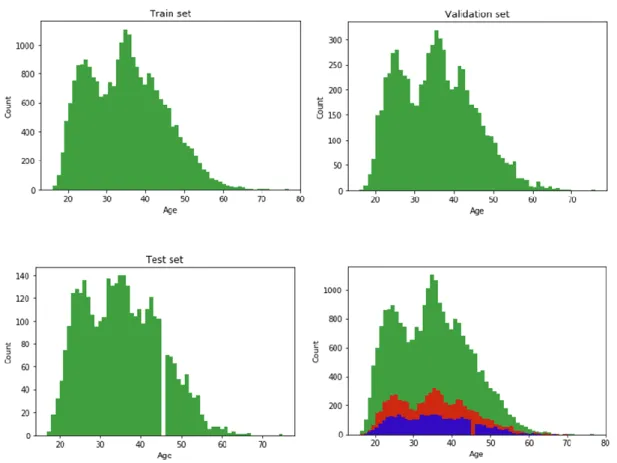
Figure 11 - Age Distribution for the training set, validation set, test set and the merged sets ...31

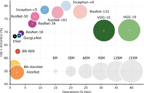
Figure 12 - Framework Comparison (Operations per Accuracy) (Canziani et al., 2017) ...32

Figure 13 – Baseline Architecture ...34

Figure 14 - Emotion Recognition Model ...35

Figure 15 - Age Estimation Model ...36

Figure 16 - Gender Recognition Model ...36

Figure 17 - V1 model architecture ...39

Figure 21 - Training and validation loss (real and smoothed) ...44

Figure 22 - Training and validation metrics (real and smoothed) ...44

Figure 23 – Confusion matrix ...45

Figure 26 - Confusion matrix ...47

Figure 27- Training and validation loss (real and smoothed) ...49

Figure 29 – MAE per age results...50

(11)

xi

Figure 36 - Emotion training and validation loss (real and smoothed) ...55

Figure 37 - Emotion training and validation metrics (real and smoothed) ...56

Figure 38 - Age training and validation loss (real and smoothed) ...56

Figure 39 - Age training and validation metrics (real and smoothed) ...56

Figure 40 - Gender training and validation loss (real and smoothed) ...56

Figure 41 - Gender training and validation metrics (real and smoothed) ...57

Figure 42 - Aggregated gender and age training and validation loss (real and smoothed) ...57

Figure 43 - Total training and validation loss (real and smoothed) ...57

Figure 44 – Emotion confusion matrix...58

Figure 46 – Gender confusion matrix ...59

Figure 48 - Emotion training and validation metrics (real and smoothed) ...61

Figure 55 - Emotion confusion matrix ...63

Figure 56 – Mae per age results ...64

Figure 58 – Emotion training and validation loss (real and smoothed)...65

Figure 59 – Emotion training and validation metrics (real and smoothed) ...65

Figure 60 – Age training and validation loss (real and smoothed) ...66

Figure 61 – Age training and validation metrics (real and smoothed) ...66

Figure 62 – Gender training and validation loss (real and smoothed) ...66

Figure 63 – Gender training and validation metrics (real and smoothed) ...66

Figure 64 – Aggregated gender and age training and validation loss (real and smoothed) ...67

Figure 65 – Total training and validation loss (real and smoothed) ...67

Figure 66 – Emotion confusion matrix...68

Figure 67 - MAE per age result ...68

(12)

xii

Figure 77 - Emotion confusion matrix ...72

(13)

1

Chapter 1 – Introduction

A change of paradigm is currently underway. Computers have been consistently surpassing humans in many tasks of the day-to-day life in the past decades, with us relying more and more on them. If a bank’s database servers would for some reason shutdown and wipe out all of its information, the world economy could collapse. We are in the age of information, and that information is increasingly being collected and stored by machines. Machine Learning uses this information to learn patterns. It can be used to predict the weather, to help on credit approval, or to recommend a visit to the doctor if an irregular heartbeat is detected.

But this change of paradigm is currently occurring in a specific subfield of computer science – computer vision, fueled by the advent of Deep Learning and Convolutional Neural Networks. Over the last decade, the rate of image uploads to the internet has been increasing exponentially. Motivated by this and the fact that high computing power is becoming increasingly accessible to the common user, more and more research is being done on computer vision. Problems that were once considered impossible to study due to lack of data or computing power are being attempted now (Ekmekji, 2016). Cars can drive themselves nowadays, detecting pedestrians and predicting/avoiding accidents. Despite self-driving cars being a hot-topic today, there is perhaps one even hotter – facial analysis.

Facial analysis comprehends several tasks, which can be used for several purposes. There are models for the task of face detection, pose estimation, age estimation, face recognition, smile detection, gender recognition, and so on. In many cases, machine-estimation has been consistently breaking the human level, achieving outstanding results. There is a sense of urgency in the quest to investigate and develop the best model, fueled by Artificial Intelligence competitions and the tech business world. These systems can be applied to security systems, person identification, human-computer interaction platforms, marketing, etc.

We are getting closer, step by step, to become fully connected to technology, which can now lea and estimate our needs and characteristics. Facial analysis plays a key role in this scenario, as a significant part of human communication is nonverbal.

(14)

2

1.1. Problem Definition

The present dissertation seeks to propose a new framework of a single Convolutional Neural Network for the simultaneous tasks of age estimation, gender recognition and emotion recognition on face images. With the purpose of being able to perform all three tasks in a single network, a multi-task learning architecture is used, jointly learning the various tasks.

Using a baseline Convolutional Neural Network architecture, modifications are made to incorporate the three tasks, changes are made to the baseline architecture processes and layers, and various loss functions are considered. This has the objective of attaining an efficient and fast Multi-task working model. Various models are created with different shared layers across tasks, evaluating and comparing them on a test set. The final models should be able to provide insights on a face image concerning the age of the individual outputted in a real valued variable, the emotion of the individual outputted in one of seven classes (anger, disgust, happiness, fear, surprise, sadness and neutrality), and the gender of the individual outputted in one of two classes (male or female).

1.2. Motivation

Facial analysis systems can ultimately change the way we live. Allied to Artificial Intelligence, it can provide personal assistance in every aspect of life. It can estimate our mood upon waking and, connecting it to our habits, age and other factors, provide the perfect meal for the moment, the best music to accompany that meal, and the perfect outfit, linked to the weather prediction. Likewise, upon entering a clothing store, it can automatically suggest the best piece of clothing for you, according to your age and gender, and send to your smartphone a picture of you virtually dressed in such suggestions.

Machines will be capable of taking care of the uninteresting part of life, end-to-end. Supported by computer vision and facial analysis, the full connection and understanding of humans will soon happen. In fact, many state-of-the-art models have already outpaced human recognition in many facial analysis tasks.

Deep Learning and Convolutional Neural Networks are a hot-topic in the field of Machine Learning. Many breakthroughs are being reached every other day. Being a part of that is what motivates me to develop this work. As far as it is possible to determine, a Deep

(15)

3

Multi-Task Learning Convolutional Neural Network for Emotion, Age and Gender Recognition is still to be developed, and such an endeavor would certainly constitute a valuable contribution to Machine Learning.

1.3. Structure of the dissertation

The present dissertation is organized as follows: an introductory chapter, a literature review, the methodology approach, the results and evaluation and the concluding thoughts.

In the first chapter, the topic of the dissertation is introduced, as well as the problem description. The main motivations to the development of the study are then presented, followed by a brief description of the structure of the dissertation.

The second chapter covers the literature review, where firstly a description of Deep Learning and Convolutional Neural Networks is presented, followed by a review on facial analysis and the tasks proposed as the problem in this dissertation.

In the third chapter the methodology is described, explaining the task formulation and detailing the intended models. The databases for training, model design and training, testing procedure, and finally the used software are also explained.

A fourth chapter presents the results and evaluation of the developed models, each with interpretations over the training and testing phase, finalizing with a thorough model comparison section.

The fifth and final chapter outlines the final thoughts and conclusions on the developed work.

(16)

4

Chapter 2 – Literature Review

The present chapter introduces the concepts and descriptions relevant to the present study. Firstly, the definition of Deep Learning is introduced, followed by a more exhaustive description of Convolution Neural Networks, an application of such method which is the baseline concept of the present dissertation. Secondly, the topic of facial analysis is reviewed, focusing on the main tasks to be developed in the course of the study. The third section introduces the multi-task learning concept, where some examples are drawn to better expose the topic. Finally, a specific commercial related work is mentioned.

2.1. Deep Learning and CNNs

In this section, an introduction to Deep Learning is presented, briefly describing its evolution. Secondly, in a more exhaustive way, Convolutional Neural Networks are reviewed, defining and explaining each layer, elucidating the main differences between a CNN and regular Neural Network. Finally, the main advances achieved in each layer and process are outlined, with special emphasis on the ones used throughout this work.

2.1.1. Deep Learning: definition and evolution

There is a subfield of Machine Learning which aims to discover multiple levels of distributed representations – such field is called Deep Learning. Deep Learning relies on hierarchical architectures to learn high-level abstractions in data (Y. Guo et al., 2016). Various traditional machine learning tasks have been improved through the use of deep learning algorithms, such as semantic parsing (e.g. Bordes et al., 2012), transfer learning (e.g. Ciresan et al., 2012b), natural language processing (e.g. Mikolov et al., 2013) and computer vision (e.g. Ciresan et al., 2012a; Krizhevsky et al., 2012) among others.

Traditional Machine Learning techniques are limited in tasks such as object recognition in images, mainly because of their capacity for processing natural data – data in its raw form – hence the need to develop and use Deep Learning, a more advanced technique in representation learning (LeCun et al., 2015).

Deep Learning is a class of Artificial Neural Networks (NNs). Standard NNs, or Shallow NNs, have been around at least since the 1960s. They consist of many simple connected

(17)

5

neurons, which can be viewed as simple processors, where each one produces an arrangement of real-valued activations. They are divided in two sections: the input neurons, activated through the perception of the environment through sensors, and other neurons, activated through weighted connections to previously activated neurons. The environment might be influenced by actions deployed by some neurons. Shallow NNs and Deep NNs are distinguished by the depth of these chains of connected neurons, which are chains of possibly learnable causal links between action and effects (Schmidhuber, 2015).

Deep Learning became feasible in some areas during the 1990s and saw many improvements during the 1990s and 2000s. In the 21st century came the boom of Deep Learning, attracting wide-spread attention, due to the development of models that outperformed alternative machine learning methods, and the fact that supervised deep NNs have won various international machine learning competitions since 2009, even achieving better results that human visual pattern recognition in some domains (Schmidhuber, 2015). The boom in the development of DL methods is due to three main reasons: increased chip processing capacity, lowered cost of computing hardware, and the considerable achievements mentioned previously (Y. Guo et al., 2016).

Early supervised Neural Networks were variants of linear regression methods, dating back to the early 1800s in the work of Gauss. But simple Artificial Neural Networks architectures were firstly developed in the 1940s, and in the following decades the use of supervised learning techniques were introduced to these architectures. During the 1960s, the discovery of simple and complex cells in the cat’s visual cortex later inspired deep NN architectures used in award-winning models. Throughout this decade, NNs trained by the GMDH method – Group Method of Data Handling – were the first kind of Deep Learning systems. In 1979 Fukushima introduced the Neocognitron, the first truly deep NN, a convolutional NN. The first efficient application of backpropagation in NNs was described in 1981 (Schmidhuber, 2015).

2.1.2. Convolutional Neural Networks

Having presented the definition of Deep Learning, Convolutional Neural Networks (CNNs) are now addressed. CNNs are shown to outperform all the other techniques in image pattern recognition tasks, exemplified in Figure 1. They are one of the best Deep

(18)

6

Learning techniques with a robust multiple layer training (LeCun et al., 1998). Proving to be highly effective, they are the most commonly used in computer vision and speech recognition problems (Y. Guo et al., 2016).

Figure 1 - Traditional pattern recognition (LeCun et al., 1998)

Multilayer networks’ ability to learn complex, high dimensional, nonlinear mappings through large datasets makes them candidates for image recognition tasks. This can be done with regular fully connected feedforward networks with some success, but there are mainly two problems (LeCun et al., 1998).

Firstly, images are often large, with several thousands or millions of pixels, which would work as variables, and a fully connected first layer with, for example, one hundred hidden units in the first layer would comprehend several tens of thousands of weights. Several parameters increase the capacity of the system, requiring a larger training set. Furthermore, the toll taken on memory from storing so many weights may exclude some hardware implementations. Perhaps the greater problem of unstructured nets for image or speech applications is the fact that the feeding of the input layer, the signals, such as images, must be approximately size normalized and centered (LeCun et al., 1998). This can be automatically achieved in CNNs, as will be described later.

Secondly, there is the problem concerning the topology of the input: it is entirely ignored – the outcome of the training is not affected by the input order of the variables. This poses a problem because images have a strong two-dimensional local structure, being that pixels spatially close are highly correlated. CNNs perform better relative to this problem since they search and extract local features restricting the receptive fields of hidden units locally (LeCun et al., 1998), as will be later described.

(19)

7

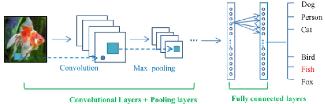
A typical CNN (Fig. 2) comprehends three main neural layers: convolutional layers, pooling layers, and fully connected layers. Usually, the convolutional layers alternate with pooling layers, followed by some fully connected ones at the end of the network. All of them perform distinct roles. There are two training stages of the network, a forward stage and a backward stage. During the first, the effort is on the representation of the input image with the current parameters, weights and biases, in each layer, comparing the predicted to the ground truth labels for the computation of the loss cost. Secondly, and using this loss cost, the network’s backward stage computes the gradients of each parameter with chain rules to update all the parameters of the network, preparing it for the next forward computation. With enough iterations of the two stages, the network learning can be stopped (Y. Guo et al., 2016).

In the following section the description of each layer is presented.

Figure 2 - General CNN architecture (Guo et al., 2016)

2.1.2.1. Layers

Convolution layers

The purpose of convolution layers is to build feature maps by convolving the whole image, as well as the intermediate feature maps, with the use of various kernels (Y. Guo et al., 2016). In image processing, a kernel is a two-dimensional matrix of numbers used to compute new matrices by performing some calculations between the kernel and the input picture or feature map. The input image is nothing but a matrix as well, such as in an 8-bit RGB image, for example, in which each pixel (each cell of the matrix) is represented by three numbers with a value ranging from 0 to 255 (red, green and blue information). There are multiple kernels for various tasks in image processing, such as blurring and edge detection (Cope, 2017).

(20)

8

In an image, close pixels exhibit many spatial relationships among them. The location of such neighboring pixels within the image should not affect these spatial relationships. A convolution layer is instructed with a set of filters (or kernels), which are analogous to templates. A number of these filters are convolved with the input image to generate feature maps, by matching the learned filters to every possible patch of the image. If the filter has a high correlation with a region of the input image, the resulting feature map will have a strong response in the location of such region (Zeiler, 2014).

So, the convolutional layer focuses on learning feature representations of the inputs. One convolution layer is composed of several convolution kernels to compute different feature maps. A new feature map is obtained by first convolving the input image or feature map with a learned kernel and then applying a nonlinear activation function, specified later in the study, on the convolved results. On a newly obtained feature map, each neuron is connected to a set of neighboring neurons in the previous layer, called the receptive field of this neuron in the previous layer. During the generation of each feature map, all the spatial locations of the input share the same kernel. The complete set of feature maps generated at each convolution layer is obtained through the use of several different kernels (Gu et al., 2017).

A spatial convolution is defined by (1) the number of filters, as the number of output channels, (2) by the properties of such filters, as the number of input channels and its width and height, (3) and the properties of the convolution process, like the padding or stride size (Cadène et al., 2016).

The use of convolution layers provides three main advantages: (1) for the same feature map, there is a mechanism for weight sharing which decreases the number of parameters; (2) correlations among neighboring pixels is learnt through local connectivity; (3) equivariance - the location of the object is not important, there is an invariance towards it (Zeiler, 2014).

Pooling layers

Pooling layers are used in CNNs to provide invariance in cases where the input images have just minute differences, and to reduce the dimensionality of the feature maps. A pooling function is used over a region of pixels. One of the most common functions is Max pooling, where, during backpropagation, the gradient is placed in a single location, making this function one of the preferred ones as it dodges cancellation of negative elements and prevents blurring of the activations and gradients throughout the network (Cadène et al.,

(21)

9

2016). Another common pooling strategy is average pooling, but max pooling is capable of achieving faster convergence of the network, improve the generalization requiring less training examples selecting better invariant features (Scherer et al., 2010). Most of the recent CNN implementation nowadays utilize max-pooling (e.g. Ciresan et al., 2011; Krizhevsky et al., 2012).

A pooling layer usually follows a convolutional layer and has the ability to reduce the dimensions of feature maps and networks parameters. As previously stated, and similarly to convolutional layers, they are translation invariant, as their computations consider the neighboring pixels. This type of layer is the most extensively studied (Y. Guo et al., 2016). The three more relevant new approaches on the pooling method, aside from the common max-pooling and average-pooling: (1) the Stochastic pooling, which works similarly to standard max pooling, but tries to overcome a common problem of this method, which is overfitting to the training dataset (making it harder to generalize), by creating many copies of the input image each having small local deformations (Zeiler & Fergus, 2013); (2) the Spatial pyramid pooling, developed by He et al. (2015b), a solution to deal with different scales handling, sizes and aspect ratios, as the other methods require a fixed-sized input image, which can be applied to any CNN architecture replacing the last pooling layer (Liu et al., 2014); (3) the Def-pooling, which tries to deal with the deformation of visual patterns more efficiently than max-pooling (Ouyang et al., 2015). The various strategies can be used in combination in order to boost the CNN’s performance.

In sum, the aggregation function, the dimensions of the area where it is applied and the convolution’s properties are the elements that define the spatial pooling layer (Cadène et al., 2016).

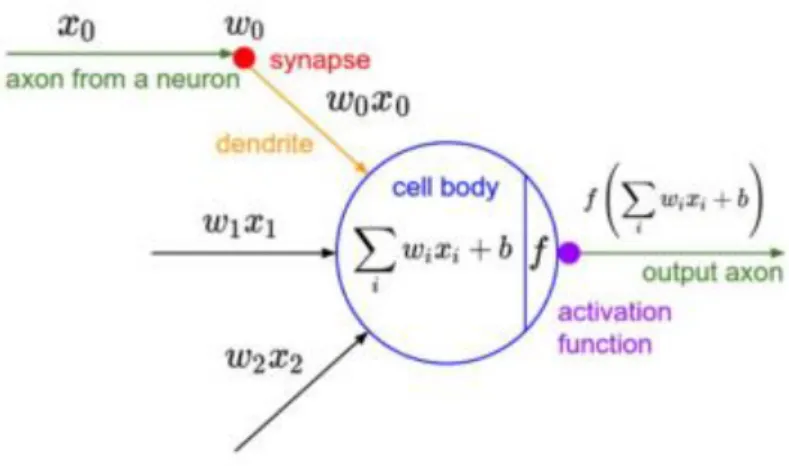
Fully Connected layers

The fully or linear connected layer motivation is the basic processing unit of the brain, the neuron (Fig. 3). It contains several neurons and can be mathematically seen as a function that applies a linear transformation on an input vector, and outputs another vector with another dimension, usually having a bias parameter. In each layer, every neuron is connected to the same input layer – hence fully connected - and outputs a signal (Cadène et al., 2016). CNNs high-level reasoning is performed in these layers. Every neuron in a fully connected layer is connected to all the feature maps in the previous layer. Usually the last layer of the

(22)

10

network is the loss layer, where the penalty of the deviation between predicted values and true ones is specified, during the training of the network. There are various loss functions available, and the choice of which to use relies on the type of problem. Softmax loss is the most commonly used, and it is applied on classification problems where the prediction is a single class between a set of mutually exclusive ones. Sigmoid cross-entropy loss is commonly used in classification tasks of 𝑁 independent classes with probability between zero and one. Euclidean loss is mostly used on regression problems with real-valued labels (Gomez et al., 2015). The CNN training process is a global optimization process: the best fitting set of parameters are obtained by trying to minimize the loss function (Gu et al., 2017). Thus, the last pooling layer in the network is usually followed by these layers of fully connected neurons, where the two-dimensional feature map is converted into a one-dimensional feature vector. These layers are the same as in traditional neural networks and hold 90% of the parameters of a CNN (Y. Guo et al., 2016). After the feed forwarding process, the resultant vector could be used for image classification category selection (e.g. Krizhevsky et al., 2012), or it can be used as a feature vector for follow-up processing (e.g. Girshick et al., 2014).

The fact that these layers hold so many parameters comes at the cost of large computational effort for training them. One way to deal with this is by removing the layers altogether, or by decreasing the connections between neurons with some method (Y. Guo et al., 2016). The GoogLeNet model handled this problem by switching these layers from fully connected to sparsely connected, maintaining the computational budget constant, using an Inception module (Szegedy et al., 2015), which is described in the next section.

(23)

11

Non-linear Activation Functions

The activation function is the identity function responsible for the output of real values. The ability for NNs to approximate any functions comes from the non-linear activation functions. In CNNs it is desirable to detect nonlinear features. There are three typical activation functions: the sigmoid, the hyperbolic tangent and the Rectified Linear Unit functions. The sigmoid function (1) takes as an input a real value and crushes it, with its output being between 0 and 1 – when the activation is at its limits, low or high, these regions gradient is almost zero, making the backpropagation stage fail at modifying the parameters of this layer and the preceding ones. The hyperbolic tangent function (2) works similarly to the sigmoid function but the output is between -1 and 1, and has the same problem. The rectified linear unit function or ReLU (3), developed by Nair & Hinton (2010), works differently as its transformation does not crush the input value. Aside from removing all the negative information from the previous layer, making it inadequate to some datasets, ReLU has become quite popular in the last years as it accelerates the convergence of stochastic gradient descent (compared to the previous functions) due to its form being linear and non-saturating. As the mathematical operations are simpler, compared to the other two functions, ReLU is a more reliable and efficient activation function (Cadène et al., 2016). In fact, research revealed that ReLU achieves better performances than those two functions (e.g. Maas et al., 2013).

In the following section the recent advances in some of the CNNs’ methods are outlined.

2.1.3. Advances in CNNs

Since the success of AlexNet in 2012, various improvements have been applied to CNNs, as noted by Gu et al. (2017). In the next paragraphs, the most relevant and recent methods of the different layers of CNNs are introduced, which were considered in the development of this study.

2.1.3.1. Convolution layer

In the convolutional layer, various methods have been suggested to enhance its representation ability, three of which are now outlined. The first (1) is the Network in Network (NIN), a method where the linear filter of the convolutional layer is replaced by a

(24)

12

small network – the original method proposed a multilayer perceptron convolution (mlpconv) – making it possible to better approximate more abstract representations (Lin et al., 2014). The second (2) is the Depthwise Separable Convolution, a method developed by Laurent Sifre while interning at Google Brain with the main purpose of improving the convergence speed and reduction in model size of the AlexNet. This method performs Depthwise convolutions followed by Pointwise convolutions over the input feature maps. The main advantage is the reduction of computation time and number of parameters. Instead of performing convolutions for each kernel over all the channels of the input feature map and summing them (like a traditional convolution) – where each kernel has the same number of channels as the input feature map – this method employs a different method. Firstly it performs Depthwise convolutions over each channel of the input feature maps – the kernel has only one channel – and then performs Pointwise convolutions over its output – which uses a kernel with size 1x1 and the number of channels of the output. Compared to a traditional convolution layer, a Depthwise Separable convolution has much less parameters as it performs much less multiplications for the same input and output size. It tends to output comparable results, with just a slight deterioration, but with a sizeable reduction of computation time (Chollet, 2017; Vanhoucke, 2014). Finally (3), the Inception Module, is a method where there is an application of flexible filter sizes to capture varied visual patterns of different sizes and approximation to the optimal sparse structure by the inception module, where one pooling and three types of convolution operations take place. This allows for larger CNNs, increasing the depth and the width, without increasing the computational cost. Compared to AlexNet’s 60 million parameters and ZFNet 75 million, the application of the inception module permits the reduction of the network’s parameters to 5 million (Szegedy et al., 2015). Such method, under the name GoogLeNet, obtained state-of-the-art results in the ImageNet 2014 challenge. The newest inception module CNN proposed by the same author, attempting to find a high-performance network considering the computation cost and inspired by the ResNet architecture (He et al., 2016), combines the inception architecture with shortcut connections. It is called the Inception-V4, and the use of such shortcut connections enables faster training regimens (Szegedy, Ioffe, et al., 2017).

(25)

13

2.1.3.2. Pooling layer

In the pooling layer, various methods have been proposed to enhance the provided invariance and lowered computation cost (by reducing the number of connections between convolutional layers through the reduction of the feature maps). Four of these methods are briefly outlined, which could be considered more relevant: (1) Lp Pooling, a method inspired by the biology of complex cells that can provide better generalization than max-pooling (Bruna et al., 2014); (2) Mixed Pooling, a combination of max-pooling and average-pooling that can provide better results than each of them, and can improve the overfitting problems (Yu et al., 2014); (3) Spectral Pooling, a form of pooling where the dimensionality reduction is achieved by cropping the representation of the input in frequency domain. This method can maintain more information than max-pooling for the same output dimensionality, avoiding its sharp reduction like other pooling strategies (Rippel et al., 2015). Finally, (4) Multi-scale Orderless Pooling, a method that tries to improve the invariance of CNNs without the loss of information. The extraction of deep features is done globally and also locally with different scales (Gong et al., 2014).

2.1.3.3. Activation function

Various activation functions have been experimented, as a proper implementation can significantly improve the performance of a CNN (Gu et al., 2017). Four of such activation functions are now delineated, all of which achieve successful results. The first, (1) Leaky ReLU is a derivative of ReLU that compresses the negative part, contrary to transforming it to zero, losing less information than ReLU (Maas et al., 2013). A similar function to LReLU, (2) Parametric ReLU, tries to adaptively learn the parameters of the rectifiers, improving accuracy, and the extra computational cost is negligible (He et al., 2015a). (3) Randomized ReLU, another derivative of Leaky ReLU, assigns the parameters of negative parts randomly sampling from a uniform distribution in training, and then fixing its values in testing. The author compared ReLU, LReLU, PReLU and RReLU on an image classification task and concluded that those with a non-zero slope in the negative part in rectified activation units (all of them except ReLU) improved the performance of such task (Xu et al., 2015). Finally, (4) ELU - Exponential Linear Unit, is also a derivative of ReLU where a saturation function is employed for the negative part. It can enable the deep neural networks to train faster and can lead to higher performances (Clevert et al., 2016).

(26)

14

2.1.3.4. Regularization

Regularization methods are used to reduce overfitting in deep CNNs. Of the various methods available, four are subsequently described, considered the most relevant. The first (1), Lp-norm Regularization, a method that alters the objective function (activation or loss) by adding a term that penalizes the model complexity, which can reduce overfitting through the addition of variance (Gu et al., 2017). The second (2), Dropout, proved to be effective in reducing overfitting. The authors applied it to the fully-connected layers, aiming to prevent the network from relying too much on specific neurons, allowing it to be accurate even without full information. (Lu et al., 2016). (3) SpatialDropout, a derivative of Dropout developed to further prevent overfitting which works particularly well if the training data size is small (Tompson et al., 2015). Finally, (4) DropConnect, a method inspired by Dropout that does not change the value of the outputs of the neurons, but instead modifies the weights between them (Wan et al., 2013).

2.1.3.5. Optimization

The loss function at the end of a CNN quantifies the quality of the network with a defined set of weights for the task at hand. The goal of the process of optimization is to find the best set of weights in order to minimize the loss function.

The most commonly used optimization method is the gradient descent. To find the best direction in the weight-space that would minimize the loss function by improving the weight vector, a random search algorithm would be impractical. Instead, one could follow the gradient of the loss function. The gradient of the loss function is a vector of numbers containing the derivatives for each dimension in the input space, the partial derivatives. Following the gradient makes it possible to search in the direction of the best set of parameters, guaranteeing the best possible result in an infinite amount of time. It is possible to compute the gradient either numerically, calculating the partial derivative of the loss function for each dimension by making a small change and noticing how much the function changed, or analytically, using Calculus to derive a direct formula for the gradient. Gradient Descent is the process of repeatedly evaluating the gradient and updating the parameters of the network, following its direction in a defined adaptative or not amount – learning rate – one of the hyperparameter settings in the training phase of a neural network (Karpathy, 2018).

(27)

15

There are several algorithms to optimize the gradient descent mechanisms, counteracting some challenges: difficulty choosing a proper learning rate, applying the same learning rate to all the parameter updates even when the features have very different frequencies, and finally the difficulty of avoiding getting trapped in saddle points - points where one dimension slopes up and another slopes down, usually surrounded by a plateau of the same error as the gradient is very small in all dimensions (Dauphin et al., 2014). (Ruder, 2017a). The Adaptive Moment Estimation – Adam – is a method that tries to work around these challenges. Combining the advantages of two popular methods, AdaGrad, which performs well with sparse gradients, and RMSProp, which performs well in on-line and non-stationary settings. Adam is forthright to implement, is computationally efficient, has minute memory requirements and performs well on problems with large datasets and large networks (many parameters) (Kingma & Ba, 2017).

2.1.3.6. Structure

In 2015 Microsoft Research introduced Deep residual networks, a kind of network that uses residual blocks. These networks achieved state-of-the-art results on ImageNet and COCO 2015 competitions, which comprehended image classification, object detection and semantic segmentation.

Network depth is of critical importance in neural networks architectures. In fact, it has been recently demonstrated a mathematical proof revealing the utility of having deeper networks rather than wider networks (Eldan & Shamir, 2016). Motivated by this insight, the residual learning framework was developed. By applying it, it is possible to train deeper networks, leading to improved performances. Residual networks are deeper than their non-residual equivalents, yet they use a similar number of parameters.

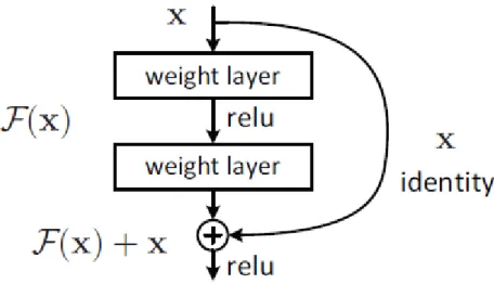
Increasing the depth of a regular network leads to a saturated accuracy, which eventually degrades. This degradation is not caused by overfitting, and increasing the number of layers to a capable deep model leads to higher training error. But considering a shallower architecture, there is a solution to a deeper counterpart (with more layers) model by construction: copying the layers from the shallower model, and the added layers are identity mapping. In this case, the deeper model should produce an error not greater than its shallower counterpart. So, the degradation problem is addressed through the use of a deep

(28)

16

residual learning framework, in which each few stacked layers fits a residual mapping (He et al., 2016). The basic framework can be seen in Figure 4.

Figure 4 - Residual Connection (He et al., 2016)

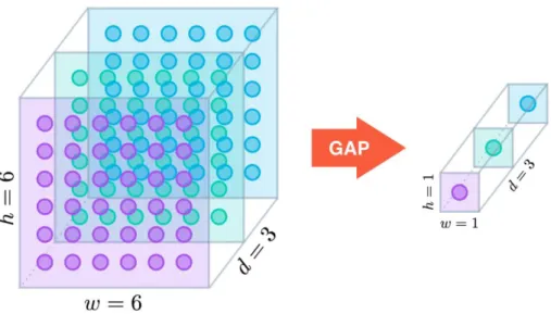
Another great advance in the CNN structure is the Global Average Pooling. Typically, a CNN architecture is a sequence of convolution layers followed by pooling layers, concluding in two or more densely connected layers, with the last one having a softmax activation function and a neuron for each class. These last fully connected layers usually contain most of the parameters of the network. This leads to overfitting to the training set, mitigated by the use of regularization methods and datasets as large as possible.

In recent years Global Average Pooling (GAP) was introduced to minimize overfitting by reducing the total number of parameters in the model. This fact has consequences like less computation required and faster models. Similar to max pooling layers, GAP layers are used to reduce the spatial dimensions of a 3D tensor. They take a tensor with size ℎ × 𝑤 × 𝑑 and reduce it to 1 × 1 × 𝑑, by averaging each feature map, ℎ × 𝑤, to a single number (Fig. 5). GAP can be seen as a structural regularizer, as it explicitly enforces each feature map to be directly connected to a category of the classification task (Lin et al., 2014).

(29)

17

Figure 5 – Global Average Pooling (Cook, 2017)

Another recently proposed mechanism accelerated the training of Deep Neural Networks by as much as fourteen times fewer training steps in a state-of-the-art image classification model, aside from allowing a significantly better accuracy margin. This development, Batch Normalization, works by reducing the internal covariance shift of each layer’s inputs. The distribution of each layer’s inputs changes as the parameters of the previous layer are updated during the training process: every time the optimization process occurs and updates the parameters of each layer. The changing input distribution is referred as Internal Covariate Shift. This is a problem as it slows down the training process by requiring lower training rates and careful parameter initialization. To counteract it, a mechanism of normalizing each layer’s inputs for each training mini-batch – fixating the means and variances of layer inputs - is performed. This process allows for higher learning rates, speeding up the training process, and it acts as regularizer, inducing some noise to each hidden layer, reducing overfitting and reducing the need to use other regularization methods such as Dropout and 𝐿2 weight

regularization (Ioffe & Szegedy, 2015).

Having provided a broad description of the CNN process and internal mechanisms, and outlined its most relevant and recent advances, it has been established that the Convolutional Neural Network is the state-of-the-art method in almost every subfield of computer vision. Hence, an overview of the three facial analysis’ tasks (based on this method?) is presented in the following section.

(30)

18

2.2. Facial Analysis

In recent years, the status quo of perception science has been challenged. For a long time, biological systems were the only ones with the ability of perception, as it was little understood in its inner workings. With the evolution of Deep Learning systems, however, neural networks are routinely outperforming humans in recognition and estimation tasks (VanRullen, 2017).

In the next three sections, a brief introduction to the tasks of emotion and gender recognition and age estimation through computer vision are outlined, with the most common or classic methods. In every task, evidence is presented to show that CNNs achieve the state-of-the-art results.

2.2.1. Gender Recognition

Recently, computer vision researchers have been giving increased attention to identifying demographic attributes, such as age and gender. These attributes are termed as soft biometrics and have applications in areas such as human-computer interaction, surveillance, biometrics, content-based retrieval, demographics collection and intelligent marketing. Gender recognition by humans achieve accuracies above 95% based only on face images, but it is still a challenging task for computer vision (Ng et al., 2015).

The early methods of gender recognition used many different classifiers to solve the problem, such as Neural Networks (e.g. Golomb et al., 1991), SVM (e.g. Moghaddam & Yang, 2002) and AdaBoost (e.g. Baluja & Rowley, 2007). Recently, the advances in CNN have outperformed every other method, making it the state-of-the-art in most benchmarks (Levi & Hassncer, 2015).

2.2.2. Age Estimation

The human age estimation process is not flawless. In fact, it is usually a more complex and challenging task than determining other facial information features, such as identity, expression and gender. Hence, developing automatic machine processes to do so, capable of equaling or even outperforming the human ability to estimate age became an attractive and challenging topic in recent years (Abousaleh et al., 2016).

(31)

19

Predicting the age from a face image has been a complex challenge in computer vision. There are many applications to this task, such as precision advertising, intelligent surveillance, face retrieval and recognition, etc. The variability of the images, the gender differences and other factors, impose subtle but relevant complexity to the age estimation task (Xing et al., 2017).

The classic age estimation methods usually perform two consecutive but independent procedures: given an input face image they start by performing a facial feature extraction, where the objective is to extract invariant facial features representing aging information, and then, in a second phase, perform the age estimation task. The feature extraction phase has been performed with numerous methods, such as the Gabor features (e.g. Gao & Ai, 2009) or the local binary pattern (e.g. Yang & Ai, 2007). Using the extracted features, a wide range of Machine Learning algorithms have been used, such as Support Vector Machines (e.g. Luu et al., 2009). The accuracy of such classic models greatly depends on the developed features and learning algorithms, and many experiments are usually required. But, with the development of CNNs, feature representation and classification models can be developed in an end-to-end framework. Although CNNs have achieved a state-of-the-art state in most computer vision problems, there are few studies on how to develop a high accuracy deep age estimation model (Xing et al., 2017).

2.2.3. Emotion Recognition

Research on computer science has been increasingly focused on the task of emotion recognition. The advent of Human-computer interaction (HCI) fueled this growing interest in the area, which is focused on the interface between computers and human users, where emotions have a significant impact in this interactivity, making its recognition by a computer system a major area of interest. Automated facial emotion recognition can be applied in a wide variety of areas, such as data-driven animation, interactive games, entertainments, humanoid robots, surveillance, crowd analytics, marketing, etc. Though there is extensive research on the area with high-performance achieving methods proposed, it is considered a difficult task due to its complexity and variability (Mehdi Ghayoumi, 2017).

There are two main steps for the task of automatic facial emotion analysis: facial data extraction (feature extraction) and representation (classification). Many models with different classification methods have been proposed for the task of facial emotion recognition, the

(32)

20

last step, such as SVM (support vector machine), BN (Bayesian network), KNN (K-Nearest Neighbors), LDA (Linear Discriminant Analysis) and many others. Deep Learning - using a CNN - the most recently proposed method achieves the best results (Mehdi Ghayoumi, 2017).

The developed models and most databases on emotion recognition use the six key human emotions originally presented in the work of Ekman et al. (1971): anger, disgust, fear, happiness, sadness, surprise, with the addition of a seventh – neutrality (Savoiu & Wong, 2017).

As it can be seen, for every task proposed as the objective of the present dissertation, CNNs achieve the state-of-the-art results. Nowadays, a vast number of state-of-the-art results on the most important benchmarks are achieved through the use of a multi-task learning framework applied to the CNN. The framework details and benefits are explained in the following section.

2.3. Multi-task Learning Architectures

The vast majority of models developed with several tasks of facial analysis treat them as separate problems. This kind of approach makes the integration of such models inefficient in end-to-end systems (Ranjan, Sankaranarayanan, et al., 2017). Furthermore, developing systems where correlated tasks are simultaneously learned can boost the performance of individual tasks (e.g. Chen et al., 2014; G. Guo & Mu, 2014; Ranjan, Patel, et al., 2017; Xing et al., 2017).

In end-to-end systems, this approach is more efficient time and memory wise – solving all the tasks in the same process and storing a single CNN contrary to storing a CNN for each task (Ranjan, Sankaranarayanan, et al., 2017). The motivations to develop multi-task learning (MTL) systems can be expressed in three ways: biologically, as a baby first learns to recognize faces and then learns to identify other objects with the prior knowledge; pedagogically, as Karate Kid learned first to sand the floor and wax a car as these are invaluable skills to master karate; as a machine learning improvement on learning, as it can be seen as a form of inductive transfer (Ruder, 2017b).

The mostly used MTL architectures in facial analysis tasks are parallel multi-task learning and deeply supervised multi-task learning. The parallel multi-task learning architecture has been extensively used in previous deep learning models (e.g. Ren et al., 2017; Sun et al., 2015;

(33)

21

Z. Zhang et al., 2014). It is a method where the tasks are fused concurrently, at the end of the baseline network. The deeply supervised multi-task architecture fuses the different tasks progressively in each layer, according to their need for more abstract representations (Xing et al., 2017).

2.3.1. Deeply supervised MTL architecture

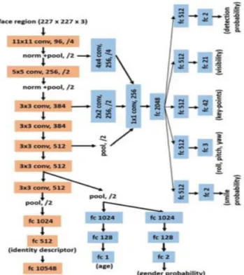
The All-in-one CNN model developed by Ranjan et al. (2017) is an example of a deeply supervised multi-task learning model implemented with remarkable success. The authors developed a multi-purpose algorithm, where face detection, face alignment, pose estimation, gender recognition, smile detection, age estimation and face recognition are performed simultaneously in a single deep CNN – the first of its kind - using a multi-task learning framework (MTL) which regularizes the parameters of the network. They achieve state-of-art results, using unconstrained datasets, in most of the proposed tasks (Ranjan, Sankaranarayanan, et al., 2017).

The method implemented in this paper has its basis on the MTL framework proposed by Caruana (Caruana, 1997). The lower layers parameters of the CNN are shared between all the tasks, as in this way, the lower layer learn a general and common representation to all the tasks performed, and the upper layers learn more abstract representations for the specific tasks. This approach has the potential to reduce over-fitting in the shared layers, and the process of learning robust features for different tasks makes it possible for the network to learn the correlations between data from different distributions in an effective way. The network has seven convolutional layers, followed by three fully connected ones. The first six convolution layers are used for the other face analysis tasks, sharing the parameters. The different specific tasks of the model are sub-models derived from different layers of the network. These sub-models are divided based on two definitions: whether the specific tasks rely on local – subject-independent - or global – subject-dependent - information of the face. The subject-independent tasks are face detection, key-points localization and visibility, pose estimation and smile prediction, and the subject-dependent tasks are age estimation, gender prediction and face recognition. The sub-model for subject-independent tasks fuse the first, third and fifth convolutional layers, as they rely more on local information, which can be seen as a more fundamental representation, available from the lower layers of the network. After the fused layers, two convolution, a pooling, and a fully-connected layer is added

(34)

22

specifically to these branched-out sub-model. After all these shared layers, a specific fully-connected layer is added to each different task, followed by the output layer. The sub-model for subject-dependent tasks are derived from the sixth convolutional layer, and three fully-connected layers are added to each specific task (Fig. 6) (Ranjan, Sankaranarayanan, et al., 2017).

The training of the All-in-one CNN contains five sub-networks with parameters shared among some of the tasks. Face detection, key-points localization and visibility, and pose estimation are trained as a single sub-model, as the same dataset is used for training them. The MTL approach used in the training of this sub-model is Task-based Regularization, where the optimal parameters for each task is obtained by minimizing the weighted sum of loss functions for each different task in the sub-model – where the weights are empirically assigned by the authors. The remaining tasks, smile detection, gender recognition, age estimation and face recognition are trained as separate sub-networks, as there is not a single large dataset with information regarding each task. The MTL approach in this case is Domain-based Regularization. With this method, the training is performed as if each model were a different CNN, but sharing the weights and updating them for each task. Doing so, the weights tend to adapt to the complete set of domains, instead of fitting to a task-specific domain, reducing over-fitting and making the model better at generalization (Ranjan, Sankaranarayanan, et al., 2017).

(35)

23

Figure 6 - Deeply supersized MTL architecture (Ranjan et al.,2017)

2.3.2. Parallel MTL architecture

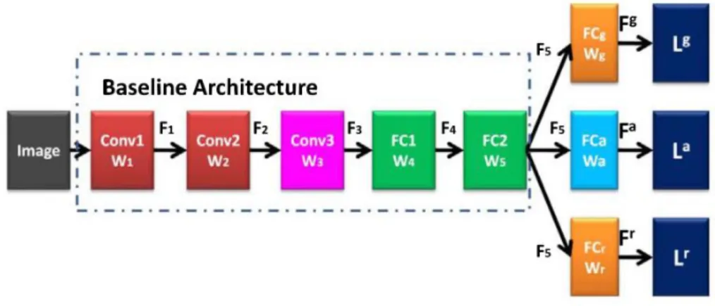
In the work of Xing et al. (2017), one of the proposed models has a parallel multi-task learning architecture. The proposed method sought to develop an age estimation model. During the development of the model, the authors proposed the incorporation of gender and race recognition in a multi-task learning framework as a means to further improve the age prediction task. By accumulating the insights of the proposed tasks, they obtained a very deep age estimation model that outperformed all the previous methods by a large margin (Xing et al., 2017).

They started with a baseline architecture based on AlexNet (Krizhevsky et al., 2012), which uses large convolution kernel and stride in the first layers, obtaining large feature maps, and gradually reducing its size as the layer goes deeper. The architecture has three convolutional layers, all of them consecutive with a max pooling layer, followed by two fully-connected layers (Fig. 7). The activation used is ReLu – Rectified Linear Units.

Having described the two most commonly used MTL approaches and outlined the main concepts and methods considered in the development of this study’s model with this literature review, a final section briefly presents a commercially available model.

(36)

24

Figure 7 - Parallel MTL architecture (Xing et al., 2017)

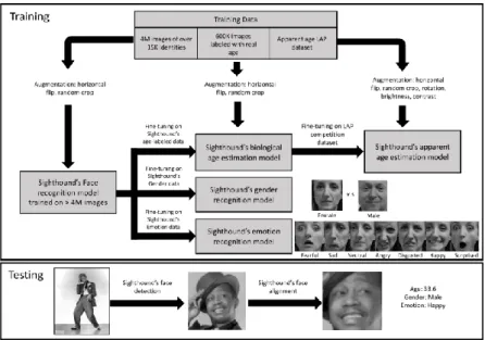
2.4. DAGER – a commercial approach

DAGER - Deep Age, Gender and Emotion Recognition, is a model developed by Dehghan et al. (2017). This is the only developed model with a somewhat similar output to the present dissertation. The model’s research paper describes the results of an end-to-end system developed for commercial use. Their system consists of several deep CNNs with the output tasks of Age, Gender and Emotion recognition on unconstrained real-world images (Fig. 8), without the use of any MTL approach. The CNNs internal mechanics, design, concepts and functions of choice are not shared, as this is a commercial software available through API calls to Sighthound’s server, with a cost up to 5000$ a month. They obtain state-of-the-art results on every task compared to other commercially available models, but the comparison is mostly done on their one proprietary dataset. The training data is proprietary and not available.

(37)

25

(38)

26

Chapter 3 – Methodology

After a complete review of the main concepts and techniques which were considered in the course of this study, the model proposition is outlined in this chapter. First, the model framework is described in respect to the conception of all the tasks, followed by the design of the network. Furthermore, the datasets used are outlined, with a description of the chosen split scheme and image processing. Lastly, the software for the implementation of this dissertation is discussed.

3.1. Task Formulation

During the next chapters, the methodology proposition for each task is outlined and explained. There are several ways to formulate each task, and several ways to design the model architecture. The final choice of model formulation for each task has a direct implication on the output of the network and can too have a direct implication on the model performance as some activation and loss functions are optimized for such tasks. First, a problem formulation for each task is given, explaining each choice, and then the score and loss functions are proposed. The choice of the baseline model architecture is, then, presented and described, as well as each single-task learning and multi-task learning frameworks.

3.1.1. Emotion recognition

The emotion recognition task is performed as a multi-class classification problem. As reviewed in the literature section, most databases incorporate seven distinct emotion classes: fear, anger, surprise, happiness, sadness, disgust and neutrality.

In the output layer, a loss function is needed as the training objective, to update the weights during the backpropagation stage. The most commonly used loss function deployed to train a multi-class mutually-exclusive problem is the multi-class cross-entropy loss. It indicates the distance between the output distribution. According to (Ranjan, Sankaranarayanan, et al., 2017), the cross-entropy loss is defined by equation 1:

ℒ

_{𝐸𝑚𝑜𝑡𝑖𝑜𝑛}

= ∑ −𝑦

_𝑐

𝑁−1

𝑐=0

(39)

27

Where 𝑁 is the number of classes, 𝑦𝑐 is the ground label of the sample, where 𝑦𝑐 = 1 if

the sample belongs to emotion 𝑐, otherwise 0, and at last 𝑝𝑐 is the predicted probability that

the sample belongs to emotion 𝑐. In this particular case, the equation (2) is modified.

ℒ

= ∑ −𝑦

_𝑐

6

𝑐=0

. log(𝑝

_𝑐

) (2)

Knowing that the ground truth label of the sample 𝑦 can only be one of the seven emotions (it is not a probability distribution), the other classes can be ignored and one can just use the matching term from the estimates 𝑦̂ (equation 3):

ℒ

= −𝑦

_{𝑒𝑚𝑜𝑡𝑖𝑜𝑛}

. log(𝑦

_{𝑒𝑚𝑜𝑡𝑖𝑜𝑛}

̂ ) (3)

Applying this to a determined number of samples 𝑁, as the input is a mini-batch (discussed in the next chapter), the loss is the average of all the input samples (equation 4):

ℒ

= −

1 𝑁

∑ 𝑦

𝑒𝑚𝑜𝑡𝑖𝑜𝑛𝑖

. log(𝑦

̂)

𝑖 𝑁

𝑖=1

(4)

The evaluation metrics used in this problem are accuracy, precision, recall and F1 score. Accuracy is used as it is the most common used metric in the development of classification problem CNNs, usually being the only model comparison method (in classification competitions such as Kaggle’s Facial Expression Recognition Challenge). Precision and recall are used to better evaluate the models, searching for biased accuracy results, and the F1 score, a function of precision and recall, which balances both results and is used with uneven class distributions.

3.1.2. Age estimation

The age estimation task can be drawn in three different formulations: as a multi-class classification problem, as a regression problem and as an ordinal regression problem. In the work of Xing et al. (2017), a comparison between these formulations is performed on the Morph II dataset using the same baseline architecture, and the best results are obtained treating the task as a regression problem. Aside from these results, treating the task as a regression problem is somewhat more natural, as the age of a human is measured in time after birth, therefore it is a real valued variable. The output layer of the task is composed of

(40)

28

only one neuron, contrary to the set of neurons needed if the problem was treated differently. Thus, the task of age estimation is treated as a regression problem.

The most used loss function in age estimation regression problems is the Mean Squared Error (MSE) –loss which is defined by equation 5:

ℒ

_𝐴𝑔𝑒

= (𝑦

̂ − 𝑦

_𝑎𝑔𝑒 _𝑎𝑔𝑒

)

2

(5)

Where N is the number of samples, 𝑦̂ is the prediction and 𝑦𝑎𝑔𝑒 _𝑎𝑔𝑒 is the ground truth

label.

Applying this to 𝑁 number of samples, the equation is 6:

ℒ

_𝐴𝑔𝑒

=

1 𝑁

∑ (𝑦

𝑎𝑔𝑒𝑖

̂ − 𝑦

𝑎𝑔𝑒𝑖

)

2 𝑁 𝑖=1

(6)

Where 𝑦̂_{𝑎𝑔𝑒𝑖} is the prediction and 𝑦_{𝑎𝑔𝑒𝑖} is the ground truth for the 𝑖𝑡ℎ_sample.

The evaluation metric used for this task is the Mean Absolute Error (MAE) metric, the most commonly used for regression problems and this task in particular.

3.1.3. Gender recognition

The task of gender recognition, as the task of emotion recognition, is a multi-class problem. There are two mutually exclusive classes – male or female. The loss function considered in this task is the same as in the emotion recognition task, the cross-entropy loss. Following the same basis described in the emotion recognition task, the loss is defined by the following equation:

ℒ

_{𝐺𝑒𝑛𝑑𝑒𝑟}

= −

1 𝑁

∑ 𝑦

𝑔𝑒𝑛𝑑𝑒𝑟 𝑖

. log (𝑦

𝑔𝑒𝑛𝑑𝑒𝑟𝑖

̂ )

𝑁

𝑖=1

(7)

Where 𝑁 is the number of samples, 𝑦̂𝑖 is the prediction and 𝑦𝑖 is the ground truth for the

𝑖𝑡ℎ_sample.

The evaluation metrics used in this problem are accuracy, precision, recall and F1 score, with the same motivation as explained in the emotion recognition task.

EAGLeNet - A Deep Multi-Task Learning CNN for Emotion, Age and Gender Recognition