Earthq Eng & Eng Vib (2012) 11: 553-566 DOI: 10.1007/s11803-012-0141-1
Comparative effi ciency analysis of different nonlinear modelling
strategies to simulate the biaxial response of RC columns
Hugo Rodrigues1,2†, Humberto Varum1‡, António Arêde3‡ and Aníbal Costa1§
1. University of Aveiro, Civil Engineering Department, Aveiro, Portugal
2. Faculty of Natural Sciences, Engineering and Technology - Oporto Lusophone University, Portugal 3.Civil Engineering Department, Faculty of Engineering, University of Porto, Portugal
Abstract:
The performance of different nonlinear modelling strategies to simulate the response of RC columns subjected to axial load combined with cyclic biaxial horizontal loading is compared. The models studied are classifi ed into two categories according to the nonlinearity distribution assumed in the elements: lumped-plasticity and distributed inelasticity. For this study, results of tests on 24 columns subjected to cyclic uniaxial and biaxial lateral displacements were numerically reproduced. The analyses show that the global envelope response is satisfactorily represented with the three modelling strategies, but signifi cant differences were found in the strength degradation for higher drift demands and energy dissipation.Keywords: RC columns; non-linear behaviour; biaxial bending; fi bre modelling
Correspondence to: Hugo Rodrigues, Civil Engineering
Department, University of Aveiro, Campus Universitário de Santiago, 3810-193 Aveiro, Portugal
Tel: +351 234 370049; Fax: +351 234 370094 E-mail: [email protected]
†Researcher; ‡Associate Professor; §FullProfessor
Supported by: Financial support provided by “FCT - Fundação
para a Ciência e Tecnologia,” Portugal, through the research project PTDC/ECM/102221/2008
Received March 29, 2012; Accepted October 15, 2012
1 Introduction
The philosophy applied in current seismic design codes and recommendations considers that buildings should respond elastically to small magnitude earthquakes, but for larger magnitudes a nonlinear structural response is explored. Thus, there is a current need for accurate nonlinear models to account for the hysteretic behavior of reinforced concrete (RC) structures (Duarte, 1991). The determination of the effects of earthquakes on buildings generally requires the consideration of two horizontal component loads in columns, which tend to induce larger demands than one-directional actions. In many situations, biaxial demands on columns also result in the torsional response of buildings, namely as a result of in-plane structural irregularities (Romão et al., 2004).
With regard to the modeling of RC members under cyclic 2D bending combined with axial load, current knowledge is still far behind that for uniaxial bending, and many questions need to be verifi ed in the modelling of the biaxial response of RC elements. Different modelling strategies have been proposed for the
simulation of the biaxial cyclic behavior of RC elements with axial force. A detailed review of the available models is presented in CEB (1996) and Fardis (1991). In addition to the fi ber models (Petrangeli et al., 1999; Taucer et al., 1991; Spacone et al., 1992), other analytical models are available, following the concepts of classical plasticity (Pecknold, 1974), Mroz multisurface plasticity (Takizawa and Aoyama, 1976; Powell and Chen, 1986; Galal and Ghobarah, 2003), Bouc-Wen (Wen, 1976), hysteresis modelling (Romão et al., 2004; Kunnath and Reinhorn, 1990; Casciati, 1989; Wang and Wen, 2000), bounding surface plasticity (Sfakianakis and Fardis, 1991a, 1991b; Bousias et al., 2002), or lumped damage models (Marante and Florez-Lopez, 2002, 2003; Mazza and Mazza, 2008), among others. The available test results for biaxial bending are not as extensive and the development and calibration is not exhaustive.
This study intends to evaluate and compare the adequacy of different nonlinear modelling strategies in the representation of RC columns’ response when subjected to axial force combined with cyclic biaxial horizontal loading.
2 Specimen description and testing conditions
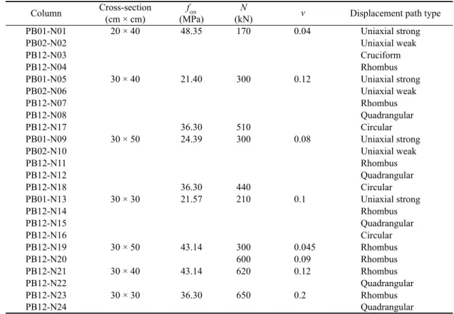
Rodrigues et al. (2010) carried out an experimental campaign on 24 full-scale RC columns, tested under uniaxial and biaxial cyclic loading. The specimens consisted of RC columns built as a cantilever cast in a heavily reinforced foundation. The columns were subjected to constant axial load and cyclic lateral loading imposed under displacement controlled conditions. The general characteristics of the specimensand testing conditions are summarized in Table 1. A more detailed description of the columns’ geometry, material properties, reinforcement details and test results is reported in (Rodrigues et al., 2012). The general characteristics of the specimens and testing conditions are summarized in Fig. 1.
In order to characterize the response of the column specimens, cyclic lateral displacements were imposed at the top of the column with steadily increasing demand levels. In the biaxial tests, four different patterns for the demands history were considered, namely one in which the displacement cycles are applied alternately in the two horizontal directions (cruciform path), one with an expanding rhombus shape, one expanding square centered in the origin and fi nally a circular load path. Three cycles were repeated for each lateral deformation demand level. This procedure allows for an understanding of the column’s behavior and a comparison between different tests. It provides information for the development and calibration of numerical models; in this case, the following nominal peak displacement levels were considered in the directions of loading (x and y): 3, 5, 10, 4, 12, 15, 7, 20, 25, 30, 35, 40, 45, 50, 55, 60, 65, 70, 75, 80 (Rodrigues et al., 2010, 2012c). For all the tests, the fi rst branch of the load path is imposed in the direction (X) of the column.
For each test on the column specimens, the following general designation “PB$$-N##” was adopted, where:
• $$ takes the value “01” for the test in the
column’s strong direction (X), the value “02” for the
weak direction test (Y), and the value “12” for the biaxial test;
• ## represents the reference number of the
column specimen.
3 Numerical tool and modelling strategies
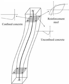
The numerical analyses developed and described in this paper with different nonlinear modelling strategies were performed using the computer program SeismoStruct (SeismoSoft, 2004). The program includes models for the representation of the behavior of spatial frames under static and/or dynamic loading, considering both material and geometric nonlinearities. With the software, seven types of analyses can be performed, namely: dynamic and static time-history analysis, conventional and adaptive pushover, incremental dynamic analysis, modal analysis, and static analysis (possibly nonlinear) under quasi-permanent loading. The software allows for the use of elements with distributed inelasticity (force or displacement-based formulations) and elements with lumped-plasticity (with fi xed length, so-called plastic-hinge). Fiber discretization is adopted to represent the behavior at the section level (see Fig. 2), where each fi ber is associated with a uniaxial stress-strain law. The sectional moment-curvature state of the beam and column elements is then obtained through the integration of the nonlinear uniaxial stress-strain response of the individual fi bers into which the section has been subdivided.Table 1 Specimen description and testing conditions
Column Cross-section(cm × cm) fcm (MPa)
N
(kN) ν Displacement path type
PB01-N01 20 × 40 48.35 170 0.04 Uniaxial strong PB02-N02 Uniaxial weak PB12-N03 Cruciform PB12-N04 Rhombus PB01-N05 30 × 40 21.40 300 0.12 Uniaxial strong PB02-N06 Uniaxial weak PB12-N07 Rhombus PB12-N08 Quadrangular PB12-N17 36.30 510 Circular PB01-N09 30 × 50 24.39 300 0.08 Uniaxial strong PB02-N10 Uniaxial weak PB12-N11 Rhombus PB12-N12 Quadrangular PB12-N18 36.30 440 Circular PB01-N13 30 × 30 21.57 210 0.1 Uniaxial strong PB12-N14 Rhombus PB12-N15 Quadrangular PB12-N16 Circular PB12-N19 30 × 50 43.14 300 0.045 Rhombus PB12-N20 600 0.09 Rhombus PB12-N21 30 × 40 43.14 620 0.12 Rhombus PB12-N22 Quadrangular PB12-N23 PB12-N24 30 × 30 36.30 650 0.2 Rhombus Quadrangular
3.1 Numerical modelling strategies
In this work, three nonlinear modelling strategies are compared, based on: elements with lumped-plasticity (Fig. 3a); elements with distributed inelasticity and force-based formulation (Fig. 3(b)); and elements with distributed inelasticity and displacement-based formulation (Fig. 3(c)). The three modelling strategies were applied to each column specimen and the obtained results were compared.
Decisions for each modelling strategy were taken based on the results of parametric studies performed by other authors (Taucer et al., 1991; Calabrese, 2008; Calabrese et al., 2010), as described next.
Different studies have proposed expressions to
estimate the plastic hinge length (Lp) of RC elements to be adopted in lumped plasticity models (Bae and Bayrak, 2008). Priestley and Park (1987) proposed a formulation that estimates the plastic hinge length based on the distance of the critical section from the point of contrafl exure and on the diameter of the longitudinal reinforcement bars. Based on this formulation, Paulay and Priestley (1992) reported that for typical RC columns, the plastic hinge length is approximately equal to half of the cross-section depth. Thus, in the simulations performed for the uniaxial tests, the plastic hinge length was considered equal to half of the cross-section depth. For the biaxial tests, based on experimental evidence, other authors have concluded that the plastic hinge length is not strongly affected by 2D loading (Tsuno and Park, 2004). The plastic hinge length in rectangular columns under biaxial loading approximately assumes the length observed in the column tested uniaxially in its strong direction as observed by (Rodrigues et al., 2012a). In the analyses performed in this study, half of the larger dimension of the cross-section was considered as the plastic hinge length.
For the force based formulation, seven integration points were considered, based on the results of Calabrese
et al. (2010). These authors point out that at least six
integration sections are needed in order to obtain a completely stabilized prediction of the local response.
According to the results of Calabrese et al. (2010), for displacement based formulations, a good approximation to a cantilever column response can be obtained with a mesh discretization of at least four elements, with two Gauss-Legendre points per element, if all elements have the same length. Considering this and taking into account the concentration of the nonlinear response close to the fi xed end of the column (plastic hinge length), a discretization of the column in six elements with the length presented in Fig. 3 was adopted.
Fig. 1 RC column specimen dimensions and reinforcement detailing 2Ø10 9Ø16 9Ø16 0.11 0.15 9Ø16 2Ø10 0.08 9Ø16 Ø12 0.15 0.1 1.2 0.5 0.2 0.3 0.3 0.3 0.4 0.4 0.5 0.3 10Ø12 14Ø12 8Ø12 Ø6/0.15 Ø6/0.15 Ø6/0.15 Ø6/0.075
Fig. 2 Fiber based modelling
Reinforcement steel
Unconfi ned concrete Confi ned concrete
3.2 Material properties and section models
The consideration of nonlinear material behavior in the prediction of the RC columns’ response requires accurate modelling of the uniaxial material stress-strain cyclic response. In the present section, the concrete and reinforcing steel constitutive models used and the value considered for each parameter are presented.
3.2.1 Concrete
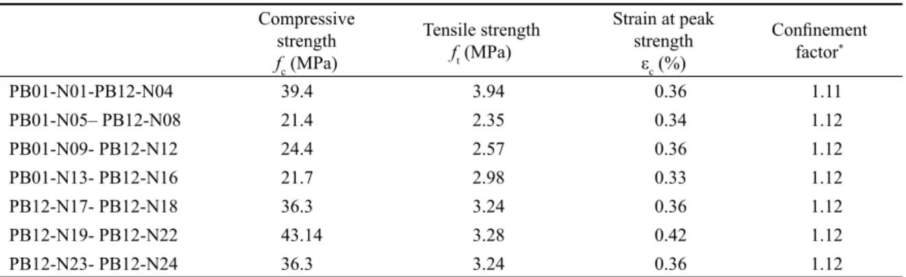
For the concrete, a model based on the Madas and Elnashai (1992) uniaxial model, which follows the constitutive law proposed by Mander et al. (1988), is used. The cyclic rules included in the model for the confi ned and unconfi ned concrete were proposed by Martinez-Rueda and Elnashai (1997). The confi nement effects provided by the transverse reinforcement were considered through the rules proposed by Mander et al. (1988), whereby constant confi ning pressure is assumed throughout the entire stress-strain range, indicated by the increase in the peak value of the compression strength and the stiffness of the unloading branch (SeismoSoft, 2004). The input parameters of the model for the concrete are:
compressive strength (fc), tensile strength (ft), the strain at peak strength (εc) and the confi nement factor. All the adopted values are in accordance with the properties obtained in the material tests (Rodrigues et al., 2010). Table 2 presents the properties considered in the numerical models. Material mechanical parameters were defi ned based on test results on samples (Rodrigues
et al., 2010).
3.2.2 Reinforcement steel
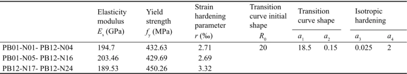
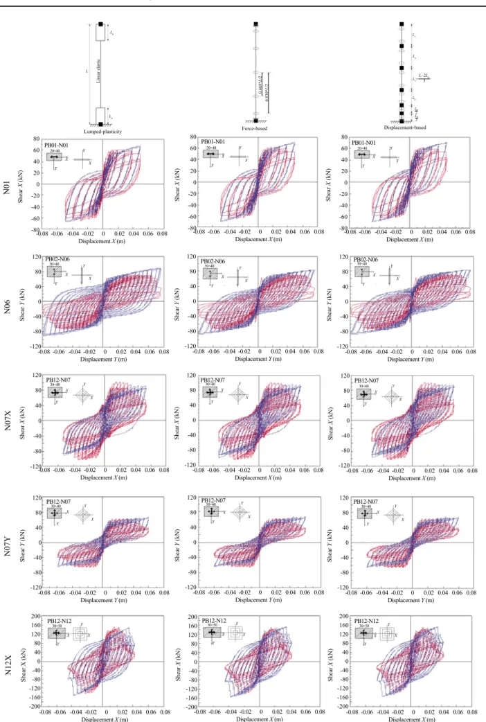
The uniaxial model proposed by Menegotto and Pinto (1973), coupled with the isotropic hardening rules proposed by Filippou et al. (1983), was adopted for the steel reinforcement. This steel model does not represent the yielding plateau characteristic of the mild steel virgin curve. The model takes into account the Bauschinger effect, which is relevant for the representation of the columns’ stiffness degradation under cyclic loading. The input parameters of the model are: the yield strength (fy); the elastic Young modulus (Es); the strain-hardening ratio (r) and fi ve parameters to describe the transition from elastic to plastic Fig. 3 Modelling strategies with indication of the control section points: (a) lumped-plasticity element; (b) distributed inelasticity element with force-based formulation; (c) distributed inelasticity element with displacement-based formulation
Node Integration point Lp Lp La La La= Lp Lp 2 Lp 2 L–2Lp 3 0.469* L /2 0.830* L /2 Linear elastic L (a) (b) (c)
Table 2 Concrete mechanical parameters for the numerical models
Compressive strength fc (MPa) Tensile strength ft (MPa) Strain at peak strength εc (%) Confi nement factor* PB01-N01-PB12-N04 39.4 3.94 0.36 1.11 PB01-N05– PB12-N08 21.4 2.35 0.34 1.12 PB01-N09- PB12-N12 24.4 2.57 0.36 1.12 PB01-N13- PB12-N16 21.7 2.98 0.33 1.12 PB12-N17- PB12-N18 36.3 3.24 0.36 1.12 PB12-N19- PB12-N22 43.14 3.28 0.42 1.12 PB12-N23- PB12-N24 36.3 3.24 0.36 1.12
branches (R0, a1, a2, a3, and a4). The model parameters considered are summarized in Table 3. All the adopted values are in accordance with the properties obtained in the material tests (Rodrigues et al., 2010). Table 2 presents the properties considered in the numerical models.Material mechanical parameters were defi ned based on test results on samples (Rodrigues et al., 2010).
4 Comparison between modelling strategies
The three modelling strategies were used to reproduce the response of the specimens tested. For the parameters controlling the cyclic response of the reinforcement steel, the default values were adopted as indicated in the software manual (SeismoSoft, 2004) and specifi ed in Table 3. For each column analyzed, the axial load and the corresponding horizontal displacement law were imposed in accordance with the experimental results. The numerical results for each modelling strategy were compared with the experimental results and are discussed in the next sections.
4.1 Shear-drift envelopes
The experimental shear-drift envelope curve obtained for each column is compared with the results of the nonlinear models in terms of initial stiffness, and evolutions of tangent and secant stiffness.
Figure 4 presents, as an example, the shear-drift envelopes in one direction for the columns with cross-sectional dimensions of 30cm×50cm for uniaxial and biaxial tests (columns N09 to N12 and N18). From the analysis of the shear-drift envelopes, a good agreement was found in the numerical representation of the experimentally measured response. The differences found between the different modelling strategies are discussed next.
4.1.1 Global comparison
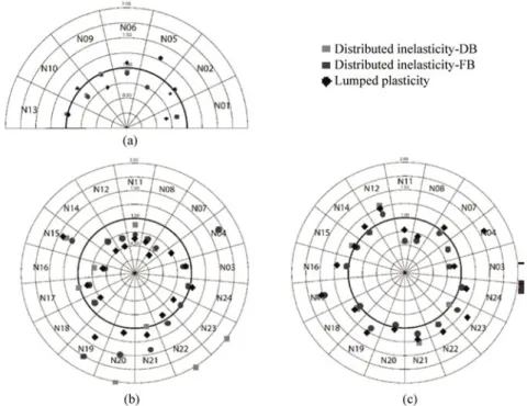
In order to compare the envelopes obtained with the experimental results and with the numerical models, the correlation coeffi cient (R2) was calculated. As usual, the statistical measure R2 assumes the value of 1.0 when a perfect correlation between the numerical and experimental data is found. In these comparisons, by convention, 0.75 is established as the minimum R2 value for a good fi t. Based on the obtained R2 results for all analyses, presented in Fig. 5, the following can be concluded:
• For the majority of numerical analyses performed, correlation coeffi cients higher than 0.75 were obtained, indicating a good representation of the experimental envelopes.
• For each studied column, similar correlation coeffi cients were found with the three modelling strategies. However, the modelling strategy with the lumped plasticity element presents the lowest correlation coeffi cients.
• For all columns analyzed under biaxial demands, the correlation coeffi cient for the strong (X) and weak (Y) directions is similar.
4.1.2 Initial stiffness comparison
The initial stiffness of the column evaluated from the shear drift envelope curves obtained with the different numerical models was compared with the corresponding initial stiffness derived from the experimental tests. Figure 6 shows the ratio between the experimental and numerical initial stiffness obtained for all columns, from which the following can be concluded:
• For the uniaxial tests, the ratio assumes values close to 1, indicating that all models represent the columns’ initial stiffness well, with a maximum sub-evaluation of about 25%.
• For the biaxial results, a higher dispersion was found in the calculated initial stiffness, with a sub-evaluation in the column strong direction (around 25%–50%) and an over-evaluation in the weak direction (around 25%).
• For the biaxial tests, the distributed plasticity model with the force based formulation gave the worst estimate of the initial stiffness.
4.1.3 Secant stiffness comparison
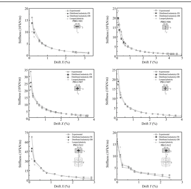
The evolution of the columns’ secant stiffness with the drift demand was evaluated by comparing the peak-to-peak secant stiffness of the fi rst cycle of each drift demand level. Figure 7 shows examples of the reduction in secant stiffness with drift demand for the columns PB01-N1, PB02-N6, PB12-N7, and PB12-N12. The secant stiffness evolution for all the tested columns was compared with the corresponding values obtained with the numerical models developed. Regardless of the displacement history (uniaxial or any path for biaxial loading), the secant stiffness evolution obtained from the tests is captured very well by all the modelling strategies.
4.1.4 Tangent stiffness comparison
The evolution of the tangent stiffness determined Table 3 Steel mechanical parameters for the numerical models
Elasticity modulus Es (GPa) Yield strength Strain hardening parameter Transition curve initial shape Transition curve shape Isotropic hardening fy (MPa) r (‰) R 0 a1 a2 a3 a4 PB01-N01- PB12-N04 194.7 432.63 2.71 20 18.5 0.15 0.025 2 PB01-N05- PB12-N16 203.46 429.69 2.69 PB12-N17- PB12-N24 189.53 450.26 3.32
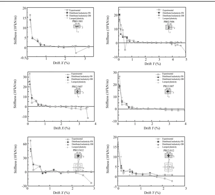
from the shear-drift envelope curves was analyzed for all the studied columns of the fi rst cycle of each drift demand level. Figure 8 shows examples of the tangent stiffness evolutions (experimental and numerical) with the drift demands, namely for columns PB01-N1, PB02-N6, PB12-N7, and PB12-N12. From the results obtained
for all columns, the following was observed:
• The tangent stiffness presents similar evolutions for the three modelling strategies.
• Compared with the experimental results, numerical models show diffi culties in representing the tangent stiffness for lower drift demands (less than
Fig. 4 Shear-drift envelopes for 30cm×50cm columns (measured and calculated). FB - distributed inelasticity-displacement-base
formulation, DB - distributed inelasticity-force-base formulation, LP – lumped plasticity
200 175 150 125 100 75 50 25 0 Shear X (kN) 0 1 2 3 4 Drift X (%) PB01-N09 Experimental Numerical-FB Numerical-DB Numerical-LP 200 175 150 125 100 75 50 25 0 Shear Y (kN) 0 1 2 3 4 5 6 Drift Y (%) PB02-N10 Experimental Numerical-FB Numerical-DB Numerical-LP 200 175 150 125 100 75 50 25 0 Shear X (kN) 0 1 2 3 4 Drift X (%) PB12-N11 Experimental Numerical-FB Numerical-DB Numerical-LP 200 175 150 125 100 75 50 25 0 Shear Y (kN) 0 1 2 3 4 Drift Y (%) PB12-N11 Experimental Numerical-FB Numerical-DB Numerical-LP 200 175 150 125 100 75 50 25 0 Shear X (kN) 0 1 2 3 4 Drift X (%) PB12-N12 Experimental Numerical-FB Numerical-DB Numerical-LP 200 175 150 125 100 75 50 25 0 Shear Y (kN) 0 1 2 3 4 Drift Y (%) PB12-N12 Experimental Numerical-FB Numerical-DB Numerical-LP 200 175 150 125 100 75 50 25 0 Shear X (kN) 0 1 2 3 4 Drift X (%) PB12-N18 Experimental Numerical-FB Numerical-DB Numerical-LP 200 175 150 125 100 75 50 25 0 Shear Y (kN) 0 1 2 3 4 Drift Y (%) PB12-N18 Experimental Numerical-FB Numerical-DB Numerical-LP Y X X Y Y X X Y 30×50 Y X X Y 30×50 30×50 30×50 30×50 30×50 30×50 30×50 Y X X Y Y X X Y Y X X Y Y X X Y Y X X Y
Fig. 6 Initial stiffness ratio between experimental and numerical results: (a) uniaxial texts; (b) biaxial tests – strong direction (X); (c) biaxial tests – weak direction (Y)
Fig. 5 Correlation coeffi cients of shear-drift envelopes between experimental and numerical results (R2): (a) uniaxial texts; (b)
biaxial tests – strong direction (X); (c) biaxial tests – weak direction (Y)
1%). The diffi culties in representing the initial behavior were already reported in the analysis of the differences obtained for the initial stiffness.
• For drift demands larger than 1%, a good representation of the tangent stiffness evolution is reached with the numerical models, corresponding to a plateau in the post-yielding zone (approximately zero stiffness). However, for drift demands larger than those corresponding to the beginning of the column strength
degradation, the numerical models do not accurately represent the tangent stiffness evolution. This aspect is more evident for the columns under biaxial loading conditions, since the strength degradation starts for lower drift demands, as seen in the examples presented in Fig. 8, where the post-yielding plateau is shorter.
4.2 Cyclic response
Fig. 7 Secant stiffness evolution for columns PB01-N1, PB02-N6, PB12-N7, and PB12-N12: Experimental and numerical results. 20 15 10 5 0 Stif fness (10 3kN/m) Experimental Distributed inelasticity-FB Distributed inelasticity-DB Lumped plasticity 0 1 2 3 Drift X (%) PB01-N01 25 20 15 10 5 0 Stif fness (10 3kN/m) Experimental Distributed inelasticity-FB Distributed inelasticity-DB Lumped plasticity 0 1 2 3 4 5 Drift Y (%) PB02-N06 35 30 25 20 15 10 5 0 Stif fness (10 3kN/m) Experimental Distributed inelasticity-FB Distributed inelasticity-DB Lumped plasticity 0 1 2 3 4 Drift X (%) PB12-N07 25 20 15 10 5 0 Stif fness (10 3kN/m) Experimental Distributed inelasticity-FB Distributed inelasticity-DB Lumped plasticity 0 1 2 3 4 Drift Y (%) PB12-N07 75 60 45 30 15 0 Stif fness (10 3kN/m) Experimental Distributed inelasticity-FB Distributed inelasticity-DB Lumped plasticity 0 1 2 3 Drift X (%) PB12-N12 20 15 10 5 0 Stif fness (10 3kN/m) Experimental Distributed inelasticity-FB Distributed inelasticity-DB Lumped plasticity 0 1 2 3 Drift Y (%) PB12-N12
representation of the cyclic response of the RC columns under study is evaluated. Examples of shear-drift responses comparing experimental and numerical results are presented in Fig. 9, namely for columns PB01-N1, PB02-N6, PB12-N7, and PB12-N12.
4.2.1 Overall analysis
The general analysis of the cyclic response of the columns obtained with the three modelling strategies and the comparison with the corresponding experimental results show that:
• Even when a good representation of the global columns’ response is achieved, the numerical response may not adequately capture the strength degradation for the largest deformation demands, which is associated with the buckling of the reinforcing steel bars.
• In many cases, the unloading-reloading phase of the columns’ cyclic response obtained with the numerical models does not accurately capture the pinching effect observed experimentally. This can be justifi ed by the limitations of the models in the representation of the longitudinal reinforcing steel slippage.
4.2.2 Shear force evolution
In order to evaluate the accuracy of the numerical models studied in the representation of the shear force evolution obtained experimentally, the frequency domain error (FDE) index (Lepage et al., 2010; Dragovich and Lepage, 2009) was calculated. The FDE index (Dragovich and Lepage, 2009) measures the deviation between two waveforms, in this case the shear force measured in the test and the corresponding calculated shear force for each modelling strategy. The FDE index quantifi es amplitude and phase deviations between two signals, giving an error factor with a value between 0 and 1. In this analysis, it is considered that a FDE index larger than 0.75 represents a poor correlation and a value below 0.25 represents a very good correlation. These limits were proposed in (Lepage et al., 2010).
The FDE indices obtained for all analyses are represented in Fig. 10. From the analysis of the results, the following conclusions can be drawn:
• For all columns studied, with uniaxial and biaxial loading, the three developed numerical models
X Y 20×40 X Y 30×40 X Y 30×40 X Y 30×40 X Y 30×50 Y X X X Y Y 30×50
Fig. 8 Tangent stiffness evolution for columns PB01-N1, PB02-N6, PB12-N7, and PB12-N12: Experimental and numerical results 20 15 10 5 0 -0.5 Stif fness (10 3kN/m) Experimental Distributed inelasticity-FB Distributed inelasticity-DB Lumped plasticity 0 1 2 3 Drift X (%) PB01-N01 20 10 0 -10 Stif fness (10 3kN/m) Experimental Distributed inelasticity-FB Distributed inelasticity-DB Lumped plasticity 0 1 2 3 4 5 Drift Y (%) PB02-N06 30 20 10 0 -10 Stif fness (10 3kN/m) Experimental Distributed inelasticity-FB Distributed inelasticity-DB Lumped plasticity 0 1 2 3 4 Drift X (%) PB12-N07 30 20 10 0 -10 Stif fness (10 3kN/m) Experimental Distributed inelasticity-FB Distributed inelasticity-DB Lumped plasticity 0 1 2 3 4 Drift Y (%) PB12-N07 60 30 0 -30 Stif fness (10 3kN/m) Experimental Distributed inelasticity-FB Distributed inelasticity-DB Lumped plasticity 0 1 2 3 Drift X (%) PB12-N12 20 15 10 5 0 -5 Stif fness (10 3kN/m) Experimental Distributed inelasticity-FB Distributed inelasticity-DB Lumped plasticity 0 1 2 3 Drift Y (%) PB12-N12
adequately represent the shear force evolutions recorded in the experimental tests. The calculated FDE index was slightly larger than 0.25. Moreover, no signifi cant differences were found in the FDE index for the three modelling strategies applied to each column tested.
• For all columns analyzed under biaxial demands, the FDE index is lower in the weak direction (Y) than in the strong direction (X), which is in accordance with the larger differences identifi ed in this direction in terms of stiffness evolution and strength degradation.
4.2.3 Cumulative energy dissipation
The accuracy of the nonlinear models is characterized here in terms of the total energy dissipated, comparing the values calculated with the numerical models with the values obtained from the tests on columns. Figure 11 shows examples of the evolution of the cumulative dissipated energy and Fig. 12 shows the ratio between the numerical and experimental values of the total energy dissipated. Based on the obtained results, the following can be concluded:
• Generally, for the columns analyzed
under uniaxial loading conditions, a considerable overestimation of the total energy dissipated was obtained with the numerical models (Fig. 12(a)). This effect was not observed in any column under biaxial loading. The overestimation of the energy dissipated is justifi ed by the inadequacy of the numerical models in the strength degradation representation.
• Results for the columns with biaxial loading, analyzed for each direction independently, show a variation in the total energy dissipated between 25% and 50% (Figs. 12(c) and 11(d)), being larger for the weak direction (Y).
• The sum of the total energy dissipated in each direction (Fig. 12(b)) demonstrates, generally, an overestimation with the adopted numerical strategies studied. For columns N22, N23, and N24, the higher axial load level anticipates the collapse for lower drift demands, and therefore, the total energy dissipated calculated from the numerical response underestimates the experimental value. This is justifi ed by the decreased adequacy of the models in accurately representing the
X Y 30×50 X Y 30×50 X Y X Y 30×40 X Y 30×40 X Y 20×40 X Y 30×40 X Y
80 60 40 20 0 -20 -40 -60 -80 Shear X (kN) -0.08 -0.06 -0.04 -0.02 0 0.02 0.04 0.06 0.08 Displacement X (m) PB01-N01 80 60 40 20 0 -20 -40 -60 -80 Shear X (kN) -0.08 -0.06 -0.04 -0.02 0 0.02 0.04 0.06 0.08 Displacement X (m) PB01-N01 80 60 40 20 0 -20 -40 -60 -80 Shear X (kN) -0.08 -0.06 -0.04 -0.02 0 0.02 0.04 0.06 0.08 Displacement X (m) 120 80 40 0 -40 -80 -120 Shear Y (kN) -0.08 -0.06 -0.04 -0.02 0 0.02 0.04 0.06 0.08 Displacement Y (m) PB02-N06 120 80 40 0 -40 -80 -120 Shear Y (kN) -0.08 -0.06 -0.04 -0.02 0 0.02 0.04 0.06 0.08 Displacement Y (m) PB02-N06 120 80 40 0 -40 -80 -120 Shear Y (kN) -0.08 -0.06 -0.04 -0.02 0 0.02 0.04 0.06 0.08 Displacement Y (m) PB02-N06 120 80 40 0 -40 -80 -120 Shear X (kN) -0.08 -0.06 -0.04 -0.02 0 0.02 0.04 0.06 0.08 Displacement X (m) PB12-N07 120 80 40 0 -40 -80 -120 Shear X (kN) -0.08 -0.06 -0.04 -0.02 0 0.02 0.04 0.06 0.08 Displacement X (m) PB12-N07 120 80 40 0 -40 -80 -120 Shear X (kN) -0.08 -0.06 -0.04 -0.02 0 0.02 0.04 0.06 0.08 Displacement X (m) PB12-N07 120 80 40 0 -40 -80 -120 Shear Y (kN) -0.08 -0.06 -0.04 -0.02 0 0.02 0.04 0.06 0.08 Displacement Y (m) PB12-N07 120 80 40 0 -40 -80 -120 Shear Y (kN) -0.08 -0.06 -0.04 -0.02 0 0.02 0.04 0.06 0.08 Displacement Y (m) PB12-N07 120 80 40 0 -40 -80 -120 Shear Y (kN) -0.08 -0.06 -0.04 -0.02 0 0.02 0.04 0.06 0.08 Displacement Y (m) PB12-N07 200 160 120 80 40 0 -40 -80 -120 -160 -200 Shear X (kN) -0.08 -0.06 -0.04 -0.02 0 0.02 0.04 0.06 0.08 Displacement X (m) PB12-N12 200 160 120 80 40 0 -40 -80 -120 -160 -200 Shear X (kN) -0.08 -0.06 -0.04 -0.02 0 0.02 0.04 0.06 0.08 Displacement X (m) PB12-N12 200 160 120 80 40 0 -40 -80 -120 -160 -200 Shear X (kN) -0.08 -0.06 -0.04 -0.02 0 0.02 0.04 0.06 0.08 Displacement X (m) PB12-N12 N01 N06 N07X N07Y N12X Lp Lp ??????????????? Force-based Displacement-based Lumped-plasticity
Fig. 9 Shear-drift response for columns PB01-N1, PB02-N6, PB12-N7, and PB12-N12: Experimental and numerical results
20×40 X Y Y X 20×40 X Y Y X PB01-N01 20×40 X Y Y X 20×40 X Y Y X X Y Y X 30×40 30×40 30×40 X Y Y X 30×40 X Y Y X 30×40 X Y Y X 30×40 X Y Y X 30×40 X Y Y X X Y Y X 30×40 X Y Y X 30×40 30×50 X Y Y X 30×50 X Y Y X 30×50 X Y Y X 0.469* L /2 0.830* L /2 Lp Lp Linear elastic L La La La= Lp Lp 2 Lp 2 L–2Lp 3
Fig. 9 Continued
Fig. 10 FDE index obtained from the comparison between numerical and experimental shear force evolutions: (a) uniaxial tests; (b) biaxial tests – strong direction (X); (c) biaxial tests – weak direction (Y)
energy dissipation for lower deformations associated with a quasi-linear numerical response in this stage.
• For each studied column under biaxial loading conditions, similar ratios were obtained with the three modelling strategies. However, for the weak direction, the model with distributed plasticity with a force-based formulation presents higher differences in the total energy dissipated. Comparing the sum of the total energy dissipated in both directions, the lumped plasticity modelling strategy presents larger deviations.
5 Conclusions
In this study, the adequacy of three modelling strategies in the representation of RC columns’ responses under uniaxial and biaxial loading conditions was analyzed.
From the analysis of the obtained results, similar levels of adequacy were verifi ed using the distributed inelasticity (force and displacement formulations) and the lumped plasticity modelling strategies. However,
based on the comparisons made, the following conclusions can be drawn:
• The initial stiffness obtained with all the modelling strategies for the simulation of the biaxial tests presents differences, when compared with the experimental values, in the range of 25% to 50%.
• The secant stiffness evolution of the columns was accurately represented with all modelling strategies. However, considerable differences were observed between the numerical and experimental tangent stiffness evolutions, mainly for the lower drift demands and in the last phase of the columns’ responses. This aspect confi rms the diffi culties normally found in numerically representing the response of columns with models based on incremental procedures, which depend on the tangent stiffness.
• The cyclic response obtained with the three modelling strategies for all columns was found to be satisfactory, but diffi culties were found in capturing the strength degradation for the higher drift demands. Also, the majority of the models show limitations in representing the pinching effect in the
unloading-reloading stage.
• All modelling strategies exhibit diffi culties in the representation of the energy dissipation evolution. The difference in the total dissipated energy was found to range between 25% and 50%. The main differences correspond to an underestimation of the dissipated energy for lower drift demands associated with a quasi-linear numerical response and to an overestimation for higher demands associated with the limitations of the numerical models in the representation of the strength degradation and pinching effect.
Finally, it is worth emphasizing that many questions are still open in the modelling of the biaxial response of RC columns. The modelling strategies analyzed in this paper can accurately predict the cyclic response of the columns until the strength degradation begins. This aspect is not so relevant for uniaxial loading, since strength degradation starts for larger drift demands in comparison with biaxial loadings.
RC structural models should be further developed for a more rigorous consideration of the steel reinforcing bars’ behavior for larger drift demands, in order to accurately represent the bar buckling, which will
improve the simulation of strength degradation. Some proposals are listed in the References, but these models depend on parameters for which a precise calibration should be developed.
All modelling strategies studied show similar deviations to the response of the columns obtained in the experimental tests. This points towards the use of a lumped plasticity modelling strategy for the representation of RC elements, since the strategy is simple and the element discretization is only dependent on the plastic hinge length, which has a direct physical interpretation. Furthermore, in applications for the analysis of complex RC building structures, the lumped plasticity modelling strategies lead to more reduced computational time and the analysis is concentrated on the critical sections in the element.
Acknowledgment
The authors acknowledge the LESE laboratory staff, particularly Valdemar Luís, André Martins and Engº Luís Noites, for their support in the preparation and Fig. 11 Evolution of the cumulative dissipated energy for columns PB01-N1, PB02-N6, PB12-N7, and PB12-N12: Experimental and numerical results
40 30 20 10 0 Experimental Distributed inelasticity-FB Distributed inelasticity-DB Lumped plasticity PB01-N01 250 200 150 100 50 0 Experimental Distributed inelasticity-FB Distributed inelasticity-DB Lumped plasticity PB02-N06 125 100 75 50 25 0 Experimental Distributed inelasticity-FB Distributed inelasticity-DB Lumped plasticity Step PB12-N07 125 100 75 850 25 0 Experimental Distributed inelasticity-FB Distributed inelasticity-DB Lumped plasticity PB12-N07 175 150 125 100 75 50 25 0 Dissipated ener gy X direction (kN . m) Experimental Distributed inelasticity-FB Distributed inelasticity-DB Lumped plasticity PB12-N12 175 150 125 100 75 50 25 0 Experimental Distributed inelasticity-FB Distributed inelasticity-DB Lumped plasticity PB12-N12 Step Step Dissipated ener gy Y direction (kN . m) Dissipated ener gy X direction (kN . m) Dissipated ener gy Y direction (kN . m) Dissipated ener gy (kN . m) Dissipated ener gy (kN . m) Experimental Distributed inelasticity-FB Distributed inelasticity-DB Lumped plasticity PB12-N12 20×40 X Y 30×40 X Y 30×40 X Y 30×50 X Y 30×50 X Y X Y Y X 30×40 X Y
Fig.12 Ratio between the total dissipated energy obtained with the numerical models and the experimental value: (a) uniaxial tests; (b) biaxial tests – total (X + Y); (c) biaxial tests – strong direction (X); (d) biaxial tests – weak direction (Y)
implementation of the testing set-up. This paper reports research developed under fi nancial support provided by “FCT - Fundação para a Ciência e Tecnologia,” Portugal, namely through the PhD grants of the fi rst author with reference SFRH/BD/63032/2009 and through the research project PTDC/ECM/102221/2008.
References
Bae S and Bayrak O (2008), “Plastic Hinge Length of Reinforced Concrete Columns,” ACI Structural Journal,
105: 290–300.
Bousias SN, Panagiotakos TB and Fardis MN (2002), “Modelling of RC Members under Cyclic Biaxial Flexure and Axial Force,” Journal of Earthquake
Engineering, 6(2): 213–238.
Calabrese A (2008), “Numerical Issues in Distributed Inelasticity Modelling of RC Frame Elements for Seismic Analysis,” MsC, Istituto Universitario di Studi Superiori di Pavia, Università degli Studi di Pavia, Pavia.
Calabrese A, Almeida JP andPinho R (2010), “Numerical Issues in Distributed Inelasticity Modeling of RC Frame Elements for Seismic Analysis,” Journal of Earthquake
Engineering, 14: 38–68.
Casciati F (1989), “Stochastic Dynamics of Hysteretic
Media,” Structural Safety, 6(2-4): 259–269.
CEB (1996), RC Frames under Earthquake Loading, Lausanne Bulletin 220.
Dragovich JJ and Lepage A (2009), “FDE Index for Goodness-of-fi t Between Measured and Calculated Response Signals,” Earthquake Engineering &
Structural Dynamics, 38: 1751–1758.
Duarte RT (1991), “The Use of Analytical Methods in Structural Design for Earthquake Resistance,” in
Experimental and Numerical Methods in Earthquake Engineering, J. Donéa and P. M. Jones, Eds., ed:
Commission of the European Communities, Joint Research Center, Ispra Establishment, 149–174.
ElMandooh Galal K and Ghobarah A (2003), “Flexural and Shear Hysteretic Behavior of Reinforced Concrete Columns with Variable Axial Load,” Engineering
Structures, 25:1353–1367.
Fardis MN (1991), “Member-type Models for the Nonlinear Seismic Response of Reinforced Concrete Structures,” in Experimental and Numerical Methods
in Earthquake Engineering, D. a. P. M. Jones, Ed.,
ed: Kluwer Academic Publishers, Dordrecht, The Netherlands.
Filippou FC, Popov EP and Bertero VV (1983), “Modelling of R/C Joints under Cyclic Excitations,”
2684.
Kunnath SK and Reinhorn AM (1990), “Model for Inelastic Biaxial Bending Interaction of RC Beam-Columns,” ACI Structural Journal, 87: 284–291.
Lepage A,Hopper MW, Delgado S A and Dragovich JJ (2010), “Best-fi t Models for Nonlinear Seismic Response of Reinforced Concrete Frames,” Engineering
Structures, 2: 2931–2939.
Madas P and Elnashai AS (1992), “A New Passive Confi nement Model for Transient Analysis of Reinforced Concrete Structures,” Earthquake Engineering and
Structural Dynamics, 21: 409–431.
Mander JB , Priestley MJN and Park R (1988), “Theoretical Stress-strain Model for Confi ned Concrete,”
Journal of Structural Engineering, 114: 1804–1826.
Marante ME and Flórez-López J (2002), “Model of Damage for RC Elements Subjected to Biaxial Bending,”
Engineering Structures, 24: 1141–1152.
Marante ME and Flórez-López J (2003), “Three-dimensional Analysis of Reinforced Concrete Frames Based on Lumped Damage Mechanics,” International
Journal of Solids and Structures, 40: 5109–5123.
Martinez-Rueda JE and Elnashai AS (1997), “Confi ned Concrete Model under Cyclic Load,” Materials and
Structures, 30: 139–147.
Mazza F and Mazza M (2008), “A Numerical Model for the Nonlinear Seismic Analysis of Three-dimensional RC Frames,” in the 14th World Conference on
Earthquake Engineering, Beijing, China.
Menegotto M and Pinto PE (1973), “Method of Analysis for Cyclically Loaded R.C. Plane Frames Including Changes in Geometry and Non-elastic Behavior of Elements under Combined Normal Force and Bending,” Presented at the Symposium on the Resistance and
Ultimate Deformability of Structures Acted on by Well Defi ned Repeated Loads, International Association for
Bridge and Structural Engineering, Zurich, Switzerland. Paulay T and Priestley MJN (1992), Seismic Design of
RC and Masonry Buildings - John Wiley - ISBN 0-471-54915-0.
Pecknold D (1974), “Inelastic Structural Response to 2D Ground Motion,” ASCE J. Eng. Mech. Div., 100: 949–963.
Petrangeli M, Pinto PE and Ciampi V (1999), “Fiber Element for Cyclic Bending and Shear of RC Structures. I: Theory,” Journal of Engineering Mechanics, 125: 994–1001.
Powell GH and Chen PF (1986), “3D Beam-column Element with Generalized Plastic Hinges,” ASCE J.
Eng. Mech. Div., 112(7): 627–641.
Priestley MJN and Park R (1987), “Strength and Ductility of Concrete Bridge Columns under Seismic Loading,” ACI Structural Journal, 84: 61–76.
Rodrigues H, Arêde A, Varum H and Costa AG (2010a),
“Experimental Study on the Biaxial Bending Cyclic Behavior of RC Columns,” presented at the 14th
European Conference on Earthquake Engineering,
Ohrid, Republic of Macedonia.
Rodrigues H, Arêde A, Varum H and Costa AG (2012a), “Damage Volution in Reinforced Concrete Columns Subjected to Biaxial Loading,” Bulletin of Earthquake
Engineering (in press).
Rodrigues H, Arêde A, Varum H and Costa AG (2012b), “Experimental Evaluation of Rectangular Reinforced Concrete Column Behavior under Biaxial Cyclic Loading,” Earthquake Engineering and Structural
Dynamics, John Wiley & Sons, Ltd.
Rodrigues H, Varum H, Arêde A and Costa A (2012c), “A Comparative Analysis of Energy Dissipation and Equivalent Viscous Damping of RC Columns Subjected to Uniaxial and Biaxial Loading,” Engineering
Structures, 35: 149–164, 2012.
Romão X, Costa A and Delgado R (2004), “New Model for the Inelastic Biaxial Bending of Reinforced Concrete Columns,” in 13th World Conference on Earthquake
Engineering, Vancouver, B.C., Canada.
SeismoSoft (2004), “SeismoStruc- A Computer Program for Static and Dynamic Nonlinear Analysis of Framed Structures [online],” ed: Available from URL: http: //www.seismosoft.com.
Sfakianakis MG and Fardis MN (1991a), “Bounding Surface Model for Cyclic Biaxial Bending of RC Sections,” Journal of Engineering Mechanics, 117: 2748–2769.
Sfakianakis MG and Fardis MN (1991b), “RC Column Model for Inelastic Seismic Response Analysis in 3D,”
Journal of Engineering Mechanics, 117: 2770–2787.
Spacone E, Ciampi V and Filippou F (1992), “A Beam Element for Seismic Damage Analysis,” vol. UCB/
EERC-92/07, ed. University of California, Berkeley:
Earthquake Engineering Research Center.
Takizawa H and Aoyama M (1976), “Biaxial Effects in Modelling Earthquake Response of RC Structures,”
Earthquake Engineering and Structural Dynamics, 4:
523–552.
Taucer F, Spacone E and Filippou F (1991), “A Fiber Beam-column Element for Seismic Response Analysis of Reinforce Concrete Structures,” University of California, Berkeley UCB/EERC-91/17.
Tsuno K and Park R (2004), “Experimental Study of Reinforced Concrete Bridge Piers Subjected to Bi-directional Quasi-static Loading,” Struct. Engrg
Structures, JSCE, 21(1): 11s–26s.
Wang CH and Wen YK (2000), “Evaluation of Pre-northridge Low-rise Steel Buildings. I: Modelling “ J.
Struct. Eng., ASCE, 126(10): 1160–1168.
Wen YK (1976), “Method for Random Vibration of Hysteretic Systems,” ASCE J. Eng. Mech. Div.,