Universidade de Lisboa
Faculdade de Ciências
Departamento de Física
TMS-EEG combined with Granger Causality – An innovative information flow
approach over the full brain connectivity
Tiago José Cardoso Pires Timóteo Fernandes
Dissertação
Mestrado em Engenharia Biomédica e Biofísica
Perfil Sinais e Imagens Médicas
Orientadores:
Professor Alexandre Andrade, Faculdade de Ciências da Universidade de Lisboa
Prof. MD Hartwig Siebner, Danish Research Center for Magnetic Resonance
(DRCMR), Hvidovre Hospital
2015
Page 2 of 89
Universidade de Lisboa
Faculdade de Ciências
Departamento de Física
TMS-EEG combined with Granger Causality – An innovative information flow
approach over the full brain connectivity
Tiago José Cardoso Pires Timóteo Fernandes
Dissertação
Mestrado em Engenharia Biomédica e Biofísica
Perfil Sinais e Imagens Médicas
Orientadores:
Professor Alexandre Andrade, Faculdade de Ciências da Universidade de Lisboa
Prof. MD Hartwig Siebner, Danish Research Center for Magnetic Resonance
(DRCMR), Hvidovre Hospital
2015
Page 4 of 89 ’Bobby Walker: I will win! Why? Because I have Faith! Courage! Enthusiasm!’ Bobbie Walker – The Company Man
Page 5 of 89
A. Abstract
Brain connectivity is a ‘hot’ topic these days in neuroscience. One of its branches is the effective connectivity, which intends to offer an interpretation for the information flow across brain areas. Many techniques can be used, between which Granger Causality (GC) and transcranial magnetic stimulation in combination with electroencephalography (TMS-EEG) have a prominent position. On one hand GC allows an interpretation of direct connections among brain areas, being an explanatory approach over the data, where no assumptions regarding the behavior of the causal relations are needed. However, several issues affect the results of GC, since they have to be contained over the restrictions of the model (i.e. non-stationarity and colinearity) and they are highly affected by spurious causality making the statistical reliability tenuous. On the other hand, TMS is a brain stimulation technique that allows the depolarization of populations of neurons, creating a ‘wave’ of propagation over the brain, according to the place of stimulation and its physiological connections. When these waves are measured with an EEG system, a combination of TMS-EEG is made. Such technique can become a powerful tool in connectivity studies. Uniting these two powerful tools (GC and TMS-EEG) should allow a new and innovative approach to measure effective connectivity in the brain. However, as yet, no study was made coupling these two methods.
Therefore this project aims firstly to find answers in the GC approach for both its limitations and its parameters, allowing for the optimizations of the further TMS-EEG data analysis with GC. Secondly, and as a major goal, to create a Matlab toolbox (Effective Connectivity test - ECt), that allows the compatible combination of GC with TMS-EEG, making possible to use it as a future tool for brain connectivity studies.
In the first phase, a comparison between methods of brain connectivity estimators was made (GC was compared with: Factor Modelling combined with GC, and with Transfer Entropy), showing that GC outperformed others. It was also taken into account and tested solutions for the non-stationarity and colinearity of the data over simulated data. Such procedure allowed to select specific GC parameters such as, number of ensemble trials, data length and number of variables. In a second part of the project, a TMS-EEG experiment was performed. Two conditions were recorded, a real TMS stimulation and a groundbreaking sham stimulation. The focus was on the resting state (rs) period in between the TMS pulses, because in a single pulse stimulation on the rs no changes in terms of connectivity were expected. Thus, this procedure allowed to validate the toolbox on recorded data by comparing such two conditions. An innovative pre-processing and statistical approach on the GC was implemented and validated, allowing the reduction of spurious connectivity. Considering the results, having in considerations the lack of subjects (only 6 subjects), they look promising since no big effect is seen (less than 9% of connections are significant) over the statistical analysis. All things considered, the toolbox, techniques here discussed and its premises, can be considered as a first step into measuring effective connectivity with a coupling of two techniques such as TMS-EEG and GC. In the future this might lead to a better understanding of the structure complexity and system dynamics of the brain.
Keywords
Page 6 of 89
B. Resumo
Atualmente, no mundo das neurociências, a conectividade cerebral é um tema em destaque. Este conceito encontra-se dividido em conetividade estrutural (relações anatómicas entre estruturas cerebrais), conectividade funcional (dependências estatísticas entre estruturas cerebrais) e conectividade efetiva (relações de causalidade entre estruturas cerebrais). Esta tese debaterá fundamentalmente sobre o último destes conceitos, tentando oferecer uma interpretação para o fluxo de informações entre as áreas do cérebro. Muitas técnicas podem ser utilizadas na sua análise, entre os quais a Causalidade de Granger (GC) ou a estimulação magnética transcraniana em combinação com eletroencefalografia (TMS-EEG). Por um lado, a GC permite uma interpretação das ligações diretas dentro e fora das mesmas áreas cerebrais, sendo uma abordagem explicativa sobre os dados, onde não é necessária nenhuma hipótese sobre o comportamento das relações causais. No entanto, os resultados de GC são muito sensíveis, uma vez que dependem de sinais não-estacionários e não colineares, aspetos bastante presentes em sinais de eletroencefalografia (EEG). Desta forma, a qualidade dos resultados de causalidade irá sempre depender da qualidade do pré-processamento do sinal original, onde se tenta ao máximo reduzir o seu efeito tentando não alterar os padrões de conectividade artificialmente. Por outro lado, TMS é uma técnica que permite que a estimulação do cérebro através da despolarização de certas populações de neurónios, criando uma "onda" de propagação ao longo do cérebro, de acordo com o local de estimulação e as suas ligações fisiológicas. Estes sinais são medidos através de sistemas de EEG, fazendo de TMS-EEG uma poderosa ferramenta nos estudos de conectividade efetiva, uma vez que permite criar estados independentes da intenção consciente da pessoa, garantindo um acompanhamento abrangente da sua propagação. A combinação destas duas ferramentas poderosas (GC e TMS-EEG) permitirá uma abordagem inovadora no desenvolvimento do conhecimento relativo à conectividade efetiva no cérebro. É com essa intenção que esta tese foi desenvolvida, tendo criado uma ferramenta computacional que permita medir e inferir padrões de conectividade efetiva através da combinação de TMS-EEG com GC.
Sendo uma abordagem pioneira, a tese foi estruturada para que inicialmente se desenvolvessem garantias relativas a que uma redução nos efeitos ambíguos da GC, como a estacionaridade e não-colinearidade dos sinais de EEG, não afetasse a qualidade dos resultados de causalidade, ou que minimizasse a sua dependência dos métodos de pré-processamento. Portanto, este projeto visa, em primeiro lugar encontrar respostas na abordagem da GC, tanto para as suas limitações como para os seus parâmetros, permitindo que, posteriormente, houvesse uma otimização da análise de dados de TMS-EEG. Nesta primeira fase, os testes foram realizados com dados simulados. Só numa segunda fase é que, o objetivo principal a que esta tese se propunha, foi alcançado. Para isso foi criada uma toolbox em Matlab (Effective Connectivity test Toolbox - ECt) permitindo uma combinação compatível de GC com TMS-EEG. Esta projeto tentou validar esta toolbox para que se torne uma ferramenta futura para estudos de conectividade cerebral.
Sendo um pouco mais específico, na primeira fase, foi encetada uma comparação entre os métodos de estimadores de conectividade do cérebro. A tradicional implementação de GC foi comparada com um método inovador de combinar a modelação fatorial com a GC (FM-GC), e com duas aplicações de transferência de entropia (onde dois métodos de estimadores de entropia foram utilizados – Binning Estimator e k-Nearest Neighbor). Esta abordagem mostrou que, perante os dados simulados criados, a GC se adaptou melhor tanto ao ruído implementado no sistema, comprovando ser o método com maior
Page 7 of 89 sensibilidade e especificidade. Provou-se também que para condições reais de EEG, nomeadamente número de pontos por trecho (512) e o número de ensaios (1 ensaio) a utilizar, GC verificou valores de falsos positivos menores comparativamente com os outros métodos. De seguida foram consideradas e testadas soluções que permitissem suavizar os efeitos da não-estacionariedade e colinearidade nos resultados da GC, tentando perceber novamente o desempenho deste método em dados simulados. Relativamente aos métodos de não-estacionaridade, o demean e o detrending foram implementados sendo que foi também analisada a capacidade de redução da presença de ‘raízes unitárias’, conduzindo à atenuação da não-estacionaridade, através do Augmented Dickey-Fuller (ADF). Este protocolo foi aplicado em dois tipos dados simulados – estacionários e não-estacionários. Foi também analisada a possibilidade de tornar os modelos autorregressivos (MVAR) mais estáveis através da conjugação de vários ensaios. Relativo ao primeiro teste pouca diferença foi verificada, no entanto conclui-se que inclusão desses métodos (demeaning & detrending) deveria ser introduzida na pipeline de pré-processamento. Relativamente à segunda etapa provou-se a eficácia de um aglomerar de ensaios sendo que o valor que otimizava essa estabilidade era de 5 ensaios. Por fim, testaram-se e debateram-se métodos que reduzissem a colinearidade e o overfitting do modelo. Relativo ao problema de colinearidade foi debatido, com base nas referências bibliográficas, que a implementação de uma solução para o problema inverso (encontrar matematicamente as fontes de sinal de EEG) seria necessário para remover essa ambiguidade. Sendo que a escolha recaiu sobre a análise de componentes independentes (ICA), assumindo que cada componente independente assegura o comportamento de uma fonte de sinal elétrico no cérebro. Relativamente ao overfitting verificou-se apenas, num sinal simulado de ERP, que com o acrescer de sensores (variáveis) existe um aumentar de parâmetros que traduzem o overfitting como, os coeficientes de correlação (relação diretamente proporcional) ou as intensidades máximas de GC (que foram otimizadas para um número de sensores entre 15 e 20).
Na segunda parte do projeto, e de forma a responder ao objetivo principal, foi realizada uma experiência de TMS-EEG, que por um lado permitisse garantir dados realistas e provenientes dessa modalidade, como por outro que permitisse validar as mais-valias da toolbox ECt. Nesse âmbito, foram realizadas, a seis sujeitos, duas condições, uma estimulação real de TMS e uma inovadora estimulação sham, que foram repetidas cercas de 200 vezes. Em ambos os casos, o foco esteve no período de repouso (rs) entre os pulsos de TMS. Nestas condições, foi possível tentar validar a eficácia da ECt, pois no período de repouso após um pulso de TMS o comportamento de ambas as condições era suposto de ser idêntico, não se esperando mudanças ao nível da conectividade. Isto levou a formular a hipótese de que quando comparando as duas condições, estatisticamente os resultados não seriam significativamente diferentes. Colocada a hipótese, estruturou-se a toolbox em três pontos. O primeiro recaiu sobre os métodos de pré-processamento. Este abordou aspetos relativos ao tratamento dos dados de EEG recolhidos, onde se procedia a uma correção da baseline, procedia a uma redução da frequência de amostragem, se concatenavam os dados de todos os sujeitos para que posteriormente a abordagem de ICA fosse mais coerente. No segundo ponto debateu-se a aplicação do método da GC, onde se realizaram procedimentos como: estimar a ordem do modelo, estimar o modelo MVAR e, posteriormente, calcular os índices de GC. O último ponto incidiu sobre uma abordagem estatística inovadora de três níveis de análise. O primeiro pretendia validar os resultados de GC dentro de um sujeito e de uma das condições, através de uma análise estatística dos resultados de GC contra um surrogate (teste inverso de granger - RGT). O segundo nível pretendia comparar os resultados de GC entre condições dentro de um sujeito (Maximum permutation statistics). Por último, o terceiro nível tinha como objetivo comparar os valores de GC entre condições e sujeitos (t-test paralelo).
Page 8 of 89 Os resultados permitiram, numa primeira fase, verificar que os métodos de pré-processamento permitiram a redução de conectividade espúria, uma vez que 10 em 12 (2 condições vezes 6 sujeitos) dos conjuntos de dados preservaram mais de 60% dos ensaios sobrevivendo às restrições impostas pelo modelo. Considerando os resultados estatísticos obtidos, e tendo em consideração a falta de sujeitos (apenas 6 indivíduos), eles parecem ser promissores já que não existe uma expressão significativa nas matrizes de causalidade quando comparadas no segundo nível de análise estatística (Comparação de um sujeito entre condições), onde apenas 9% das ligações possíveis foram estatisticamente significativas. Relativamente ao último nível de análise os resultados não mostram qualquer inferência significativa entre variáveis, muito provavelmente devido ao fraco poder estatístico (apenas 6 sujeitos) do procedimento realizado.
Para concluir, todos os aspetos considerados e discutidos nesta tese, relativos tanto a esta teoria como a esta toolbox podem e deveram ser consideradas como um primeiro passo, visto que este projeto visou criar uma base para o estudo da conectividade efetiva em protocolos de TMS. No futuro pode permitir abrir a porta à compreensão da complexidade da estrutura de causalidade e dinâmica do sistema cerebral.
Palavras-chave
Page 9 of 89
C. Acknowledgements
Firstly I would like to thank my parents for meeting and getting alone with each other, and for giving life and education in every sense of both words to two amazing boys, specially the second one, Filipe, with who I learn to share almost everything, from ultimate challenges and life adventures to a fantastic country full of smiles and special characters like Panduca, both Poohs, Dumbeca and Ibérico.
Next I would like to congratulate my 4 grandparents for connecting themselves and valorize so much the wealthy live they have. They are really an example of strength to me.
After causing so much scary moments to them, it is very important to me, to feel the faith and the believe that my godparents as well as my full (31 member) family have on me.
I have also to apologize to Sara, Carlos and Ricardo and all my friends for the “not that often” lack of communication. There is a big thanks you to be given also to the Sweet Surrender Café team specially to the Christoffersen’s family.
Next, I would like to refer the importance of Prof. Alexandre Andrade, Prof. Eduardo Ducla Soares, Prof. Pedro Cavaleiro Miranda and all the Institute of Biophysics and Biomedical Engineering (IBEB) team (Prof. Pedro Almeida, Prof. Hugo Ferreira, Prof. Nuno Matela, Prof. Pedro Salvador e Prof. Rita Nunes) for building up such a reference course with a complete works plan that allows the students to learn, practice, develop self-working methods and have 2 internships that, at my view, are fundamental for introducing students to the real work developed on Biomedical field.
A very special thanks to Prof. Alexandre Andrade, who besides accepting to be my coordinator, was very helpful, supportive and kind to me and to my work.
But none of this Master thesis would be possible if it was not the receptivity and vision of Prof. Dr. Hartwig Siebner. His friendly Boss approach always questioning my methods was from outmost importance to the evolution of the work as well was my own evolution within research area. Also enormous thanks to my other two external supervisors, Virginia Conde and Leo Tomacevic. Both guide me during the all process with their expertise and vision in the all process. Where their support will not only reflect on this thesis but in my future life as a researcher/engineer. Actually, all the Danish Research Centre for Magnetic Resonance (DRCMR) team, which was very welcome and ready to hear my problems and help me, and therefore I am now in big debt to PhD Kristoffer Madsen, PhD Oliver Hulm, PhD Student Jonathan Holm-Skjold, PhD Student Cihan Goksu, PhD Student Janine Van-Bellen, PhD Nayome Rey, Susanne Steffensen, Dr. Raffealle Dubioso, and to my office collegues Dr. Elisa Ruiu, Anna Lind, Morten Gortz, Davide Cosmacini, Jeannette Bianca and Mei-Yun Zheng, Soren Bohen, and to them and their families I wish everything good.
Note also the founding importance of ERASMUS internship projects, DRCMR and specially my family for the financial support.
Page 10 of 89
D. Table of Content
A. Abstract ... 5 B. Resumo... 6 C. Acknowledgements ... 9 D. Table of Content ... 10 E. List of Abbreviations ... 12 F. Figure List... 13 1. Motivation ... 17 2. Background ... 192.1. Brain Connectivity & Effective Connectivity ... 19
2.2. Resting state brain network ... 20
2.3. Electroencephalography - EEG ... 22
2.4. Transcranial Magnetic Stimulation - TMS ... 24
2.4.1. Physics and Biophysics of TMS ... 24
2.4.2. TMS-EEG ... 28
2.5. Brain connectivity estimators ... 29
2.5.1. Granger causality ... 30
2.5.2. Emerging directions with brain connectivity estimators ... 32
3. Managing Granger Causality over EEG signals ... 35
3.1. Introduction ... 35
3.2. Model Comparison – Granger Causality vs Transfer Entropy ... 35
3.2.1. Methods... 35 3.2.2. Results ... 38 3.2.3. Discussion ... 39 3.3. Non-stationarity ... 40 3.3.1. Methods... 40 3.3.2. Results ... 41 3.3.3. Discussion ... 44 3.4. Colinearity ... 45 3.4.1. Methods... 45 3.4.2. Results ... 45 3.4.3. Discussion ... 47 3.5. Summary ... 48
Page 11 of 89
4. Granger Causality applied to TMS-EEG data ... 49
4.1. Introduction ... 49
4.2. Methodological approach ... 49
4.2.1. Data acquisition ... 50
4.2.2. Effective Connectivity Test Toolbox (ECt) ... 50
4.2.3. TMS-EEG pre-processing ... 51
4.2.4. GC implementation... 53
4.2.5. Statistical analysis ... 54
4.3. Results... 55
4.3.1. Methodologic Implementations (1st level approach) ... 55
4.3.2. Comparison real TMS vs sham TMS (rs in between TMS pulses across conditions) ... 58
4.4. Discussion ... 61 4.4.1. Methodology ... 61 4.4.2. Application ... 63 4.5. Summary ... 65 5. Conclusions ... 66 5.1. Limitations ... 66 5.2. Future developments ... 67 5.3. Final Standings ... 69 Bibliography ... 70 Annex ... i
Annex 1 – Other Brain Connectivity Estimator Theories ... i
Annex 2 – Simulated data ... v
Page 12 of 89
E. List of Abbreviations
ADF Augmented Dickey-Fuller test AIC Akaike Information Criterion
AR Auto-Regressive Model
BIC Bayesian Information Criterion
BIN Binning Estimator
CS Covariance Stationary
CGCI Conditional Granger Causality Index
CMAP Compound Muscle Potentials
DCM Dynamical Causal Modelling dDTF Direct Directed Transfer Function DTF Directed Transfer Function
EEG Electroencephalography
EPSP Excitatory Postsynaptic Potential
FDR False Discovery Rate
fMRI Functional Magnetic Resonance Imaging
GC Granger Causality
GCI Granger Causality Index
ICA Independent Component Analysis
IT Information Theory
LFP Local Field Potentials
LIN Linear Estimator
KPSS Kwiatkowski–Phillips–Schmidt–Shin test
MEG Magnetoencephalographic
MVAR Multivariable Auto-Regressive Model
NN k-Nearest Neighbors Estimator
NUE Non-Uniform Embedding
OLS Ordinary Least Square PCA Principal Component Analysis PDC Partial Direct Coherence
PLF Phase locking factor
rs Resting State
rTMS Repetitive Transcranial Magnetic Stimulation
TBI Traumatic Brain Injure
TE Transfer Entropy
TEP Transcranial Magnetic Stimulation Evoked Potential TES Transcranial Electric Stimulation
TMS Transcranial Magnetic Stimulation TMS-EEG Modality that conjugate TMS with EEG MVAR Multi-Variable Auto Regressive model
Page 13 of 89
F. Figure List
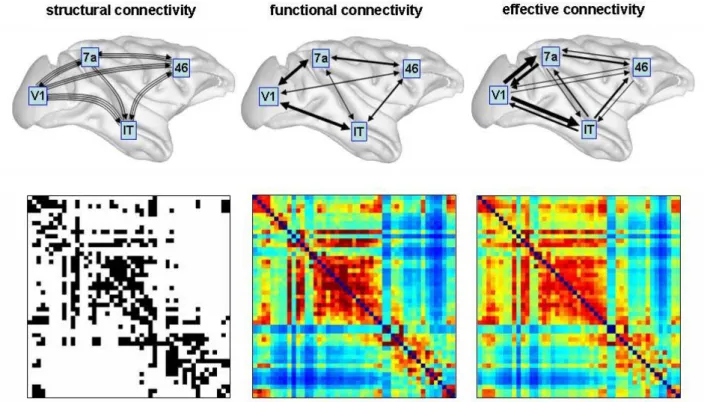
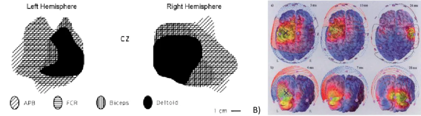
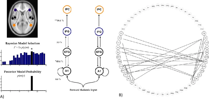
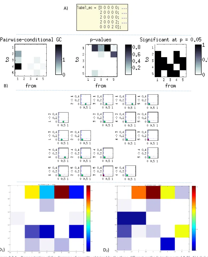
Figure 2.1-1 – Modes of brain connectivity. Top brain images illustrate structural connectivity (fiber pathways), functional connectivity (correlations), and effective connectivity (information flow) among four brain regions in macaque cortex, respectively. Matrices at the bottom show binary structural connections (left), symmetric mutual information (middle) and non-symmetric transfer entropy (right). (Honey et al. 2007). ... 19 Figure 2.2-1 – : Resting-state fMRI cerebral activity in 71 healthy subjects aged from19 to 80 years. Identification of the Default Mode Network (DMN). Adapted from Mevel et al. 2011. ... 20 Figure 2.2-2 – Schematic illustration how various methodological choices which might influence resting state data and, consequently, the construction of connectivity networks. Note that choice of connectivity measures is highly depended on methodological choices. The analysis should be split in two steps: Data selection and Connectivity measures. Adapted from Diessen, 2014 ... 21 Figure 2.3-1 – A) Action potential (left) and Postsynaptic potential (right). B) Pyramidal cells. C) Example of EEG signals, adapt from http://www.cs.sfu.ca/~hamarneh/340.html ... 22 Figure 2.4-1 – Exemple of an average of two conditions MEPs in a specific time window (ms) where the stimulus is applied. Adapted from Tomasevic et al. 2014. ... 24 Figure 2.4-2 – A) Direction of current flows in a magnetic coil and the induced current in the brain in (Hallett 2007). B) Schematic draw of stimulation with a figure-of-eight coil in cerebral cortex (scalp), in viewzone.com/tra nscranial.pro.jpg. ... 25 Figure 2.4-3 – A) The strength of the electric field induced in a spherical volume conductor below a circular (left) and a figure-of-eight coil (right), in (Illmoniemi et al. 1999). B) The comparison between the electric field created by two different coils, with a circular coil, and with a figure-of-eight coil (two circular coils), in (Nollet et al. 2003). ... 25 Figure 2.4-4 – A) TMS Mapping of Upper Extremity Muscles in Right and Left Sides of One Normal Subject after Stimulation of Contralateral M1s, in (Wassermann et al. 1992). B) Activation maps based on TMS-evoked averaged EEG responses, in (Ilmoniemi et al. 1997). ... 26 Figure 2.4-5 – Relative phase prior to and following TMS. Intensity levels are in radiants. (a) Max. Relative phase: pre-TMS. (b) Max. relative phase at the end of 5 min of single-pulse TMS. (c) Max. relative phase at the end of 25 min of single-pulse TMS. The relative phase increased almost uniformly across channels, though fronto-central/central and parietal channels had slightly higher relative phase changes, 25min after the start of TMS. Other variations appeared random. Although prior to or at the beginning of the TMS session clusters of channels had either positive or negative relative phases, indicating both spatial correlation/synchrony and de-correlation, at the end of the TMS session, almost all channels had positive relative phases, indicating correlation/synchrony Adapted from (Stamoulis et al. 2011). ... 27 Figure 2.5-1 – Visual comparison between a testing hypothesis model ( A) – DCM ) vs an exploratory model ( B) – GC ). A) (on left) Anatomical architecture of the DCM that best explains the brain responses. Such bilateral network has the highest log-evidence (on right) Network graph showing percentage changes in effective connectivity, Adapted from Dietz et al 2014, B) Directed graph representation of the significant interactions (in comparison to a control interval) at the P3 component between 322 and 410 ms using 24 electrodes. Adapted from Milde et al 2010... 33 Figure 3.2-1 – Demonstration of the diagrams of causality obtain by the three different methods implemented B-D). A) Label of true causalities (represented by a number ‘2’). B) Granger Causality
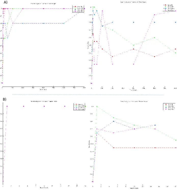
Page 14 of 89 Index. C) Factor Modelling in combination with Granger Causality Index. D1) Transfer Entropy (Non-Uniform embedding with binning estimator). D2) Transfer Entropy (Non-Uniform embedding with nearest neighbor estimator). In B) the left plot shows the values for GCI ‘from’ channels in the columns ‘to’ channels in the lines. The middle plot represent the respective p-values for the GCI, and finally in the right plot it is represented the statistical significant values for the GCI. In C) there is a figure with 20 subplots. Each one of them represent the causality ‘from’ channels in columns ‘towards’ channels in lines. In the x-axes it is represented the value for the determinant of the latent variables (see Annex 2), and in the y-axes it is represented the p-value for the F-test (H0: Ãij(m) = 0 for all m). The circles plotted in turquoise define causal relations, whereas the circles in red do not define causal relations. For both figures D) there is a representation of the TE values averaged across trials, where the colors define the magnitude of those values. The interpretation for these plot is that channels in the lines ‘cause’ channels in columns. All of these results are made over the simulated data (mentioned in the text) and have 2000 data points and here they are averaged over 10 trials/subjects. ... 36 Figure 3.2-2 – A) Variation of Sensitive (left) and Specificity (right) over length of data (x-axis), with the number of trials fixed (number of trials = 1) for the four methods: FM-GCI (red), GCI (green), TE with Binning Estimator (blue) and with Nearest-Neighbor (cyan). B) Variation of Sensitive (left) and Specificity (right) over number of trials (x-axis), with the length of data fixed (data points = 512), for the four methods: FM-GCI (red), GCI (green), TE with Binning Estimator (blue) and with Nearest-Neighbor (cyan). ... 37 Figure 3.3-1 – Histogram representation of the number of non-stationary channels present on the data per number of trials, given by the ADF statistical criterion (left side of each subplot) and by KPSS (right side of each subplot). On A) and B) the results are shown for the time-invariant data, with and without Non-stationary correction (see 3.3.1) respectively. On C) and D) the results are shown for the time-varying data, with and without Non-stationary correction. Inside the title brackets of each one of the histograms, there are the total number of channels that fail to show stationarity. ... 42 Figure 3.3-3 – Variation of Sensitive (left) and Specificity (right) over the number of ensemble trials for the time-invariant and time-varying, simulated data. ... 43 Figure 3.3-2 – Average over 200 trials of GC results for the time-invariant simulated data without and with Non-stationary correction, A) and B) respectively. GC results for the time-varying simulated data without and with Non-stationary correction, C) and D) respectively. E) Label of true causalities for the time-varying data (represented by a number ‘2’). For an interpretation of each of the different subplots see Figure 3.2-1. ... 43 Figure 3.4-1 – ERP simulated EEG data. Based on http://www.cs.bris.ac.uk/~rafal/phasereset/ ... 45 Figure 3.4-2 – A) Evolution of correlation coefficient over the increase of number of channels. B) Evolution of the maximum GCI value and the different between the maximum and the minimum GCI value, over the increase of number of channels. ... 46 Figure 3.4-3 – Correlations matrix across all channels for simulated EEG data with the following number of channels, n=5, n=10, n= 15, n=20, n=25, n=30. The closer the value to 1 (white), the more correlated are those two channels. The diagonal shows the correlations between the same channels, leading to a correlation of 1. ... 46 Figure 4.2-1 – Scheme of the experiment design. Each red bar represent the TMS stimulation which is followed by an TEP. Afterwards it is shown the resting state period which is the period of interest. These trials are repeated around 200 times. For both conditions the layout was similar. ... 49 Figure 4.2-2 – A) Experimental recording of TMS-EEG data. B) Schematic representation of the different stimulation hotspot – right superior parietal gyrus (depicted in red) and conditions optimal
Page 15 of 89 orientation (blue) and somato-auditory sham (pink). For the sham condition, a representation of the setup (bipolar electrical cutaneous stimulation (Oja 2006), coil placed on top of the electrical stimulation device placed over the hotspot. A total of 200 pulses was applied for each condition. 50 Figure 4.2-3 – Scheme of ECt toolbox architecture. ... 51 Figure 4.2-4 – A) Data plotted across all trials on only one channel, in green it is represented the triggers of the dataset. B) Data plotted across all trials for all-time-series in the 63 channels. C) Represents the contribution of each frequency to the PSD. Where it can be seen a huge movement in the alpha boundaries. The bold green line show the miss-behavior of the channel removed. On the yy axes in A) & B) it is shown the amplitude of the EEG (mV). ... 52 Figure 4.2-5 – itterative result over the AIC(p) – blue and BIC(p) – green, by selecting a model order (p) from 1 to 25. The minimum valeu will define the most suitable model order. The model order variaed across subject betwen p=9 and p=13. ... 53 Figure 4.3-1 – A) Matrix of Cross-Correlation between all channels of one subject after the preprocessing. B) Plot showing each model ‘consistency’ for the VAR model obtain at each set of trials (each red dot), for one subject, one condition. C) Percentage of the trials kept in the model per subject per condition (each odd number is representing the real TMS stimulation and each even number is the sham condition of each subject) (Subj.1 – 1,2; Subj.2 – 3,4; Subj.3 – 5,6; Subj.4 – 7,8; Subj.5 – 9,10; Subj.6 – 11,12). ... 56 Figure 4.3-2 – Granger Causality Index statistical analysis for one subject over the network, for the first level analysis. The information flow from the source in the column to the source in the line is coded by ’hot’ colours, an information flow from the source in the ’line’ to the source in the ’column’ is coded by an ’cold’ colour. Both matrixes are antisymmetric. The figure A) and B) show the z-score statistics over the paired t-test, corrected by FWR (Bonferroni correction), for condition rs on real TMS stimulation and condition rs on sham TMS stimulation, respectively, against a surrogate distribution RGT. ... 57 Figure 4.3-3 – A) Results of the 2nd Level Analysis of one subject. The information flow from the source in the column to the source in the line is coded by ’hot’ colours, an information flow from the source in the ’line’ to the source in the ’column’ is coded by an ’cold’ colour. This matrix is antisymmetric. B) Histogram of a 1000 permutation of the null-distribution on the maximal permutation statistics of a shuffle of both of the two condition. In green, it is represented the 95%-percentil that is used as threshold for relevance of the difference between condition rs on real TMS stimulation and rs on sham TMS stimulation, seen in A). The color bar it has arbitrary units since is the real difference of the GC values. The results for the other subjects can be seen in Figure A-0-7. ... 58 Figure 4.3-4 – Schematic map of information flow over independent components for one subject, over the second level analysis. The arrows width is proportional to the strength of the connections. The color bar it has arbitrary units since is the real difference of the GC values. The colors on the arrows are based on the matrix of the previous figure. ... 59
Figure 4.3-5 – Plots for the 3rd level Analysis. A) Matrix of the z-scores without FWE correction, showing the differences between all subjects of condition - real TMS, against conditon - sham TMS. The information flow from the source in the column to the source in the line is coded by ’hot’ colours, an information flow from the source in the ’line’ to the source in the ’column’ is coded by an ’cold’ colour, where basicly it inverts the caption in the plot. Another aspect, its the fact that this matrix is antisymmetric B) Represent the mask over the z-scores matrix showing the significance values over the z-score matrix without a FWE correction. Where ’0’ represent a significant connections, and ’1’ represents a non-significant connections. C) Results of p-values across all the causal connections after a FWE. ... 60
Page 16 of 89 Figures from Annex
Figure A-0-1 – TE values versus the number of significant realizations on a non-linear simulated
system. For the NUE and UE with LIN, BIN and NN, in (Montalto, Faes, and Marinazzo 2014). ... iii
Figure A-0-2 – The parameters of the strength of directed influence: b(n) denotes the strength of the influence bewtween y1 and y2, c(n) that between y3 and y1. In the xx axyes it is represented the data point ’n’, and in the yy axes its amplitude ... vi
Figure A-0-3 – Scheme of Stage 1 of ECt Toolbox – Preprocessing of the Data. ... vii
Figure A-0-4 – Scheme of Stage 2 of ECt Toolbox – Granger Causality Analysis ... viii
Figure A-0-5 – Scheme of stage 3 of ECt toolbox – Statistical Inference. ... ix
Figure A-0-6 – A) Power spectrum densities of the ICA components for the all concatenated time-series. B) Topoplots with the maps of the ICA components for the all concatenated time-time-series. This two outputs allow the visual checking for the most relevant independent components present in the time-series. ... x
Figure A- 0-7 –On the left side it is possible to see the results of the 2nd Level Analysis of 5 out of 6 subjects. Subject 1 shows a activity of 3.57% of the possible combinations, Subject 2 – 2.68%, Subject 4 – 8.93%, Subject 5 – 13.39%, Subject 6 - 0.89%. This percentage is obtain throw the following formula: (numb_channelActive / (numb_ channelsTotal * numb _ channelsTotal – numb_ channelsTotal) ) *100. The information flow from the source in the collumn to the source in the line is coded by ’summer’ colours, an information flow from the source in the line to the source in the collumn is coded by an ’winter’ colour. Each of the subject has to plots as in Figure 4.3-1.On the rigth side it is possible to see the histogram of a 1000 permutation of the null-distribution on the maximal permutation statistics of a shuffle of both of the two condition. In green, it is represented the 95%-percentile that is used as threshold for relevance of the difference between condition rs on real TMS stimulation and rs on sham TMS stimulation, seen in the respective plot. ... xii
Figure A-0-8 – Representation of the topographic maps plotting the independent components (Ics) that represent cortical responses... xiii
Page 17 of 89 Chapter 1
1. Motivation
The human brain is a fundamental part of the human being especially in the coordination of the sensory, cognitive and resting functions. Many studies in neuroscience have aimed to determine the brain activity for a particular task (Jirsa 2007) or associated to a specific disease (Nejad et al. 2012). What these studies report is that the brain runs in a highly dynamical and complex way, connecting different structures within itself. This brain connectivity is a broad concept that can be generally divided into three categories: structural, functional and effective connectivity. The structural connectivity refers to the connections of brain regions via nerve fibers. The functional connectivity deals with the temporal interdependencies among the activity of brain regions. The effective connectivity characterizes the causal (directed) effects among brain regions.
Trying to understand the complexity of neural networks lead neuroscientists to build paradigms where brain states could be deliberately modified. This can be achieved by measuring brain activity over cognition/somatosensory related task (Vetter, Smith, and Muckli 2014; Wu et al. 2014), where a network is activated over the specificity of the task, or by modelling the brain activity over external stimulation (Transcranial Magnetic Stimulation – TMS, Transcranial direct-current stimulation – tDCS) (Nollet et al. 2003). Such non-invasive techniques are based on the depolarization of neuronal populations of the underlying cortical area where a coil (TMS) or electrodes (tDCS) are placed, as well as of functional activation of connected areas via cortico-cortical interactions. These methods are more relevant regarding studies of effective connectivity of cortico-cortical interactions once they are independent from human control over the networks activation/deactivations.
When TMS is used in combination with electroencephalography (EEG), the direct effect on the electrical responses of those neurons to the TMS pulse can be observed as TMS-evoked potentials (TEPs). Even though they are specific from each area undergoing stimulation (latencies and number of components), they can be recorded in brain areas which are far away from the stimulation point. This gives TMS-EEG a powerful advantage in the study of effective connectivity, due to its geographical distribution and type of data. Some studies have looked into the direct cortical effect of TMS comparing different groups of participants (i.e. healthy controls and patients suffering from disorders of consciousness) (Rosanova et al. 2012; Ragazzoni et al. 2013; Ferrarelli et al. 2010), looking for different patterns of effective connectivity. However, two major limitations of these studies can be pointed out. Firstly, the methods used yet can not reveal the propagation path of the TMS-induced cortical activation in the EEG response. Secondly, associated with TMS stimulation, the pulse discharge also generates both a somatosensory scalp response and a loud “click” sound which induces in the EEG measurement somatosensory-evoked (SEPs) and auditory-evoked potentials (AEPs). Both of SEPs and AEPs are not a result of direct cortical activation, on that sense they will distort the TEPs and consequently the way cortical activation is measured.
Regarding the first issue, this project will apply a new approach of effective connectivity in TMS-EEG data, using Granger Causality (GC) (Granger 1969). According to the Wiener Causality concept (Wiener 1956), if adding the past and present information of a system X to the past and present information of a system Y improves predicting the future state of system Y, it can be concluded that X is the cause of Y. Some years later, that concept was limited in its general definition to linear bivariate autoregressive models and also translated in a mathematical formulation for quantitative inferences by (Granger 1969) originating the
Page 18 of 89 Granger Causality (GC). In 1982, Geweke proposed the most practical GC-based effective connectivity measure known as Granger Causality Index (GCI) (Geweke 1982). With it, it was also possible to build a tool that could distinguish correctly between direct and indirect causal links (Conditional Granger Causality Index (CGCI)) in the time domain (Ding M, Chen Y 2007), and the Direct Transfer Function (DTF), the Partial Direct Coherence (PDC) (Sameshima and Baccala 2001) and the Directed Direct Transfer Function (dDTF) in the frequency domain, where all are based on linear Multivariate Auto-Regressive (MVAR) models. The new combination that this project is aiming for is TMS-EEG with CGCI in the time-domain. On one hand CGCI will enable the track of information flow paths among nodes. On the other hand, TMS-EEG is a procedure that combines TMS with EEG, facilitating the location of the starting point in signal propagation, due to the TMS stimulation, that is then recorded by the EEG system. All together it forms a powerful tool in causality over conditioned brain states.
Accounting for the second issue, until now very few studies account for the influence of SEPs and AEPs in the seen results, and those who did used either conventional sham stimulation (only accounting for the AEPs) or a separate condition exploring SEPs with median nerve stimulation paradigms (Zanon et al. 2013). The use of conventional sham stimulation, moreover, does not result in a perceivable somatosentation due to a physical separation of the TMS coil from the scalp. The project proposal for that is to combined both influences and evaluate the remote evoked EEG responses derived from the target “behaviorally silent” scalp areas where TMS is commonly applied (i.e. parietal cortex), with the aim to generate resting state (rs) responses that match the multisensory components1 present in real TMS stimulation. Such protocol is intended to explore to which extent the effective connectivity tool here proposed is reliable. This is due to the fact that sham and real condition effect over the effective connectivity should be theoretically similar on the so-called resting state period in between the TMS pulses.
The main aim of this master thesis project is to combine a method for effective connectivity that gives “causality” and directionality (GC) with a brain controlled stimulation (TMS-EEG) in one powerful tool (a Matlab toolbox) to be used further to map the brain networks. The work is structured in two main steps. The first one is related with a methodological approach, where it is provided to the reader answers on why was GC used and how did the project account for the GC limitations based on simulated data (i.e. Non-stationarity and Colinearity). The second step is related to applying GC to TMS-EEG data, and then compare different conditions (i.e. Real-TMS vs Sham-TMS) trying to obtain significant results that help validating such tool. This will be achieved if the theoretical point of view on the resting states between different TMS stimulation procedures is seen in the results. This step accounts for the innovative approach on measuring the sham condition of TMS. Hopefully this thesis will be a first step on future developments on how can influences after a TMS pulse be measured.
Page 19 of 89 Chapter 2
2. Background
2.1. Brain Connectivity & Effective Connectivity
A complex system like the human body, could only be controlled and organized by a system that had a similar or higher order of complexity. That system is the Human Brain. Among all of that complexity, some things that have been concerning neuroscientists are (Swanson, 2003): How are brain areas connected? How is information going around the brain? And in which circumstances those connections happen? All of this merge towards asking how neurons and neural networks process information? And what is Brain Connectivity?
Brain connectivity refers to a pattern of anatomical links ("anatomical connectivity"), of statistical dependencies ("functional connectivity") or of causal interactions ("effective connectivity") between distinct units within a nervous system. The units correspond to individual neurons, neuronal populations, or anatomically segregated brain regions. Neural activity, and by extension neural codes, are constrained by connectivity. This patterns can be formed by structural links such as synapses or fiber pathways, or by statistical or causal relationships measured as cross-correlations, coherence, or information flow (Granger Causality or Dynamic Causal Models). Formally, brain connectivity patterns can be represented in graph or matrix format, see Figure 2.1-1. Structural brain connectivity forms a sparse and directed graph. Functional
Figure 2.1-1 – Modes of brain connectivity. Top brain images illustrate structural connectivity (fiber pathways), functional connectivity
(correlations), and effective connectivity (information flow) among four brain regions in macaque cortex, respectively. Matrices at the bottom show binary structural connections (left), symmetric mutual information (middle) and non-symmetric transfer entropy (right). (Honey et al. 2007).
Page 20 of 89 brain connectivity forms a full symmetric matrix, with each of the elements encoding statistically dependence among neurons, recording sites or voxels. Such matrices may be thresholded to yield binary undirected graphs, with the setting of the threshold controlling the degree of sparsity. Effective brain connectivity yields a full non-symmetric matrix inferring something on the directionality. This method attempts to extract networks of causal influences of one neural element over another (Valdes-Sosa et al. 2011). Reviews about the concept of connectivity, particularly in reference to effective connectivity, can be found in (Chicharro and Panzeri 2014; Valdes-Sosa et al. 2011). The interest of this can be related to network analysis techniques that allow the comparison of brain connectivity patterns, by using time-series data (e.g. TMS-EEG) where, by controlling the conditions of comparison, it would be possible to infer connectivity influences over different brain regions. Such issue will be the main line of this thesis2.
This chapter will be used to give an overview of the background needed for this project. A logical path is built such that the reader can understand fully the content of this thesis. This will include a first approach on a summary on resting state brain networks, EEG, TMS and TMS-EEG. Afterwards an introduction on the principles for Brain connectivity estimators and Granger Causality will be made, mentioning pros and cons. It is going to be finished with a short sum up of what have been done in this field.
2.2. Resting state brain network
In recent years, there has been a growing interest in characterizing the functional network of the brain ‘at rest’. This so-called ‘resting state’ (rs) paradigm is believed to reflect intrinsic activity of the brain, which may reveal valuable information on how different brain areas communicate, while the subject is not performing an explicit task. It gathers a variety of information, since it linked spontaneous – task independent – fluctuations in neural activity to diseases, cognitive decline, and disturbances in consciousness (van Diessen et al. 2015). Even though the interest in the ‘resting state’ has been associated with breakthroughs in functional magnetic resonance imaging (fMRI), such technique only provides an indirect measurement of brain activity and has a limited temporal resolution, e.g. Figure 2.2-1. Considering that part of the information processed in the brain at rest is encoded on time scales from milliseconds to seconds, a time scale that better suits techniques such as electroencephalography (EEG) and magnetoencephalography (MEG). EEG have been providing valuable information on deviant organization in the diseased brain, such as in Alzheimer’s disease, epilepsy, schizophrenia, multiple sclerosis, Parkinson’s disease, as well as in the healthy brain on topics as aging, gender differences and a healthy lifestyle, see (van Diessen et al. 2015) for a review.
2 Especially in the analysis between real TMS condition vs sham TMS condition.
Figure 2.2-1 – : Resting-state fMRI cerebral activity in 71 healthy subjects aged from19 to 80 years. Identification of the Default Mode
Page 21 of 89
‘Resting state’ per se
Resting state (rs) is the state in which a subject is awake and not performing an explicit mental or physical task. Initially, the ‘resting state’ condition was commonly used in EEG research – besides event-related potential studies – to study patterns of brain activity. The early EEG studies, including the first EEG recordings performed by Berger in 1929, already shown such patterns of brain activity. However, ironically it was when Biswal and colleagues revealed a distinct fMRI pattern of interacting brain regions when not performing a task that the resting state condition became a research paradigm for the study of interconnectivity of brain regions (Biswal et al. 1995). Since then, many studies have identified sets of brain regions that share a common activation pattern during the resting state including the ‘default mode network’3 and other so-called ‘resting state networks’4. These resting state networks have been replicated and validated both in neuroimaging and neurophysiological studies, suggesting that resting state patterns of connectivity are the result of robust and specific intrinsic neural activity (van Diessen et al. 2015).
Methodological concerns
When performing a rs study, especially when performing connectivity measures, there are some aspects that should be taken into account. There are three distinct issues: the subject-related methodological issues, the analysis-related methodological choices and the connectivity measures used.
Firstly, performing a resting state might not be as straightforward as it seems; behavior during the experiment and the perception of a stimulus independent from the condition may vary greatly between
3 Default Mode Network (DMN) - it is a network of brain regions that are active when the individual is not focused on
the outside world and the brain is at wakeful rest. Also called the default network, default state network, or task-negative network, the DMN is characterized by coherent neuronal oscillations at a rate lower than 0.1 Hz (one every ten seconds) (Fair et al. 2009).
4 Resting state networks (rsfMRI or R-fMRI) - is a method of functional brain imaging that can be used to evaluate
regional interactions that occur when a subject is not performing an explicit task. This resting brain activity is observed through changes in blood flow in the brain which creates what is referred to as a blood-oxygen-level dependent (BOLD) signal that can be measured using fMRI (Buckner 2013).
Figure 2.2-2 – Schematic illustration on how various methodological choices which might influence resting state data and,
consequently, the construction of connectivity networks. Note that choice of connectivity measures is highly depended on methodological choices. The analysis should be split in two steps: Data selection and Connectivity measures. Adapted from Diessen,
Page 22 of 89 subjects despite similar instructions. This variations can be in terms of state of vigilance (constantly shifting between different levels of activation, leading to differences in spectral power and functional connectivity), eyes open vs eyes closed and external induced heterogeneity (van Diessen et al. 2015). All these effects need to be taken into account. Secondly, the measurement-related methodological issues should be taken carefully. In Figure 2.2-2, the reader can find a summary of such issues. Diessen also suggested ’[...] Since the current literature is too diverse to provide an uniform methodological guideline, we suggest including different methodological approaches in resting state studies to better understand the influence of these approaches on study results’, an aspect that is going to be discussed in chapter 3 – Managing Granger Causality over EEG signals. Finally accounting for the influence of the connectivity measures chosen, (van Diessen et al. 2015), provides a good review stating that caution should be taken, regarding that some connectivity measures are more vulnerable to volume conduction5, which leads to unreliable connectivity values, and consequently, unreliable network estimations.
2.3. Electroencephalography - EEG
The brain generates electric current/charge that is maintained by billions of neurons. They are polarized by membrane transport proteins that pump ions across their membranes, a process that occurs constantly. These exchanges lead to periods when the neuron is in a resting potential or periods where there are a propagation of action potentials. The signal propagation can be yield by cascade phenomenon. Everything happens due to ions chain, where when ions of similar charge repel each other, they tend to push their neighbors, which then push their neighbors, leading to a wave of propagation. This is known as volume conduction, and as the reader will see ahead, is also one of the EEG drawbacks on Effective Connectivity. In order to measure those waves of propagation, it is necessary for the ions to reach the electrodes on the scalp, and then ions will start the cascade of dragging more ions and so forward (Tatum, W. O. et al. 2008).
The electric activity in the cortex has two components, the action potential and the excitatory postsynaptic potential (EPSP), see Figure 2.3-1 A). The action potential is presynaptic, axonal and generally
5 Volume Conduction – is the propagation of electromagnetic field with a speed of light — 3⋅1010 cm/s. For the distance
of the order of centimeter the delay is roughly 3.3⋅10−9 s. Such delay cannot be practically detected, and affect/smears
the information of each EEG sensor (Broek et al. 1998).
Figure 2.3-1 – A) Action potential (left) and Postsynaptic potential (right). B) Pyramidal cells. C) Example of EEG signals, adapt from http://www.cs.sfu.ca/~hamarneh/340.html
B)
C)
Page 23 of 89 not-measurable by EEG, on the other hand the EPSP is postsynaptic, dendritic and it is measurable with EEG. However, the electric potential generated by an individual neuron is far too small to be picked up by EEG - Figure 2.3-1 C). EEG activity therefore always reflects the summation of the synchronous activity of thousands or millions of neurons that have similar spatial orientation. If the cells do not have similar spatial orientation, their ions do not line up and consequently waves created in this way are not detected. Pyramidal neurons (Figure 2.3-1 B)), which are oriented tangentially to the scalp surface of the cortex are thought to produce the most EEG signal because they are well-aligned and fire together. Moreover, the scalp EEG activity shows oscillations at a variety of frequencies. Among them, there are Delta waves (up to 4 Hz), Theta waves (4Hz-7Hz), Alpha waves (7-14Hz), Beta waves (15Hz-30) and finally Gamma waves (above 32Hz) (Nunez PL et al. 1981).
All of these waves are known as brainwaves and they codify thoughts, emotions and behaviors, being dependent over the task, stimulation or behavioral situation to which the subject is insert. They work together in the sense that, in the brain there is a coupling of different brainwaves. Such coupling can be constraint to a specific brain area or can be much wider, according to the task specificity (Canolty et al. 2009). With this being said, frequency bands that represent brainwaves are much related with the understanding of the brain functions and connections. Many studies have been pointing out the relevance of these brainwaves, showing measures for coherence, cross-coupling frequencies among others, trying to infer over the brain paths of communications. However, in this thesis the specificity of the frequency will not be in focus, since the effective connectivity will be performed on the time-domain.
On the practical point of view, one thing that should be kept in mind is that, the signal recorded is affected by biological and external artifacts. To try to reduce those issues and obtain a noise free signal some considerations should be taken into account. Firstly, the signal has to be measured over the scalp with surface electrodes (made of AgCl) that maintain a very constant potential, and have high capacity. However, due to a very small amplitude, it is necessary to amplify it, in order to have a reasonable output. Secondly, it is necessary to reference the signal, which can be made by one of the three possibilities: reference electrode, average reference and Laplacian montage. Thirdly, EEG electrical signal detected along the scalp is much affected by biological artifacts with different amplitudes, such as eye-induced artifacts and / or muscle activation. There are also more artifacts, such as environmental artifacts that are mostly created by the surrounding environment of the recording process. Important to mention is also the problem of volume conduction, on the scalp which if not controlled for, will lead to smeared EEG information. However, we are going to discuss on how to solve this problem in section 3.4.3 and section 4.2, due to the challenging procedureof the pre-processing for effective connectivity, an acceptable answer is by solving the inverse problem. In order words by converting the sensor space into the source space.
Sensor space to source space
Understanding brain function requires sophisticated methods applicable to non-invasively measured bioelectric signals (EEG data). Those methods should avoid, as well as possible the contamination by artifacts or any type of perturbation that diminish the quality and veracity of the information. It was with this in mind, that the neuroscience community started to look into a different level of analysis, shifting the attention from the sensor space (where the EEG signal is recorded) to a cortical level. This is the so-called source level, and it tries to translate the dataset recorded over the localization of the brain sources beyond it, giving the activity over time for those sources. However, to achieve that is necessary to solve the inverse problem.
Page 24 of 89 The source localization procedure works by first finding the scalp potentials that would result from hypothetical dipoles, or more generally from a current distribution inside the head – the forward problem, see Figure 2.3-2. Then, in conjunction with the actual EEG data measured at specified positions of (usually less than 100) electrodes on the scalp, it can be used to work back and estimate the sources that fit these measurements – the inverse problem. The accuracy with which a source can be located is affected by a number of factors including head-modelling errors, source-modelling errors and EEG noise (instrumental or biological). The two main categories of methods which were developed to solve the EEG inverse problem are mainly the parametric and the non-parametric methods. The main difference between the two is whether a fixed number of dipoles is assumed a priori or not, respectively. This is out of the scope of this thesis, nevertheless a review can be found in (Grech et al. 2008).
2.4. Transcranial Magnetic Stimulation - TMS
2.4.1. Physics and Biophysics of TMSElectromagnetic induction, i.e., the induction of an electrical current in a circuit exposed to a changing field, is an old concept firstly introduced by Faraday in 1831:
𝜀 =∆𝛷𝐵
∆𝑡, where 𝛷𝐵 = ∫ 𝐵 ∙ 𝑑𝑆𝑆 Equation 2.4-1
Figure 2.4-1 – Exemple of an average of two conditions MEPs in a specific time window (ms) where the stimulus is applied. Adapted from Tomasevic et al. 2014.
Figura 2.3-2 - A three layer head model. In symbolic terms, the EEG forward problem is that of finding, in a reasonable time, the
potential g(r, rdip, d) at an electrode positioned on the scalp at a point having position vector r due to a single dipole with dipole
Page 25 of 89 Connecting this principle with what was said above regarding electric brain activity, it could be hypothesized that it is possible to apply it in the human brain. The motor evoked potential (MEP – see Figure 2.4-1) comprises the proof of that concept. To obtain an MEP, a stimulus with a magnetic coil over the motor cortex is applied, and due to the central nervous system pathways, it is possible to induce a response in the peripheral muscles given an enough intensity of stimulation. The first approach using the electromagnetic induction principle to non-invasively stimulate the brain was made by Barker (Barker et al. 1985).
Basic physics principles
TMS creates a pulsed electric current induced by the time-varying magnetic field that can depolarize neurons. Although the actual pathways being investigated are not known, they incorporate the fastest conducting fibers which might include the pyramidal tracts (Corthout et al 2001). A magnetic field is generated by passing an electric current through a coil of wire, called magnetic coil – Figure 2.4-2 A), which is placed above the scalp – Figure 2.4-2 B). Due to Faraday Law, the magnetic pulse produced from a perpendicular electric current pulse will thus induce a current in an electrically conductive region (e.g. human brain). This current will be in intensity proportional to the magnetic field (Nollet et al. 2003), and can only be produced because the skull presents a low impedance to magnetic fields of this frequency. Flux lines around the coil represent the magnetic field and it is measured in Tesla (T).
In an homogenous medium, the magnetic field will induce, as can be seen in Figure 2.4-2 A), a parallel current that flows only parallel to the plane of the coil. There would be a difference in the tissues interaction with the magnetic field, according to the position relative to the coil. The loops near the coil will have a
B)
Figure 2.4-2 – A) Direction of current flows in a magnetic coil and the induced current in the brain in (Hallett 2007). B) Schematic draw
of stimulation with a figure-of-eight coil in cerebral cortex (scalp), in viewzone.com/tra nscranial.pro.jpg.
A)
Figure 2.4-3 – A) The strength of the electric field induced in a spherical volume conductor below a circular (left) and a
figure-of-eight coil (right), in (Illmoniemi et al. 1999). B) The comparison between the electric field created by two different coils, with a circular coil, and with a figure-of-eight coil (two circular coils), in (Nollet et al. 2003).
B) A)
Page 26 of 89 stronger current, while with the distance the strength falls. Due to this, TMS is only able to stimulate areas in the brain in a depth of 1-2cm in the cortex (Hess et al. 1987).
Most related with the problem of deepness and focality, is the specificity of the coil. According to those is possible to obtain different results. In that sense, magnetic coils may have different shapes Figure 2.4-3 A). Circular coils (usually with diameter of 5-10cm) induce a more widespread, less focal activation, while figure-of-eight shaped coils are more focal, producing maximal current at the intersection of the two round components as it can clearly be seen in Figure 2.4-3. Nevertheless, these coils have a lower induction than circular coils (Hallett 2007).
Comparing this technique with transcranial electrical stimulation (TES), it has been concluded that TMS has some advantages. One of the most significative is that it is not painful. Another one is that the electrical field induced with a coil decreases significantly less with the increasing distance of the propagation in the brain than a field induced by TES. This is due to the fact that electrical stimulation injects current into the body via a surface, while magnetic stimulation uses a pulse of magnetic field to cause the voltage difference between two points, triggering a natural process. This leads to lesser loss of ions on the process of activation/inhibition pathways (Nollet et al. 2003).
Biophysical approach
Since TMS was introduced, there has been a debate over which structures are participating in the propagation of the stimulus. Now it is known that there are two types of waves that conduct the signals, the ones that produce a direct activation (D-waves) and the ones that produce an indirect activation (I-waves) of the corticospinal tract. The D-waves conduct down the pyramidal system, which can be activated trans-synaptically only at higher intensities. In contrast, the lower threshold form of TMS, for instance over the hand area of M1, tend to commonly activate corticospinal neurons trans-synaptically in the pyramidal tract which activates I-waves. However, with higher intensities, both D-waves and I-waves are activated (Di Lazzaro, et al. 1998).
Using TMS, the brain can be briefly activated or briefly inhibited; in fact, likely both occur with each stimulus in different amounts and with different time courses. Such effect can be used to localize brain functions in both space and time. Many studies have been conducted but of most interest are the approaches in the motor system, mainly due to its practicability throw the measures of the Motor Evoked Potential (MEP) in the peripheral nerve. One of them is the study of (Wassermann et al 1992), which concludes that body parts, such as arm and leg, are completely separate, but there is overlapping of muscles in the same body
Figure 2.4-4 – A) TMS Mapping of Upper Extremity Muscles in Right and Left Sides of One Normal Subject after Stimulation of
Contralateral M1s, in (Wassermann et al. 1992). B) Activation maps based on TMS-evoked averaged EEG responses, in (Ilmoniemi
et al. 1997).
Page 27 of 89 part, Figure 2.4-4 A). Such study was performed with single pulses of TMS6. However, many other protocols exist, e.g. repetitive TMS protocols (rTMS) and the paired-pulse TMS. As a final comment, there is an inter-MEP variability, which the reason is not yet known. It might be related to ongoing activity differences between TMS pulses. Thus, many trials should be performed in other to obtain a reliable conclusion on the data obtained.
Another aspect of most interest is the capability of specific TMS pulses to influence the behavior of the brain in the medium/long run, the so-called induced plasticity. Very briefly, neuroplasticity, also known as brain plasticity, encompasses both synaptic plasticity and non-synaptic plasticity—it refers to changes in neural pathways and synapses due to changes in behavior, environment or neural processes. Depending on the type of TMS pulse and the area of stimulation, this effect can be more or less prominent. Regarding the single-pulse paradigm used during this thesis, Pellicciari (Pellicciari et al. 2015) studied the effects of several single TMS pulses, delivered at two different inter-trial intervals, on corticospinal excitability. The author found that Motor Evoked Potential (MEPs) significantly increased when the TMS pulses were delivered at both random and fixed inter-trial intervals, leading them to conclude that single TMS pulses induce cumulative changes in neural activity during a single pulse TMS stimulation, resulting in a motor cortical excitability increase. However, as others studies have reported, such effects are only transient stimulation-related effects in the amplitude (or frequency domains) following single-pulse TMS. Stamoulis (Stamoulis et al. 2011) resented novel results of cumulative effects of single-pulse TMS, at least in terms of phase changes in the EEG in a small number of healthy subjects. Although the exact mechanism of phase modulation by TMS is unclear, the author presented evidence that such modulation exists and results from the prolonged but not short term application of single-pulse TMS applied in the motor cortex, see Figure 2.4-5. These studies support the idea that between a real-TMS and a sham-TMS in the short term there are no differences in the resting state, in between pulses, of the brain networks.
6 Single pulse TMS – is a pulse that occurs at a frequency over a time allowing for the recovery of rs in the brain.
Figure 2.4-5 – Relative phase prior to and following TMS. Intensity levels are in radiants. (a) Max. Relative phase: pre-TMS. (b) Max.
relative phase at the end of 5 min of single-pulse TMS. (c) Max. relative phase at the end of 25 min of single-pulse TMS. The relative phase increased almost uniformly across channels, though fronto-central/central and parietal channels had slightly higher relative phase changes, 25min after the start of TMS. Other variations appeared random. Although prior to or at the beginning of the TMS session clusters of channels had either positive or negative relative phases, indicating both spatial correlation/synchrony and de-correlation, at the end of the TMS session, almost all channels had positive relative phases, indicating correlation/synchrony.