EUROPEAN ORGANISATION FOR NUCLEAR RESEARCH (CERN)
Submitted to: JHEP
DOI:10.1007/JHEP10(2017)182
CERN-EP-2017-119 16th November 2017
Search for new high-mass phenomena in the
dilepton final state using 36 fb
−1
of proton–proton
collision data at
√
s
= 13 TeV with the ATLAS
detector
The ATLAS Collaboration
A search is conducted for new resonant and non-resonant high-mass phenomena in dielectron and dimuon final states. The search uses 36.1 fb−1of proton–proton collision data, collected
at √s = 13 TeV by the ATLAS experiment at the LHC in 2015 and 2016. No significant
deviation from the Standard Model prediction is observed. Upper limits at 95% credibility level are set on the cross-section times branching ratio for resonances decaying into dileptons, which are converted to lower limits on the resonance mass, up to 4.1 TeV for the E6-motivated Z0χ. Lower limits on the qq`` contact interaction scale are set between 24 TeV and 40 TeV, depending on the model.
c
2017 CERN for the benefit of the ATLAS Collaboration.
1 Introduction
This article presents a search for resonant and non-resonant new phenomena, based on the analysis of dilepton final states (ee and µµ) in proton–proton (pp) collisions with the ATLAS detector at the Large
Hadron Collider (LHC) operating at √s= 13 TeV. The data set was collected during 2015 and 2016, and
corresponds to an integrated luminosity of 36.1 fb−1. In the search for new physics carried out at hadron colliders, the study of dilepton final states provides excellent sensitivity to a large variety of phenomena. This experimental signature benefits from a fully reconstructed final state, high signal-selection efficien-cies and relatively small, well-understood backgrounds, representing a powerful test for a wide range of theories beyond the Standard Model (SM).
Models with extended gauge groups often feature additional U(1) symmetries with corresponding heavy spin-1 bosons. These bosons, generally referred to as Z0, would manifest as a narrow resonance through its decay, in the dilepton mass spectrum. Among these models are those inspired by Grand Unified Theories, which are motivated by gauge unification or a restoration of the left–right symmetry violated by the weak interaction. Examples considered in this article include the Z0bosons of the E6-motivated [1, 2] theories as well as Minimal models [3]. The Sequential Standard Model (SSM) [2] is also considered
due to its inherent simplicity and usefulness as a benchmark model. The SSM manifests a ZSSM0 boson
with couplings to fermions equal to those of the SM Z boson.
The most sensitive previous searches for a Z0 boson decaying into the dilepton final state were carried out by the ATLAS and CMS collaborations [4,5]. Using 3.2 fb−1of pp collision data at √s = 13 TeV collected in 2015, ATLAS set a lower exclusion limit at 95% credibility level (CL) on the Z0SSMpole mass of 3.4 TeV for the combined ee and µµ channels. Similar limits were set by CMS using the 2015 data sample.
This search is also sensitive to a series of other models that predict the presence of narrow dilepton
resonances. These models include the Randall–Sundrum (RS) model [6] with a warped extra dimension
giving rise to spin-2 graviton excitations, the quantum black-hole model [7], the Z∗model [8], and the minimal walking technicolour model [9]. In order to facilitate interpretation of the results in the context of these or any other model predicting a new dilepton resonance, limits are set on the production of a generic Z0-like excess.
In addition to the search for narrow resonances, results for non-resonant phenomena are also reported. Such models of these phenomena include an effective four-fermion contact interaction (CI) between two initial-state quarks and two final-state leptons (qq``). Unlike resonance models, which require sufficient energy to produce the new gauge boson, the presence of a new interaction in the non-resonant regime can be detected at a much lower energy.
The most stringent constraints from CI searches are also provided by the ATLAS and CMS collabora-tions [4, 10], for couplings between quarks and leptons. Using 3.2 fb−1 of pp collision data at √s =
13 TeV collected in 2015, ATLAS set lower limits on the qq`` CI scale ofΛ = 25 TeV and Λ = 18 TeV
at 95% CL for constructive and destructive interference, respectively, in the case of left–left interactions and assuming a uniform positive prior probability in 1/Λ2. Similar limits were set by CMS using the 2015 data set. Both the resonant and non-resonant models considered as the benchmark for this search are further discussed in Section2.
The presented search utilises the invariant mass spectra of the observed dilepton final states as discrim-inating variables. The analysis and interpretation of these spectra rely primarily on simulated samples of
signal and background processes. The interpretation is performed taking into account the expected shape of different signals in the dilepton mass distribution. The use of the shape of the full dilepton invariant mass distribution reduces the uncertainties in the background modelling, thereby increasing the sensitiv-ity of this search at high masses. This article is structured as follows: Section2 covers the theoretical motivation of the models considered in this search, followed by a description of the ATLAS detector in Section3, and a summary in Section4of the data and Monte Carlo (MC) samples used. The event selec-tion is motivated and described in Secselec-tion5, with details of the background estimation given in Section6, and an overview of the systematic uncertainty treatment given in Section7. The event yields and main kinematic distributions are presented in Section8, followed by a description of the statistical analysis in Section9, and the results in Section10.
2 Theoretical models
2.1 E6-motivated Z0 modelsIn the class of models based on the E6 gauge group [1,2], the unified symmetry group can break to the SM in a number of different ways. In many of them, E6is first broken to SO(10) × U(1)ψ, with SO(10) then breaking either to SU(4) × SU(2)L× SU(2)Ror SU(5) × U(1)χ. In the first of these two possibilities, a Z3R0 coming from SU(2)R, where 3R stands for the right-handed third component of weak isospin, or a ZB-L0 from the breaking of SU(4) into SU(3)C× U(1)B−L could exist at the TeV scale, where B (L) is the
baryon (lepton) number and (B − L) is the conserved quantum number. Both of these Z0 bosons appear
in the Minimal Z0 models discussed in the next section. In the SU(5) case, the presence of U(1)ψ and U(1)χsymmetries implies the existence of associated gauge bosons Zψ0 and Z0χthat can mix. When SU(5) is broken down to the SM, one of the U(1) can remain unbroken down to intermediate energy scales. Therefore, the precise model is governed by a mixing angle θE6, with the new potentially observable Z
0 boson defined by Z0(θE6) = Z
0
ψcos θE6 + Z
0
χsin θE6. The value of θE6 specifies the Z
0 boson’s coupling
strength to SM fermions as well as its intrinsic width. In comparison to the benchmark ZSSM0 , which has a width of approximately 3% of its mass, the E6models predict narrower Z0signals. The Zψ0 considered here has a width of 0.5% of its mass, and the Zχ0 has a width of 1.2% of its mass [11,12]. All other Z0 signals in this model, including ZS0, Z0I, Zη0, and ZN0, are defined by specific values of θE6 ranging from 0 to
π, and have widths between those of the Z0
ψ and Zχ0.
2.2 Minimal Z0 models
In the Minimal Z0 models [3], the phenomenology of Z0 boson production and decay is characterised
by three parameters: two effective coupling constants, gBL and gY, and the Z0 boson mass. This para-meterisation encompasses Z0 bosons from many models, including the Zχ0 belonging to the E6-motivated model of the previous section, the Z3R0 in a left-right symmetric model [13,14] and the ZB-L0 of the pure (B − L) model [15]. The minimal models are therefore particularly interesting for their generality, and because couplings are being directly constrained by the search. The coupling parameter gBL defines the coupling of a new Z0boson to the (B − L) current, while the gYparameter represents the coupling to the weak hypercharge Y. It is convenient to refer to the ratios ˜gBL ≡ gBL/gZ and ˜gY ≡ gY/gZ, where gZ is
related to the coupling of the SM Z boson to fermions defined by gZ = 2MZ/v. Here v = 246 GeV is
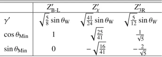
chosen as independent parameters with the following definitions: ˜gBL = γ0cos θMin, ˜gY= γ0sin θMin. The γ0 parameter measures the strength of the Z0 boson coupling relative to that of the SM Z boson, while θMindetermines the mixing between the generators of the (B − L) and weak hypercharge Y gauge groups. Specific values of γ0and θMincorrespond to Z0 bosons in various models, as is shown in Table1for the three cases mentioned in this section.
Table 1: Values for γ0and θMinin the Minimal Z0models corresponding to three specific Z0bosons: ZB-L0 , Zχ0 and
Z3R0 . The SM weak mixing angle is denoted by θW.
ZB-L0 Z0χ Z3R0 γ0 q5 8sin θW q 41 24sin θW q 5 12sin θW cos θMin 1 q 25 41 1 √ 5 sin θMin 0 − q 16 41 − 2 √ 5
For the Minimal Z0 models, the width depends on γ0 and θMin, and the Z0 interferes with the SM Z/γ∗ process. For example, taking the 3R and B − L models investigated in this search, the width varies from
less than 1% up to 12.8% and 39.5% respectively, for the γ0 range considered. The branching fraction
to leptons is the same as for the other Z0 models considered in this search. Couplings to hypothetical right-handed neutrinos, the Higgs boson, and to W boson pairs are not considered. Previous limits on the Z0mass versus γ0 were set by the ATLAS experiment. For γ0 = 0.2, the range of Z0 mass limits at 95% CL corresponding to θMin ∈ [0, π] is 1.11 TeV to 2.10 TeV [16].
2.3 Contact interactions
Some models of physics beyond the SM result in non-resonant deviations from the predicted SM dilepton mass spectrum. Compositeness models motivated by the repeated pattern of quark and lepton generations predict new interactions involving their constituents. These interactions may be represented as a contact interaction between initial-state quarks and final-state leptons [17, 18]. Other models producing non-resonant effects are models with large extra dimensions [19] motivated by the hierarchy problem. This search is sensitive to non-resonant new physics in these scenarios; however, constraints on these models are not evaluated in this article.
The following four-fermion CI Lagrangian [17,18] is used to describe a new interaction in the process qq →`+`−: L = g 2 Λ2 [ηLL(qLγµqL) (`Lγ µ` L)+ ηRR(qRγµqR) (`Rγµ`R) +ηLR(qLγµqL) (`Rγµ`R)+ ηRL(qRγµqR) (`Lγµ`L)] ,
where g is a coupling constant set to be √4π by convention, Λ is the CI scale, and qL,R and `L,R are
left-handed and right-handed quark and lepton fields, respectively. The symbol γµ denotes the gamma
matrices, and the parameters ηi j, where i and j are L or R (left or right), define the chiral structure of the new interaction. Different chiral structures are investigated here, with the left–right (right–left) model
obtained by setting ηLR = ±1 (ηRL = ±1) and all other parameters to zero. Likewise, the left–left and right–right models are obtained by setting the corresponding parameters to ±1, and the others to zero. The sign of ηi jdetermines whether the interference between the SM Drell–Yan (DY) qq → Z/γ∗→`+`− process and the CI process is constructive (ηi j = −1) or destructive (ηi j= +1).
3 ATLAS detector
The ATLAS experiment [20,21] at the LHC is a multipurpose particle detector with a forward-backward symmetric cylindrical geometry and a near 4π coverage in solid angle.1 It consists of an inner detector for tracking surrounded by a thin superconducting solenoid providing a 2 T axial magnetic field, elec-tromagnetic and hadronic calorimeters, and a muon spectrometer. The inner detector (ID) covers the pseudorapidity range |η| < 2.5. It consists of silicon pixel, silicon microstrip, and transition-radiation tracking detectors. Lead/liquid-argon (LAr) sampling calorimeters provide electromagnetic (EM) energy measurements with high granularity. A hadronic (steel/scintillator-tile) calorimeter covers the central pseudorapidity range (|η| < 1.7). The endcap and forward regions are instrumented with LAr calorimet-ers for EM and hadronic energy measurements up to |η|= 4.9. The total thickness of the EM calorimeter is more than twenty radiation lengths. The muon spectrometer (MS) surrounds the calorimeters and is based on three large superconducting air-core toroids with eight coils each. The field integral of the tor-oids ranges between 2.0 and 6.0 T m for most of the detector. The MS includes a system of precision tracking chambers and fast detectors for triggering. A dedicated trigger system is used to select events. The first-level trigger is implemented in hardware and uses the calorimeter and muon detectors to reduce the accepted rate to below 100 kHz. This is followed by a software-based trigger that reduces the accepted event rate to 1 kHz on average [22].
4 Data and Monte Carlo samples
This analysis uses data collected at the LHC during 2015 and 2016 pp collisions at √s= 13 TeV. The
total integrated luminosity corresponds to 36.1 fb−1, considering the periods of data-taking with all sub-detectors functioning nominally. The event quality is also checked to remove events which contain noise bursts or coherent noise in the calorimeters.
Modelling of the various background sources primarily relies on MC simulation. The dominant back-ground contribution arises from the DY process, which was simulated using the next-to-leading-order (NLO) Powheg Box [23] event generator, implementing the CT10 [24] parton distribution function (PDF), in conjunction with Pythia 8.186 [25] for event showering, and the ATLAS AZNLO set of tuned paramet-ers [26]. A more detailed description of this process is provided in Ref. [27]. The DY event yields are cor-rected with a rescaling that depends on the dilepton invariant mass from NLO to next-to-next-to-leading
order (NNLO) in the strong coupling constant, computed with VRAP 0.9 [28] and the CT14NNLO PDF
set [29]. The NNLO quantum chromodynamic (QCD) corrections are a factor of ∼ 0.98 at a dilepton
in-variant mass (m``) of 3 TeV. Mass-dependent electroweak (EW) corrections were computed at NLO with
1ATLAS uses a right-handed coordinate system with its origin at the nominal interaction point (IP) in the centre of the detector
and the z-axis along the beam pipe. The x-axis points from the IP to the centre of the LHC ring, and the y-axis points upwards. Cylindrical coordinates (r, φ) are used in the transverse plane, φ being the azimuthal angle around the z-axis. The pseudorapidity is defined in terms of the polar angle θ as η= − ln tan(θ/2). Angular distance is measured in units of ∆R ≡ p(∆η)2+ (∆φ)2.
Mcsanc 1.20 [30]. The NLO EW corrections are a factor of ∼ 0.86 at m``= 3 TeV. Those include photon-induced contributions (γγ → `` via t- and u-channel processes) computed with the MRST2004QED PDF set [31].
Other backgrounds originate from top-quark [32] and diboson (WW, WZ, ZZ) [33] production. The dibo-son processes were simulated using Sherpa 2.2.1 [34] with the CT10 PDF. The t¯t and single-top-quark MC samples were simulated using the Powheg Box generator with the CT10 PDF, and are normalised to a cross-section as calculated with the Top++ 2.0 program [35], which is accurate to NNLO in perturbative QCD, including resummation of next-to-next-to-leading logarithmic soft gluon terms. Background pro-cesses involving W and Z bosons decaying into τ lepton(s) were found to have a negligible contribution, and are not included. In the case of the dielectron channel, multi-jet and W+jets processes (which contrib-ute due to the misidentification of jets as electrons) are estimated using a data-driven method, described in Section6.
Signal processes were produced at leading-order (LO) using Pythia 8.186 with the NNPDF23LO PDF set [36] and the ATLAS A14 set of tuned parameters [37] for event generation, parton showering and
hadronisation. Interference effects (with DY production) are not included for the SSM and E6 model
Z0signal due to large model dependence, but are included for the CI signal and for the Minimal model approach. Higher-order QCD corrections for the signal were computed with the same methodology as for the DY background. EW corrections were not applied to the Z0signal samples also due to the large model dependence. However, the EW corrections are applied to the CI signal samples, because interference effects are included.
The detector response is simulated with Geant 4 [38], and the events are processed with the same re-construction software [39] as used for the data. Furthermore, the distribution of the number of additional simulated pp collisions in the same or neighbouring beam crossings (pile-up) is accounted for by
overlay-ing minimum-bias events simulated with Pythia 8.186 usoverlay-ing the ATLAS A2 set of tuned parameters [37]
and the MSTW2008LO PDF set [40], reweighting the MC simulation to match the distribution observed
in the data.
5 Event selection
Dilepton candidates are selected in the data and simulated events by requiring at least one pair of recon-structed same-flavour lepton candidates (electrons or muons) and at least one reconrecon-structed pp interaction vertex, with the primary vertex defined as the one with the highest sum of track transverse momenta (pT) squared.
Electron candidates are identified in the central region of the ATLAS detector (|η| < 2.47) by combining calorimetric and tracking information in a likelihood discriminant with four operating points: Very Loose, Loose, Medium and Tight each with progressively higher threshold for the discriminant, and stronger background rejection, as described in Ref. [41]. The transition region between the central and forward regions of the calorimeters, in the range 1.37 ≤|η| ≤ 1.52, exhibits poorer energy resolution and is there-fore excluded. Electron candidates are required to have transverse energy (ET) greater than 30 GeV, and a track consistent with the primary vertex both along the beamline and in the transverse plane. The Medium working point of the likelihood discrimination is used to select electron candidates while the Very Loose and Loose working points are used in the data-driven background estimation described in Section6. In addition to the likelihood discriminant, selection criteria based on track quality are applied. The selection
efficiency is approximately 96% for electrons with ET between 30 GeV and 500 GeV, and decreases to
approximately 95% for electrons with ET = 1.5 TeV. The selection efficiency is evaluated in the data
using a tag-and-probe method [42] up to ET of 500 GeV and the uncertainties due to the modelling of the shower shape variables are estimated for electrons with higher ETusing MC events, as described in Section7. The electron energy scale and resolution have been calibrated up to ET of 1 TeV using data collected at √s= 8 TeV and √s= 13 TeV [43]. The energy resolution extrapolated for high-ETelectrons (greater than 1 TeV) is approximately 1%.
Muon candidate tracks are, at first, reconstructed independently in the ID and the MS [44]. The two
tracks are then used as input to a combined fit (for pT less than 300 GeV) or to a statistical combination (for pT greater than 300 GeV). The combined fit takes into account the energy loss in the calorimeter and multiple-scattering effects. The statistical combination for high transverse momenta is performed to mitigate the effects of relative ID and MS misalignments.
In order to optimise momentum resolution, muon tracks are required to have at least three hits in each of three precision chambers in the MS and not to traverse regions of the MS which are poorly aligned. This requirement reduces the muon reconstruction efficiency by about 20% for muons with a pTgreater than 1.5 TeV. Furthermore, muon candidates in the overlap of the MS barrel and endcap region (1.01 < |η| < 1.10) are rejected due to the potential relative misalignment between barrel and endcap. Measure-ments of the ratio of charge to momentum (q/p) performed independently in the ID and MS must agree within seven standard deviations, calculated from the sum in quadrature of the ID and MS momentum uncertainties. Finally, in order to reject events that contain a muon with poor track resolution in the MS,
due to a low magnetic field integral and other effects, an event veto based on the MS track momentum
measurement uncertainty is also applied. Muons are required to have pTgreater than 30 GeV, |η| < 2.5, and to be consistent with the primary vertex both along the beamline and in the transverse plane.
To further suppress background from misidentified jets as well as from light-flavour and heavy-flavour hadron decays inside jets, lepton candidates are required to satisfy calorimeter-based (only for electrons) and track-based (for both electrons and muons) isolation criteria. The calorimeter-based isolation relies on the ratio of the ET deposited in a cone of size∆R = 0.2, centered at the electron cluster barycentre, to the total ET measured for the electron. The track-based isolation relies on the ratio of the summed scalar pTof tracks within a variable-cone of size∆R = 10 GeV/pT to the pT of the track associated with the candidate lepton. This variable-cone has no minimum size, meaning that the track-based isolation requirement effectively vanishes at very high lepton pT. The tracks are required to have pT > 1 GeV, |η| < 2.5, meet all track quality criteria, and originate from the primary vertex. In all cases the contribution to the ETor pTascribed to the lepton candidate is removed from the isolation cone. The isolation criteria, applied to both leptons, have a fixed efficiency of 99% over the full range of lepton momenta.
Calibration corrections are applied to electron (muon) candidates to match energy (momentum) scale and resolution between data and simulation [44,45].
Triggers were chosen to maximise the overall signal efficiency. In the dielectron channel, a two-electron trigger based on the Loose identification criteria with an ET threshold of 17 GeV for each electron is used. Events in the dimuon channel are required to pass at least one of two single-muon triggers with
pT thresholds of 26 GeV and 50 GeV, with the former also requiring the muon to be isolated. These
triggers select events from a simulated sample of Zχ0 bosons with a pole mass of 3 TeV with an efficiency of approximately 86% and 91% for the dielectron and dimuon channels, respectively.
Data-derived corrections are applied in the samples to match the trigger, reconstruction and isolation ef-ficiencies between data and MC simulation. For each event with at least two same-flavour leptons, the
dilepton candidate is built. If more than two electrons (muons) are found, the ones with the highest ET (pT) are chosen. In the muon channel, only opposite-charge candidates are retained. This requirement is not applied in the electron channel due to a higher chance of charge misidentification for high-ET elec-trons. There is no explicit overlap removal between the dielectron and dimuon channel, but a negligible number of common events at low dilepton masses enter the combination.
Representative values of the total acceptance times efficiency for a Zχ0 boson with a pole mass of 3 TeV are 71% in the dielectron channel and 40% in the dimuon channel.
6 Background estimation
The backgrounds from processes including two real leptons in the final state (DY, t¯t, single top quark,
WW, WZ, and ZZ production) are modelled using the MC samples described in Section4. In the mass
range 120 GeV< m``< 1 TeV the corrected DY background is smoothed to remove statistical fluctuations due to the limited MC sample size compared to the large integrated luminosity of the data, by fitting the spectrum and using the resulting fitted function to set the expected event yields in that mass region. The chosen fit function consists of a relativistic Breit–Wigner function with mean and width fixed to MZand ΓZrespectively [46], multiplied by an analytic function taking into account detector resolution, selection efficiency, parton distribution function effects, and contributions from the photon-induced process and virtual photons. At higher dilepton invariant masses the statistical uncertainty of the MC simulation is much smaller than that of the data through the use of mass-binned MC samples.
An additional background arises from W+jets and multi-jet events from which at most one real lepton is produced. This background contributes to the selected samples due to having one or more jets satisfying the lepton selection criteria (so called “fakes”). In the dimuon channel, contributions from W+jets and multi-jet production are found to be negligible, and therefore are not included in the expected yield. In the dielectron channel the contributions from these processes are determined with a data-driven technique, the matrix method, in two steps. In the first step, the probabilities that a jet and a real electron satisfy the electron identification requirements are evaluated, for both the nominal and a loosened selection criteria. The loosened selection differs from the nominal one by the use of the Loose electron identification criteria and no isolation criterion. Then, in the second step these probabilities are used to estimate the level of contamination, due to fakes, in the selected sample of events.
A probability r that a real electron passing the loosened selection satisfies the nominal electron selection criteria is estimated from MC simulated DY samples in several regions of ET and |η|. The probability f that a jet passing the loosened selection satisfies the nominal electron selection criteria is determined in regions of ET and |η| in data samples triggered on the presence of a Very Loose or a Loose electron can-didate. Contributions to these samples from the production of W and Z bosons are suppressed by vetoing events with large missing transverse energy (EmissT > 25 GeV) or with two Loose electron candidates compatible with Z boson mass, or two candidates passing the Medium identification criteria. The EmissT is reconstructed as the negative vectorial sum of the calibrated momenta of the electrons, muons, and jets, in the event. Residual contributions from processes with real electrons in the calculation of f are accounted for by using the MC simulated samples.
The selected events are grouped according to the identification criteria satisfied by the electrons. A system of equations between numbers of paired objects (Nab, with EaT > ETb) is used to solve for the
unknown contribution to the background in each of the kinematic regions from events with one or more fake electrons: NTT NTL NLT NLL = r2 r f f r f2 r(1 − r) r(1 − f ) f(1 − r) f(1 − f ) (1 − r)r (1 − r) f (1 − f )r (1 − f ) f (1 − r)2 (1 − r)(1 − f ) (1 − f )(1 − r) (1 − f )2 NRR NRF NFR NFF (1)
Here the subscripts R and F refer to real electrons and fakes (jets), respectively. The subscript T refers to electrons that satisfy the nominal selection criteria. The subscript L corresponds to electrons that pass the loosened requirements described above but fail the nominal requirements.
The background is given as the part of NTTthat originates from a pair of objects with at least one fake electron:
NMulti-jet & W+jets= r f (NRF+ NFR)+ f2NFF (2)
The true paired objects on the right-hand side of Eq. (2) can be expressed in terms of measureable quant-ities (NTT, NTL, NLT, NLL) by inverting the matrix in Eq. (1).
The estimate is extrapolated to the full mass range considered by fitting an analytic function to the dielec-tron invariant mass (mee) distribution above ∼125 GeV to mitigate effects of limited event counts in the high-mass region and of method instabilities due to a negligible contribution from fakes in the Z peak region. The fit is repeated by increasing progressively the lower edge of the fit range by ∼10 GeV per step until ∼195 GeV. The weighted mean of all fits is taken as the central value and the envelope as the uncertainty. Additional uncertainties in this background estimate are evaluated by considering differences between the estimates for events with same-charge and opposite-charge electrons as well as by varying the electron identification probabilities. The uncertainty on this background can, due to the extrapolation, become very large at high mass, but has only a negligible impact on the final results of this analysis.
7 Systematic uncertainties
Systematic uncertainties estimated to have a non-negligible impact on the expected cross-section limit are considered as nuisance parameters in the statistical interpretation and include both the theoretical and experimental effects on the total background and experimental effects on the signal.
Theoretical uncertainties in the background prediction are dominated by the DY background, throughout the entire dilepton invariant mass range. They arise from the eigenvector variations of the nominal PDF set, as well as variations of PDF scales, the strong coupling (αS(MZ)), EW corrections, and photon-induced (PI) corrections. The effect of choosing different PDF sets are also considered. The theoretical uncertainties are the same for both channels at generator level, but they result in different uncertainties at reconstruction level due to the differing resolutions between the dielectron and dimuon channels.
The PDF variation uncertainty is obtained using the 90% CL CT14NNLO PDF error set and by fol-lowing the procedure described in Refs. [16,47, 48]. Rather than using a single nuisance parameter to describe the 28 eigenvectors of this PDF error set, which could lead to an underestimation of its effect, a re-diagonalised set of 7 PDF eigenvectors was used [29], which are treated as separate nuisance para-meters. This represents the minimal set of PDF eigenvectors that maintains the necessary correlations,
and the sum in quadrature of these eigenvectors matches the original CT14NNLO error envelope well.
The uncertainties due to the variation of PDF scales and αS are derived using VRAP with the former
obtained by varying the renormalisation and factorisation scales of the nominal CT14NNLO PDF up and
down simultaneously by a factor of two. The value of αS used (0.118) is varied by ±0.003. The EW
correction uncertainty was assessed by comparing the nominal additive (1+δEW+δQCD) treatment with
the multiplicative approximation ((1+δEW)(1+δQCD)) treatment of the EW correction in the combination of the higher-order EW and QCD effects. The uncertainty in the photon-induced correction is calculated based on the uncertainties in the quark masses and the photon PDF. Following the recommendations of the PDF4LHC forum [48], an additional uncertainty due to the choice of nominal PDF set is derived by
comparing the central values of CT14NNLO with those from other PDF sets, namely MMHT14 [49] and
NNPDF3.0 [50]. The maximum absolute deviation from the envelope of these comparisons is used as
the PDF choice uncertainty, where it is larger than the CT14NNLO PDF eigenvector variation envelope. Theoretical uncertainties are not applied to the signal prediction in the statistical interpretation.
Theoretical uncertainties on the estimation of the top quark and diboson backgrounds were also con-sidered, both from the independent variation of the factorisation (µF) and renormalisation (µR) scales, and
from the variations in the PDF and αS, following the PDF4LHC prescription. Normalisation
uncertain-ties in the top quark and diboson background are shown in the “Top Quarks Theoretical” and “Dibosons Theoretical” entry in Table2.
The following sources of experimental uncertainty are accounted for: lepton efficiencies due to triggering, identification, reconstruction, and isolation, lepton energy scale and resolution, pile-up effects, as well
as the multi-jet and W+jets background estimate. The same sources of experimental uncertainty are
considered for the DY background and signal treatment. Efficiencies are evaluated using events from the Z →`` peak and then extrapolated to high energies. The uncertainty in the muon reconstruction efficiency is the largest experimental uncertainty in the dimuon channel. It includes the uncertainty obtained from Z →µµ data studies and a high-pTextrapolation uncertainty corresponding to the decrease in the muon reconstruction and selection efficiency with increasing pT which is predicted by the MC simulation. The effect on the muon reconstruction efficiency was found to be approximately 3% per TeV as a function of muon pT. The uncertainty in the electron identification efficiency extrapolation is based on the differences in the electron shower shapes in the EM calorimeters between data and MC simulation in the Z → ee peak, which are propagated to the high-ET electron sample. The effect on the electron identification efficiency was found to be 2.0% and is independent of ETfor electrons with ET above 150 GeV. For the isolation efficiencies, uncertainties were estimated for 150 < pT< 500 GeV and above 500 GeV separately, using DY candidates in data. The larger isolation uncertainty that is observed for electrons is due to the uncertainty inherent in calorimeter-based isolation for electrons (track-based isolation is also included), compared to the solely track-based only isolation for muons. Mismodelling of the muon momentum resolution due to residual misalignments in the MS can alter the steeply falling background shape at high dilepton mass and can significantly modify the width of the signals line shape. This uncertainty is obtained by studying the muon momentum resolution in dedicated data-taking periods with no magnetic field in the MS [44]. For the dielectron channel, the uncertainty includes a contribution from the multi-jet and W+jets data-driven estimate that is obtained by varying both the overall normalisation and the extrapolation methodology, which is explained in Section6. The systematic uncertainty from pile-up effects is assessed by inducing a variation in the pile-up reweighting of MC events and is included to cover the uncertainty on the ratio of the predicted and measured inelastic cross-section in the fiducial volume defined by MX > 13 GeV, where MX is the mass of the non-diffractive hadronic system [51]. An uncertainty on the beam energy of 0.65% is estimated and included. The uncertainty on the combined 2015 and 2016 integrated luminosity is 3.2%. It is derived, following a methodology similar to that detailed in Ref. [52], from a
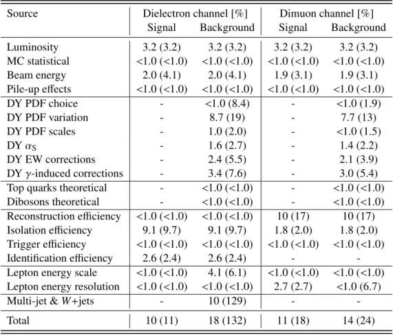
Table 2: Summary of the pre-marginalised relative systematic uncertainties in the expected number of events at dilepton masses of 2 TeV and 4 TeV. The values reported in parenthesis correspond to the 4 TeV mass. The values quoted for the background represent the relative change in the total expected number of events in the corresponding m``histogram bin containing the reconstructed m``mass of 2 TeV (4 TeV). For the signal uncertainties the values
were computed using a Z0
χsignal model with a pole mass of 2 TeV (4 TeV) by comparing yields in the core of the
mass peak (within the full width at half maximum) between the distribution varied due to a given uncertainty and the nominal distribution. “-” represents cases where the uncertainty is not applicable.
Source Dielectron channel [%] Dimuon channel [%]
Signal Background Signal Background
Luminosity 3.2 (3.2) 3.2 (3.2) 3.2 (3.2) 3.2 (3.2) MC statistical <1.0 (<1.0) <1.0 (<1.0) <1.0 (<1.0) <1.0 (<1.0) Beam energy 2.0 (4.1) 2.0 (4.1) 1.9 (3.1) 1.9 (3.1) Pile-up effects <1.0 (<1.0) <1.0 (<1.0) <1.0 (<1.0) <1.0 (<1.0) DY PDF choice - <1.0 (8.4) - <1.0 (1.9) DY PDF variation - 8.7 (19) - 7.7 (13) DY PDF scales - 1.0 (2.0) - <1.0 (1.5) DY αS - 1.6 (2.7) - 1.4 (2.2) DY EW corrections - 2.4 (5.5) - 2.1 (3.9) DY γ-induced corrections - 3.4 (7.6) - 3.0 (5.4)
Top quarks theoretical - <1.0 (<1.0) - <1.0 (<1.0)
Dibosons theoretical - <1.0 (<1.0) - <1.0 (<1.0)
Reconstruction efficiency <1.0 (<1.0) <1.0 (<1.0) 10 (17) 10 (17)
Isolation efficiency 9.1 (9.7) 9.1 (9.7) 1.8 (2.0) 1.8 (2.0)
Trigger efficiency <1.0 (<1.0) <1.0 (<1.0) <1.0 (<1.0) <1.0 (<1.0)
Identification efficiency 2.6 (2.4) 2.6 (2.4) -
-Lepton energy scale <1.0 (<1.0) 4.1 (6.1) <1.0 (<1.0) <1.0 (<1.0) Lepton energy resolution <1.0 (<1.0) <1.0 (<1.0) 2.7 (2.7) <1.0 (6.7)
Multi-jet & W+jets - 10 (129) -
calibration of the luminosity scale using x–y beam-separation scans performed in August 2015 and May 2016. Systematic uncertainties used in the statistical analysis of the results are summarised in Table2at dilepton mass values of 2 TeV and 4 TeV. The systematic uncertainties are constrained in the likelihood during the statistical interpretation through a marginalisation procedure, as described in Section9.
8 Event yields
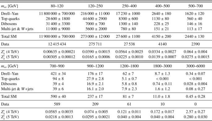
Expected and observed event yields, in bins of invariant mass, are shown in Table3for the dielectron channel, and in Table4for the dimuon channel. Expected event yields are split into the different back-ground sources and the yields for two signal scenarios are also provided. In general, the observed data are in good agreement with the SM prediction, taking into account the uncertainties as described in Sec-tion7.
Table 3: Expected and observed event yields in the dielectron channel in different dilepton mass intervals. The quoted errors correspond to the combined statistical, theoretical, and experimental systematic uncertainties. Expec-ted event yields are reporExpec-ted for the Z0
χmodel, for two values of the pole mass. All numbers shown are obtained
before the marginalisation procedure.
mee[GeV] 80–120 120–250 250–400 400–500 500–700
Drell–Yan 11 800 000 ± 700 000 216 000 ± 11 000 17 230 ± 1000 2640 ± 180 1620 ± 120 Top quarks 28 600 ± 1800 44 600 ± 2900 8300 ± 600 1130 ± 80 560 ± 40 Dibosons 31 400 ± 3300 7000 ± 700 1300 ± 140 228 ± 25 146 ± 16 Multi-jet & W+jets 11 000 ± 9000 5600 ± 2000 780 ± 80 151 ± 21 113 ± 17 Total SM 11 900 000 ± 700 000 273 000 ± 12 000 27 600 ± 1100 4150 ± 200 2440 ± 130 Data 12 415 434 275 711 27 538 4140 2390 Z0 χ(4 TeV) 0.00635 ± 0.00021 0.0390 ± 0.0015 0.0564 ± 0.0025 0.0334 ± 0.0027 0.064 ± 0.004 Z0 χ(5 TeV) 0.00305 ± 0.00012 0.0165 ± 0.0006 0.0225 ± 0.0010 0.0139 ± 0.0007 0.0275 ± 0.0015 mee[GeV] 700–900 900–1200 1200–1800 1800–3000 3000–6000 Drell–Yan 421 ± 34 176 ± 17 62 ± 7 8.7 ± 1.3 0.34 ± 0.07 Top quarks 94 ± 8 27.9 ± 2.8 5.1 ± 0.7 < 0.001 < 0.001 Dibosons 39 ± 4 16.9 ± 2.1 5.8 ± 0.8 0.74 ± 0.11 0.028 ± 0.004 Multi-jet & W+jets 39 ± 6 16.1 ± 2.0 7.9 ± 2.3 1.6 ± 1.2 0.08 ± 0.27 Total SM 590 ± 40 237 ± 17 81 ± 7 11.0 ± 1.8 0.45 ± 0.28 Data 589 209 61 10 0 Z0 χ(4 TeV) 0.0585 ± 0.0035 0.074 ± 0.005 0.121 ± 0.011 0.172 ± 0.017 2.57 ± 0.27 Z0 χ(5 TeV) 0.0218 ± 0.0013 0.0295 ± 0.0021 0.040 ± 0.004 0.040 ± 0.004 0.280 ± 0.030
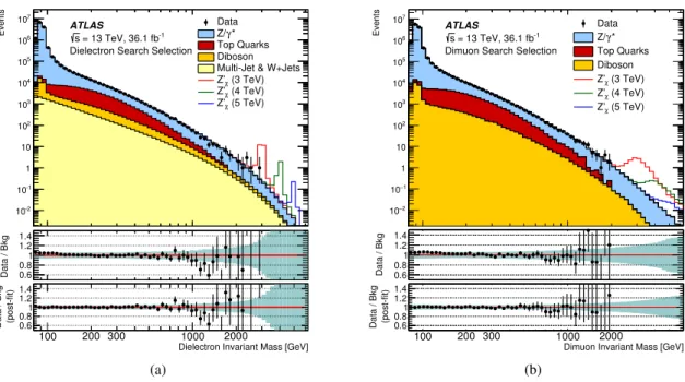
Distributions of m`` in the dielectron and dimuon channels are shown in Figure 1. No clear excess is observed, but significances are quantified and discussed in Section9. The highest dilepton invariant mass event is 2.90 TeV in the dielectron channel, and 1.99 TeV in the dimuon channel. Both of these events are well-measured with little other detector activity.
Table 4: Expected and observed event yields in the dimuon channel in different dilepton mass intervals. The quoted errors correspond to the combined statistical, theoretical, and experimental systematic uncertainties. Expected event yields are reported for the Z0
χmodel, for two values of the pole mass. All numbers shown are obtained before the
marginalisation procedure. mµµ[GeV] 80–120 120–250 250–400 400–500 500–700 Drell–Yan 10 700 000 ± 600 000 177 900 ± 10 000 12 200 ± 700 1770 ± 120 1060 ± 80 Top quarks 24 700 ± 1700 34 200 ± 2400 6100 ± 500 830 ± 70 401 ± 33 Dibosons 26 000 ± 2800 5400 ± 600 910 ± 100 155 ± 17 93 ± 11 Total SM 10 800 000 ± 600 000 218 000 ± 10 000 19 200 ± 900 2760 ± 140 1550 ± 90 Data 11 321 561 224 703 19 239 2766 1532 Z0 χ(4 TeV) 0.00873 ± 0.00032 0.0334 ± 0.0015 0.0441 ± 0.0021 0.0246 ± 0.0014 0.052 ± 0.004 Z0 χ(5 TeV) 0.00347 ± 0.00014 0.0137 ± 0.0006 0.0151 ± 0.0007 0.0105 ± 0.0006 0.0176 ± 0.0012 mµµ[GeV] 700–900 900–1200 1200–1800 1800–3000 3000–6000 Drell–Yan 263 ± 23 110 ± 11 37 ± 4 5.4 ± 0.8 0.30 ± 0.07 Top quarks 68 ± 6 24.5 ± 3.0 5.3 ± 0.9 0.11 ± 0.08 < 0.001 Dibosons 24.3 ± 2.9 9.8 ± 1.2 3.2 ± 0.4 0.45 ± 0.07 0.0184 ± 0.0035 Total SM 355 ± 24 144 ± 11 45 ± 4 6.0 ± 0.8 0.32 ± 0.07 Data 322 141 48 4 0 Z0 χ(4 TeV) 0.0362 ± 0.0026 0.048 ± 0.004 0.067 ± 0.006 0.186 ± 0.022 1.24 ± 0.19 Z0 χ(5 TeV) 0.0153 ± 0.0011 0.0185 ± 0.0015 0.0233 ± 0.0021 0.0258 ± 0.0029 0.118 ± 0.020
9 Statistical analysis
The m`` distributions are scrutinised for a resonant or non-resonant new physics excess using two meth-ods and are used to set limits on resonant and non-resonant new physics models, as well as on generic resonances. Tabulated values of all the observed results, along with their uncertainties, are also provided in the Durham HEP database [53]. The signal search and limit setting rely on a likelihood function, de-pendent on the parameter of interest, such as the signal cross-section, signal strength, coupling constant or the contact interaction scale. The likelihood function also depends on nuisance parameters which de-scribe the systematic uncertainties. In this analysis the data are assumed to be Poisson-distributed in each bin of the m`` distribution and the likelihood is constructed as a product of individual bin likelihoods. In case of the individual channel results, the product is taken over the bins of the m`` histogram in the given channel, while for combined results the product is taken over bins of histograms in dielectron and
dimuon channels. The logarithmic m`` histogram binning shown in Figure1 uses 66 mass bins and is
chosen for setting limits on resonant signals. This binning is optimal for resonances with a width of 3%, therefore the chosen bin width for the m`` histogram in the search phase corresponds to the resolution in the dielectron (dimuon) channel, which varies from 10 (60) GeV at m``= 1 TeV to 15 (200) GeV at m`` = 2 TeV, and 20 (420) GeV at m`` = 3 TeV. For setting limits on the contact interaction scale, the m`` distribution has eight bins above 400 GeV with bin widths varying from 100 to 1500 GeV. The m``region from 80 to 120 GeV is included in the likelihood as a single bin in the limit setting on resonant signals to help constrain mass-independent components of systematic uncertainties, but that region is not searched for a new-physics signal.
90
100200
1000
2000
Events -2 10 -1 10 1 10 2 10 3 10 4 10 5 10 6 10 7 10 Data * γ Z/ Top Quarks Diboson Multi-Jet & W+Jets(3 TeV) χ Z’ (4 TeV) χ Z’ (5 TeV) χ Z’ ATLAS -1 = 13 TeV, 36.1 fb s
Dielectron Search Selection
Data / Bkg 0.60.8 1 1.2 1.4
Dielectron Invariant Mass [GeV]
100 200 300 1000 2000 (post-fit) Data / Bkg 0.6 0.81 1.2 1.4 (a) Events 2 − 10 1 − 10 1 10 2 10 3 10 4 10 5 10 6 10 7 10 Data * γ Z/ Top Quarks Diboson (3 TeV) χ Z’ (4 TeV) χ Z’ (5 TeV) χ Z’ ATLAS -1 = 13 TeV, 36.1 fb s
Dimuon Search Selection
Data / Bkg 0.6 0.8 1 1.2 1.4
Dimuon Invariant Mass [GeV]
100 200 300 1000 2000 (post-fit) Data / Bkg 0.6 0.81 1.2 1.4 (b)
Figure 1: Distributions of(a)dielectron and(b)dimuon reconstructed invariant mass (m``) after selection, for data
and the SM background estimates as well as their ratio before and after marginalisation. Selected Z0
χsignals with a
pole mass of 3, 4 and 5 TeV are overlaid. The bin width of the distributions is constant in log(m``) and the shaded band in the lower panels illustrates the total systematic uncertainty, as explained in Section7. The data points are shown together with their statistical uncertainty. Exact bin edges and contents are provided in Table8and Table9 in the appendix.
the dilepton final state (σB) to its theoretically predicted value. Upper limits on σB for specific Z0boson models and generic Z0bosons, γ0of the Minimal Z0boson, and lower limit on the CI scaleΛ are set in a Bayesian approach. The calculations are performed with the Bayesian Analysis Toolkit (BAT) [54], which uses a Markov Chain MC (MCMC) technique to compute the marginal posterior probability density of the parameter of interest (so-called “marginalisation”). Limit values obtained using the experimental data are quoted as observed limits, while median values of the limits obtained from a large number of simulated experiments, where only SM background is present, are quoted as the expected limits. The upper limits on σB are interpreted as lower limits on the Z0pole mass using the relationship between the pole mass and the theoretical Z0 cross-section. In the context of the Minimal Z0 model or CI scenarios, limits are set on the parameter of interest. In the case of the Minimal Z0model the parameter of interest is γ04. For a CI the parameter of interest is set either to 1/Λ2 or to 1/Λ4 as this corresponds to the scaling of the CI–SM interference contribution or the pure CI contribution respectively. In both the Minimal Z0and the CI cases, the nominal Poisson expectation in each m``bin is expressed as a function of the parameter of interest. As in the context of the Z0limit setting, the Poisson mean is modified by shifts due to systematic uncertainties, but in both the Minimal Z0 and the CI cases, these shifts are non-linear functions of the parameter of interest. A prior uniform in the parameter of interest is used for all limits.
Two complementary approaches are used in the search for a new-physics signal. The first approach, which does not rely on a specific signal model and therefore is sensitive to a wide range of new physics, uses the BumpHunter (BH) [55] utility. In this approach, all consecutive intervals in the m`` histogram ranging from two bins to half of the bins in the histogram are searched for an excess. In each such interval a Poisson probability (p-value) is computed for an event count greater or equal to the number observed
found in data, given the SM prediction. The modes of marginalised posteriors of the nuisance parameters from the MCMC method are used to construct the SM prediction. The negative logarithm of the smallest p-value is the BH statistic. The BH statistic is then interpreted as a global p-value utilising simulated experiments where, in each simulated experiment, simulated data is generated from SM background model. The dielectron and dimuon channels are tested separately.
A search for Zχ0 signals as well as generic Z0signals with widths from 1% to 12% is performed utilising the log-likelihood ratio (LLR) test described in Ref. [56]. This second approach is specifically sensitive to narrow Z0-like signals, and is thus complementary to the more general BH approach. To perform the LLR search, the Histfactory [57] package is used together with the RooStats [58] and RooFit [59] packages. The p-value for finding a Z0χsignal excess (at a given pole mass), or a variable width generic Z0excess (at a given central mass and with a given width), more significant than that observed in the data, is computed analytically, using a test statistic q0. The test statistic q0is based on the logarithm of the profile likelihood ratio λ(µ). The test statistic is modified for signal masses below 1.5 TeV to also quantify the significance of potential deficits in the data. As in the BH search the SM background model is constructed using the modes of marginalised posteriors of the nuisance parameters from the MCMC method, and these nuisance parameters are not included in the likelihood at this stage. Therefore, in the search-phase the background estimate and signal shapes are fixed to their post-marginalisation estimates, and systematic uncertainties are not included in the computation of the p-value. Starting with MZ0 = 150 GeV, multiple
mass hypotheses are tested in pole-mass steps corresponding to the histogram bin width to compute the local p-values — i.e. p-values corresponding to specific signal mass hypotheses. Simulated experiments (for MZ0 > 1.5 TeV) and asymptotic relations (for MZ0 < 1.5 TeV) in Ref. [56] are used to estimate the
global p-value, which is the probability to find anywhere in the m`` distribution a Z0-like excess more significant than that observed in the data.
10 Results
The data, scrutinised using the statistical tests described in the previous section, show no significant excesses. The LLR tests for a Zχ0 resonance find global p-values of 58%, 91% and 83% in the dielectron,
dimuon, and combined channels, respectively. The local and global p-values as a function of the Z0
pole mass are shown in Figure2. The un-capped p-value, is used below a pole mass of 1.5 TeV, which
quantifies both excesses and deficits, while above 1.5 TeV the signal strength parameter is constrained to be positive, yielding a capped p-value. This constraint is used in the high mass region where the expected background is very low, to avoid ill-defined configurations of the probability density function in the likelihood fit, with negative probabilities.
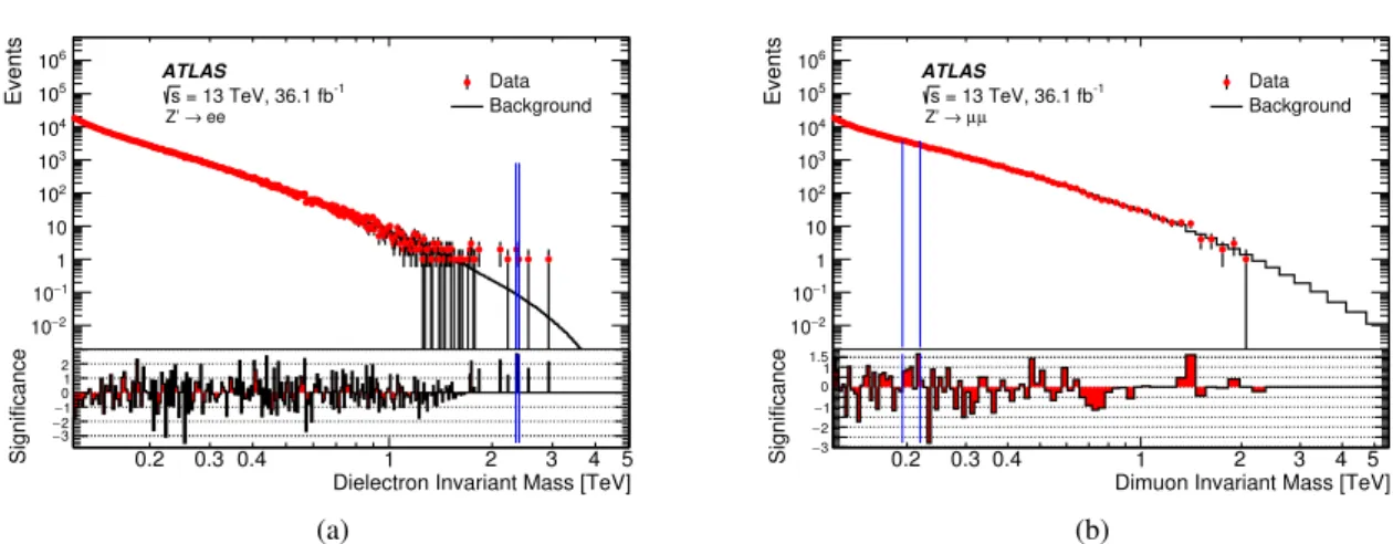
The largest deviation from the background-only hypothesis using the LLR tests for a Zχ0 is observed at 2.37 TeV in the dielectron mass spectrum with a local significance of 2.5 σ, but globally the excess is not significant. The BumpHunter [55] test, which scans the mass spectrum with varying intervals to find the most significant excess in data, finds p-values of 71% and 94% in the dielectron and dimuon channels, respectively. Figure3shows the dilepton mass distribution in the dielectron and dimuon channels with the observed data overlaid on the combined background prediction, and also the local significance. The interval with the largest upward deviation is indicated by a pair of blue lines.
[TeV] Z’ M 0.2 0.3 0.4 1 2 3 4 0 Local p 3 − 10 2 − 10 1 − 10 1 10 2 10 σ 0 Local significance σ 1 σ 2 σ 3 σ 0
Global significance for largest excess σ 1 ATLAS -1 = 13 TeV, 36.1 fb s ll → χ , Z’ 0 Observed p
Figure 2: The local p-value derived assuming Z0
χsignal shapes with pole masses between 0.15 and 4.0 TeV for
the combined dilepton channel. Accompanying local and global significance levels are shown as dashed lines. The uncapped p0value is used for pole masses below 1.5 TeV, while the capped p0value is used for higher pole masses.
0.2 0.3 0.4 1 2 3 4 5 Events 3 − 10 2 − 10 1 − 10 1 10 2 10 3 10 4 10 5 10 6 10 Data Background -1 = 13 TeV, 36.1 fb s ee → Z’ ATLAS
Dielectron Invariant Mass [TeV] 0.2 0.3 0.4 1 2 3 4 5 Significance 3 − 2 − 1 − 01 2 (a) 0.2 0.3 0.4 1 2 3 4 5 Events 3 − 10 2 − 10 1 − 10 1 10 2 10 3 10 4 10 5 10 6 10 Data Background -1 = 13 TeV, 36.1 fb s µ µ → Z’ ATLAS
Dimuon Invariant Mass [TeV] 0.2 0.3 0.4 1 2 3 4 5 Significance −3 2 − 1 − 0 1 1.5 (b)
Figure 3: Dilepton mass distribution in the(a) dielectron and (b) dimuon channel, showing the observed data together with their statistical uncertainty, combined background prediction, and corresponding bin-by-bin signific-ance. The most significant interval is indicated by the vertical blue lines. Exact bin edges and contents are provided in Table10and Table11in the appendix.
10.1 Z0cross-section and mass limits
Upper limits on the cross-section times branching ratio (σB) for Z0bosons are presented in Figure4. The observed and expected lower limits on the pole mass for various Z0scenarios, as described in Section2.1, are summarised in Table5. The Z0χsignal is used to extract the limits, which is over-conservative for the other E6models presented, but slightly under-conservative for the ZSSM0 , although only by 100 GeV in the mass limit at most. The upper limits on σB for Z0bosons start to weaken above a pole mass of ∼ 3.5 TeV. The effect is more pronounced in the dimuon channel due to worse mass resolution than in the dielectron channel. The weakening is mainly due to the combined effect of a rapidly falling signal cross-section as the kinematic limit is approached, with an increasing proportion of the signal being produced off-shell in the low-mass tail, and the natural width of the resonance. The selection efficiency also starts to slowly decrease at very high pole masses, but this is a subdominant effect.
[TeV] Z’ M 0.5 1 1.5 2 2.5 3 3.5 4 4.5 5 B [pb] σ -5 10 -4 10 -3 10 -2 10 -1 10 1 Expected limit σ 1 ± Expected σ 2 ± Expected Observed limit SSM Z’ χ Z’ ψ Z’ ATLAS ll → Z’ -1 = 13 TeV, 36.1 fb s
Figure 4: Upper 95% CL limits on the Z0production cross-section times branching ratio to two leptons of a single flavour as a function of Z0pole mass (MZ0). Results are shown for the combined dilepton channel. The signal
theoretical σB are calculated with Pythia 8 using the NNPDF23LO PDF set [36], and corrected to next-to-next-to-leading order in QCD using VRAP [28] and the CT14NNLO PDF set [29]. The signals theoretical uncertainties are shown as a band on the Z0
SSMtheory line for illustration purposes, but are not included in the σB limit calculation.
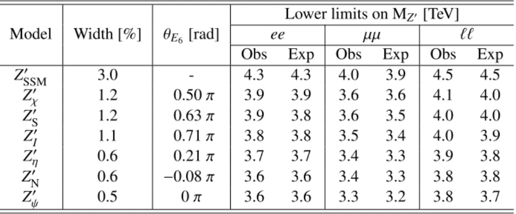
Table 5: Observed and expected 95% CL lower mass limits for various Z0gauge boson models. The widths are quoted as a percentage of the resonance mass.
Model Width [%] θE6 [rad]
Lower limits on MZ0[TeV]
ee µµ ``
Obs Exp Obs Exp Obs Exp
ZSSM0 3.0 - 4.3 4.3 4.0 3.9 4.5 4.5 Zχ0 1.2 0.50 π 3.9 3.9 3.6 3.6 4.1 4.0 ZS0 1.2 0.63 π 3.9 3.8 3.6 3.5 4.0 4.0 Z0I 1.1 0.71 π 3.8 3.8 3.5 3.4 4.0 3.9 Zη0 0.6 0.21 π 3.7 3.7 3.4 3.3 3.9 3.8 ZN0 0.6 −0.08 π 3.6 3.6 3.4 3.3 3.8 3.8 Zψ0 0.5 0 π 3.6 3.6 3.3 3.2 3.8 3.7
10.2 Limits on Minimal Z0models
Limits are set on the relative coupling strength of the Z0 boson relative to that of the SM Z boson (γ0) as a function of the ZMin0 boson mass, and as a function of the mixing angle θMin, as shown in Figure5, and
described in Section2.2. The two θMin values yielding the minimum and maximum cross-sections are
used to define a band of limits in the (γ0, MZMin) plane. It is possible to put lower mass limits on specific
models which are covered by the (γ0, θMin) parameterisation as in Table6. The structure observed in the limits as a function of θMin, such as the maximum around θMin= 2.2, is due to the changing shape of the resonance at a given pole mass, from narrow to wide.
[TeV] Min Z’ M 0.5 1 1.5 2 2.5 3 3.5 4 4.5 5 ’ γ 2 − 10 1 − 10 1 10 Exp. Obs. ] π [0, ∈ Min θ Limit range for
) χ (Z’ Min θ ) 3R (Z’ Min θ ) B-L (Z’ Min θ ATLAS -1 = 13 TeV, 36.1 fb s ll → Min Z’ (a) Min θ 0 0.5 1 1.5 2 2.5 3 ’ γ 2 − 10 1 − 10 1 10 Exp. Obs. = 5.0 TeV Min Z’ M = 4.5 TeV Min Z’ M = 4.0 TeV Min Z’ M = 3.5 TeV Min Z’ M = 3.0 TeV Min Z’ M = 2.5 TeV Min Z’ M = 2.0 TeV Min Z’ M = 1.5 TeV Min Z’ M = 1.0 TeV Min Z’ M = 0.5 TeV Min Z’ M ATLAS -1 = 13 TeV, 36.1 fb s ll → Min Z’ (b)
Figure 5:(a)Expected (dotted and dashed lines) and observed (filled area and lines) limits are set at 95% CL on the relative coupling strength γ0for the dilepton channel as a function of the Z0Minmass in the Minimal Z0model. Limit curves are shown for three representative values of the mixing angle, θMin, between the generators of the
(B − L) and the weak hypercharge Y gauge groups. These are: tan θMin = 0, tan θMin = −2 and tan θMin = −0.8,
which correspond respectively to the Z0 B-L, Z
0 3Rand Z
0
χmodels at specific values of γ0. The region above each line
is excluded. The grey band envelops all observed limit curves, which depend on the choice of θMin ∈ [0, π]. The
corresponding expected limit curves are within the area delimited by the two dotted lines. (b) Expected (empty markers and dashed lines) and observed (filled markers and lines) limits at 95% CL on γ0for the dilepton channel
as a function of θMin. The limits are set for several representative values of the mass of the Z0boson, MZ0 Min. The
region above each line is excluded.
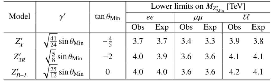
Table 6: Observed and expected 95% CL lower mass limits for various ZMin0 models.
Model γ0 tan θMin
Lower limits on MZ0
Min[TeV]
ee µµ ``
Obs Exp Obs Exp Obs Exp
Zχ0 q 41 24sin θMin − 4 5 3.7 3.7 3.4 3.3 3.9 3.8 Z3R0 q 5 8sin θMin −2 4.0 3.9 3.6 3.6 4.1 4.1 Z0B−L q 25 12sin θMin 0 4.0 4.0 3.6 3.6 4.2 4.1
10.3 Generic Z0 limits
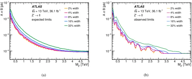
In order to derive more general limits, an approach which compares the data to signals that are more model-independent was developed. This was achieved by applying fiducial cuts to the signal (lepton pT > 30 GeV, and lepton |η| < 2.5) and a mass window of two times the true signal width (width of the Breit–Wigner) around the pole mass of the signal. This is expected to give limits that are more model independent since any effect on the sensitivity due to the tails of the resonance, foremost the parton luminosity tail and interference effects, are removed. The resulting limits can be seen in Figure6. For other models to be interpreted with these cross-section limits, the acceptance for a given model in the same fiducial region should be calculated, multiplied by the total cross-section, and the resulting acceptance-corrected cross-section theory curve overlaid, to extract the mass limit for that model. The dilepton invariant mass shape, and angular distributions for the chosen model, should be sufficiently close to a generic Z0resonance, such as those presented in this article, so as not to induce additional efficiency differences. [TeV] Z’ M 0.5 1 1.5 2 2.5 3 3.5 4 4.5 5 B [pb] σ A 4 − 10 3 − 10 2 − 10 1 − 10 2% width 4% width 8% width 16% width 32% width ATLAS ll → Z’ -1 = 13 TeV, 36.1 fb s expected limits (a) [TeV] Z’ M 0.5 1 1.5 2 2.5 3 3.5 4 4.5 5 B [pb] σ A 4 − 10 3 − 10 2 − 10 1 − 10 2% width 4% width 8% width 16% width 32% width ATLAS ll → Z’ -1 = 13 TeV, 36.1 fb s observed limits (b)
Figure 6: Upper 95% CL limits on the acceptance times Z0production cross-section times branching ratio to two
leptons of a single flavour as a function of Z0pole mass (M
Z0).(a)Expected and(b)observed limits in the combined
dilepton channel for different widths with an applied mass window of two times the true width of the signal around the pole mass.
10.4 Limits on the energy scale of Contact Interactions
Lower limits are set at 95% CL on the energy scaleΛ, for the LL, LR, RL, and RR Contact Interaction
model, as described in Section2.3. Both the constructive and destructive interference scenarios are ex-plored, as well as priors of 1/Λ2 and 1/Λ4. Limits are presented for the combined dilepton channel in Figure7using a 1/Λ2prior. All of the CI exclusion limits are summarised in Table7.
Chiral Structure
LL Const LL Dest LR Const LR Dest RL Const RL Dest RR Const RR Dest
[TeV] Λ 20 25 30 35 40 45 50 55 Observed Expected σ 1 ± Expected σ 2 ± Expected ATLAS -1 = 13 TeV, 36.1 fb s 2 Λ Prior: 1/ ll → CI
Figure 7: Lower limits on the energy scaleΛ at 95% CL, for the Contact Interaction model with constructive (const) and destructive (dest) interference, and all considered chiral structures with left-handed (L) and right-handed (R) couplings. Results are shown for the combined dilepton channel.
Table 7: Observed and expected 95% CL lower limits onΛ for the LL, LR, RL, and RR chiral coupling scenarios, for both the constructive (const) and destructive (dest) interference cases using a uniform positive prior in 1/Λ2or
1/Λ4. The dielectron, dimuon, and combined dilepton channel limits are shown, rounded to two significant figures.
Channel Prior
Lower limits onΛ [TeV]
Left–Left Left–Right Right–Left Right–Right
Const Dest Const Dest Const Dest Const Dest
Obs: ee 1/Λ2 37 24 33 26 33 26 33 26 Exp: ee 28 22 26 23 26 23 25 23 Obs: ee 1/Λ4 32 22 29 24 29 24 29 24 Exp: ee 26 20 24 21 24 21 24 21 Obs: µµ 1/Λ2 30 20 28 22 28 22 28 20 Exp: µµ 26 20 24 21 24 21 24 20 Obs: µµ 1/Λ4 27 19 25 21 25 21 25 19 Exp: µµ 24 18 23 20 22 20 22 18 Obs: `` 1/Λ2 40 25 36 28 35 28 35 28 Exp: `` 31 23 28 24 28 24 28 24 Obs: `` 1/Λ4 35 24 32 25 32 25 31 25 Exp: `` 28 21 26 22 26 23 26 22
11 Conclusion
The ATLAS detector at the LHC has been used to search for both resonant and non-resonant new phe-nomena in the dilepton invariant mass spectrum above the Z boson’s pole. The search is conducted with 36.1 fb−1of pp collision data at √s= 13 TeV, recorded during 2015 and 2016. The highest invariant mass event is found at 2.90 TeV in the dielectron channel, and 1.99 TeV in the dimuon channel. The observed dilepton invariant mass spectrum is consistent with the Standard Model prediction, within systematic and statistical uncertainties. Among a choice of different models, the data are interpreted in terms of resonant spin-1 Z0gauge boson production and non-resonant qq`` contact interactions. For the resonant interpret-ation, upper limits are set on the cross-section times branching ratio for a spin-1 Z0 gauge boson. The resulting 95% CL lower mass limits are 4.5 TeV for the ZSSM0 , 4.1 TeV for the Zχ0, and 3.8 TeV for the Zψ0. Other E6Z0 models are also constrained in the range between those quoted for the Zχ0 and Zψ0. This result is more stringent than the previous ATLAS result at √s= 13 TeV obtained with 2015 data, by up to 700 GeV. Lower mass limits are also set on the Minimal Z0 model, up to 4.1 TeV for the Z3R0 , and 4.2 TeV for the ZB-L0 . Generic Z0cross-section limits are also provided for a range of true signal widths. The lower limits on the energy scaleΛ for various qq`` contact interaction models range between 24 TeV and 40 TeV, which are more stringent than the previous ATLAS result obtained at √s= 13 TeV, by up to 4 TeV.
Appendix
This appendix provides the exact bin edges and contents of the dilepton invariant mass plots presented in Figures1(a),1(b),3(a), and3(b). These correspond to Tables8,9,10, and11, respectively. Even more detailed information can be found in the Durham HEP database [53].
Table 8: Expected and observed event yields in the dielectron channel, directly corresponding to the non-linear binning presented in Figure1(a). The expected yield is given up to at most 4 digit precision.
Lower edge [GeV] Upper edge [GeV] Data [N] Total Background [N]
80 85.549 1176847 1112000 85.549 91.482 6608874 6322000 91.482 97.828 3928394 3756000 97.828 104.61 432217 414400 104.61 111.87 162962 156100 111.87 119.63 93773 90620 119.63 127.93 63446 62270 127.93 136.8 47190 46740 136.8 146.29 36539 36090 146.29 156.43 29267 28990 156.43 167.28 23874 23740 167.28 178.89 19689 19550 178.89 191.29 16548 16400 191.29 204.56 13671 13590 204.56 218.75 11337 11460 218.75 233.92 9358 9499 233.92 250.15 7877 7868 250.15 267.5 6434 6570 267.5 286.05 5500 5427 286.05 305.89 4445 4477 305.89 327.11 3648 3667 327.11 349.79 2981 2995 349.79 374.06 2431 2403 374.06 400 1964 1957 400 427.74 1606 1565 427.74 457.41 1231 1265 457.41 489.14 1013 1008 489.14 523.06 776 805.6 523.06 559.34 622 628.7 559.34 598.14 464 492.3 598.14 639.63 403 392.6 639.63 683.99 300 304.4 683.99 731.43 219 234.3 731.43 782.16 202 183.2 782.16 836.41 133 140.2 836.41 894.43 107 107.1 894.43 956.46 82 85.13 956.46 1022.8 57 63.86 1022.8 1093.7 43 47.9 1093.7 1169.6 27 38.09 1169.6 1250.7 24 28.7 1250.7 1337.5 12 20.28 1337.5 1430.2 13 14.96 1430.2 1529.4 11 11.16
1529.4 1635.5 3 8.262 1635.5 1749 7 6.003 1749 1870.3 4 4.085 1870.3 2000 0 2.875 2000 2138.7 2 2.05 2138.7 2287.1 1 1.431 2287.1 2445.7 3 0.977 2445.7 2615.3 1 0.655 2615.3 2796.7 0 0.443 2796.7 2990.7 1 0.284 2990.7 3198.1 0 0.183 3198.1 3420 0 0.114 3420 3657.2 0 0.068 3657.2 3910.8 0 0.041 3910.8 4182.1 0 0.023 4182.1 4472.1 0 0.013 4472.1 4782.3 0 0.007 4782.3 5114 0 0.004 5114 5468.7 0 0.002 5468.7 5848 0 0.001 5848 6253.7 0 0
Table 9: Expected and observed event yields in the dimuon channel, directly corresponding to the non-linear binning presented in Figure1(b). The expected yield is given up to at most 4 digit precision.
Lower edge [GeV] Upper edge [GeV] Data [N] Total Background [N]
80 85.549 826504 786600 85.549 91.482 5730639 5465000 91.482 97.828 4062661 3848000 97.828 104.61 430822 405500 104.61 111.87 149927 141800 111.87 119.63 82971 79230 119.63 127.93 54641 52110 127.93 136.8 39501 37890 136.8 146.29 29742 28940 146.29 156.43 23871 23220 156.43 167.28 18942 18490 167.28 178.89 15482 15140 178.89 191.29 12495 12250 191.29 204.56 10462 10230 204.56 218.75 8583 8261 218.75 233.92 6868 6885 233.92 250.15 5649 5517 250.15 267.5 4723 4607 267.5 286.05 3762 3753 286.05 305.89 3064 3106 305.89 327.11 2471 2566 327.11 349.79 2031 1992 349.79 374.06 1595 1628 374.06 400 1333 1321 400 427.74 1018 1022 427.74 457.41 819 828.1 457.41 489.14 675 651.9 489.14 523.06 508 513.6 523.06 559.34 397 410.7
559.34 598.14 306 306 598.14 639.63 252 245.7 639.63 683.99 188 191.2 683.99 731.43 129 142.2 731.43 782.16 97 108.5 782.16 836.41 78 82.36 836.41 894.43 57 63.72 894.43 956.46 51 51.88 956.46 1022.8 39 39.04 1022.8 1093.7 29 29.74 1093.7 1169.6 18 21.83 1169.6 1250.7 18 16.12 1250.7 1337.5 14 12.7 1337.5 1430.2 12 8.053 1430.2 1529.4 5 5.803 1529.4 1635.5 4 4.667 1635.5 1749 1 3.241 1749 1870.3 4 2.135 1870.3 2000 2 1.663 2000 2138.7 0 1.102 2138.7 2287.1 0 0.763 2287.1 2445.7 0 0.538 2445.7 2615.3 0 0.375 2615.3 2796.7 0 0.250 2796.7 2990.7 0 0.165 2990.7 3198.1 0 0.112 3198.1 3420 0 0.078 3420 3657.2 0 0.049 3657.2 3910.8 0 0.031 3910.8 4182.1 0 0.022 4182.1 4472.1 0 0.013 4472.1 4782.3 0 0.010 4782.3 5114 0 0.006 5114 5468.7 0 0.005 5468.7 5848 0 0.002 5848 6253.7 0 0.002
Table 10: Expected and observed event yields in the dielectron channel, directly corresponding to the non-linear binning presented in Figure3(a). The expected yield is given up to at most 4 digit precision.
Lower edge [TeV] Upper edge [TeV] Data [N] Total Background [N] 0.11962 0.12171 18432 18660 0.12171 0.12381 16720 16840 0.12381 0.12592 15291 15340 0.12592 0.12806 13924 14020 0.12806 0.13022 12931 12960 0.13022 0.13239 11976 11970 0.13239 0.13459 11154 11120 0.13459 0.1368 10273 10350 0.1368 0.13903 9637 9677 0.13903 0.14128 9017 9029 0.14128 0.14355 8392 8460 0.14355 0.14584 8043 7949 0.14584 0.14815 7387 7507 0.14815 0.15048 7122 7073
0.15048 0.15283 6695 6680 0.15283 0.1552 6382 6278 0.1552 0.15758 5933 6018 0.15758 0.15999 5737 5697 0.15999 0.16242 5352 5380 0.16242 0.16487 5097 5158 0.16487 0.16733 4972 4893 0.16733 0.16982 4726 4622 0.16982 0.17233 4455 4437 0.17233 0.17486 4165 4198 0.17486 0.17741 3979 4058 0.17741 0.17998 3920 3868 0.17998 0.18257 3629 3687 0.18257 0.18518 3671 3531 0.18518 0.18782 3392 3349 0.18782 0.19047 3154 3207 0.19047 0.19315 3182 3081 0.19315 0.19584 2964 2957 0.19584 0.19856 2826 2825 0.19856 0.2013 2687 2712 0.2013 0.20406 2637 2593 0.20406 0.20685 2380 2510 0.20685 0.20965 2436 2396 0.20965 0.21248 2223 2295 0.21248 0.21533 2166 2202 0.21533 0.2182 2152 2089 0.2182 0.2211 2030 2003 0.2211 0.22402 1803 1938 0.22402 0.22696 1869 1831 0.22696 0.22992 1736 1774 0.22992 0.23291 1788 1726 0.23291 0.23591 1605 1646 0.23591 0.23895 1651 1576 0.23895 0.242 1530 1515 0.242 0.24508 1386 1453 0.24508 0.24818 1398 1398 0.24818 0.25131 1354 1328 0.25131 0.25446 1171 1297 0.25446 0.25763 1293 1246 0.25763 0.26083 1139 1191 0.26083 0.26405 1187 1155 0.26405 0.2673 1075 1117 0.2673 0.27057 1051 1073 0.27057 0.27387 1045 1022 0.27387 0.27719 1011 988.8 0.27719 0.28053 953 943.4 0.28053 0.2839 966 908.3 0.2839 0.2873 834 878.5 0.2873 0.29072 820 840.8 0.29072 0.29416 813 809.1 0.29416 0.29764 799 782.9 0.29764 0.30113 723 742.1 0.30113 0.30466 746 722.8 0.30466 0.30821 692 696.2 0.30821 0.31178 655 668.4 0.31178 0.31539 639 656.2 0.31539 0.31901 607 615.3
0.31901 0.32267 594 597.5 0.32267 0.32635 586 568.5 0.32635 0.33006 560 550.5 0.33006 0.3338 524 520.3 0.3338 0.33756 475 512.2 0.33756 0.34135 500 499 0.34135 0.34517 490 466.4 0.34517 0.34902 465 443.6 0.34902 0.35289 443 436.7 0.35289 0.3568 417 420.2 0.3568 0.36073 413 393.5 0.36073 0.36468 377 380.7 0.36468 0.36867 410 366.5 0.36867 0.37269 338 365.1 0.37269 0.37673 373 358.6 0.37673 0.38081 330 338.5 0.38081 0.38491 304 311.7 0.38491 0.38905 312 306.7 0.38905 0.39321 299 308.5 0.39321 0.3974 290 281.3 0.3974 0.40162 268 272.1 0.40162 0.40588 298 261.1 0.40588 0.41016 281 255.1 0.41016 0.41447 253 240 0.41447 0.41882 235 237.1 0.41882 0.42319 242 228.2 0.42319 0.4276 192 216.4 0.4276 0.43203 215 210.4 0.43203 0.4365 192 204.7 0.4365 0.441 231 194.4 0.441 0.44553 171 186 0.44553 0.4501 184 181 0.4501 0.45469 153 172.6 0.45469 0.45932 153 168.9 0.45932 0.46398 178 156.2 0.46398 0.46867 150 157.4 0.46867 0.4734 139 158.8 0.4734 0.47816 171 144.5 0.47816 0.48295 138 143.3 0.48295 0.48778 140 131.8 0.48778 0.49264 121 127.9 0.49264 0.49753 117 127.2 0.49753 0.50246 127 119.3 0.50246 0.50742 127 114.7 0.50742 0.51242 100 113.8 0.51242 0.51745 101 105.1 0.51745 0.52252 113 105.4 0.52252 0.52762 94 100.9 0.52762 0.53276 82 95.19 0.53276 0.53793 101 90.98 0.53793 0.54314 74 87.16 0.54314 0.54839 89 85.14 0.54839 0.55367 92 81.42 0.55367 0.55898 91 81.14 0.55898 0.56434 84 78.37 0.56434 0.56973 96 74.86 0.56973 0.57516 51 73.66
0.57516 0.58062 60 65.09 0.58062 0.58613 59 66.37 0.58613 0.59167 64 63.71 0.59167 0.59725 47 63.18 0.59725 0.60286 62 62.67 0.60286 0.60852 64 59.51 0.60852 0.61422 54 51.24 0.61422 0.61995 62 52.4 0.61995 0.62572 49 49.37 0.62572 0.63153 57 50.37 0.63153 0.63739 48 48.26 0.63739 0.64328 43 48.46 0.64328 0.64921 41 45.4 0.64921 0.65518 45 42.38 0.65518 0.6612 42 40.13 0.6612 0.66725 40 40.51 0.66725 0.67335 36 36.82 0.67335 0.67949 33 38.69 0.67949 0.68567 44 34.63 0.68567 0.69189 27 34.25 0.69189 0.69815 36 35.36 0.69815 0.70446 40 31.61 0.70446 0.71081 24 30.31 0.71081 0.7172 21 28.97 0.7172 0.72363 29 28.06 0.72363 0.73011 29 26.9 0.73011 0.73663 35 26.39 0.73663 0.7432 20 25.87 0.7432 0.74981 31 24.46 0.74981 0.75647 27 24.33 0.75647 0.76317 26 23.24 0.76317 0.76991 25 22.35 0.76991 0.77671 19 21.38 0.77671 0.78354 27 20.01 0.78354 0.79043 21 21 0.79043 0.79736 15 18.29 0.79736 0.80433 17 18.3 0.80433 0.81136 22 17.46 0.81136 0.81843 13 17.52 0.81843 0.82555 17 19.08 0.82555 0.83271 17 16.08 0.83271 0.83993 18 15.5 0.83993 0.84719 12 14.39 0.84719 0.8545 14 14.37 0.8545 0.86186 20 12.71 0.86186 0.86927 9 13.61 0.86927 0.87673 8 12.34 0.87673 0.88424 17 12.77 0.88424 0.8918 10 12.03 0.8918 0.89941 19 11.72 0.89941 0.90708 8 11 0.90708 0.91479 12 10.91 0.91479 0.92255 14 10.52 0.92255 0.93037 13 10.63 0.93037 0.93824 5 9.507 0.93824 0.94616 10 9.246 0.94616 0.95413 8 9.899
0.95413 0.96216 6 9.358 0.96216 0.97024 7 9.246 0.97024 0.97838 5 8.622 0.97838 0.98657 7 7.47 0.98657 0.99481 9 8.008 0.99481 1.0031 8 6.946 1.0031 1.0115 10 6.434 1.0115 1.0199 5 6.917 1.0199 1.0283 4 6.297 1.0283 1.0369 3 6.431 1.0369 1.0454 4 5.779 1.0454 1.0541 5 6.033 1.0541 1.0628 9 5.665 1.0628 1.0715 7 5.245 1.0715 1.0803 3 5.998 1.0803 1.0892 6 4.778 1.0892 1.0981 6 4.841 1.0981 1.1071 2 4.69 1.1071 1.1162 3 4.427 1.1162 1.1253 4 4.615 1.1253 1.1344 3 4.067 1.1344 1.1437 3 4.272 1.1437 1.1529 3 4.283 1.1529 1.1623 2 4.086 1.1623 1.1717 4 4.619 1.1717 1.1812 3 3.411 1.1812 1.1907 6 3.524 1.1907 1.2003 2 3.687 1.2003 1.21 2 3.449 1.21 1.2197 5 3.116 1.2197 1.2295 0 3.312 1.2295 1.2393 3 3.577 1.2393 1.2493 2 2.714 1.2493 1.2593 1 2.86 1.2593 1.2693 4 2.6 1.2693 1.2794 1 2.416 1.2794 1.2896 2 2.339 1.2896 1.2999 0 2.305 1.2999 1.3102 2 2.494 1.3102 1.3206 2 2.128 1.3206 1.331 1 1.947 1.331 1.3416 1 1.946 1.3416 1.3522 3 1.999 1.3522 1.3628 0 1.673 1.3628 1.3736 2 1.917 1.3736 1.3844 0 1.753 1.3844 1.3953 3 1.592 1.3953 1.4062 1 1.503 1.4062 1.4172 1 1.43 1.4172 1.4283 2 1.445 1.4283 1.4395 0 1.361 1.4395 1.4507 1 1.415 1.4507 1.462 1 1.253 1.462 1.4734 2 1.2 1.4734 1.4849 2 1.389 1.4849 1.4964 0 1.177 1.4964 1.5081 2 1.17