Ana Teresa d’Oliveira Campaniço
Programação Genética em Aplicações Gráficas
para Jogos:
Simulação e Visualização de Plantas utilizando
Flash Actionscript
Orientadores: José Benjamim R. da Fonseca
José Paulo B. de Moura Oliveira
Dissertação apresentada com vista à obtenção do grau de mestre em Informática na área, nos termos do Decreto-lei 74/2006 de 24 de Março e no Regulamento de Estudos Pós-Graduados da UTAD (Deliberação n.º 2391/2007).
UNIVERSIDADE DE TRÁS-OS-MONTES E ALTO DOURO VILA REAL, 2008
Special thanks to, My family, For their never ending support.
Special Thanks
For the incentive and collaboration given by several people and the institution, to which I present the following thanks:
To the University of Trás-os-Montes e Alto Douro by the education provided while I was a student of Computer Science.
To my teacher Paulo Oliveira, supervisor of this thesis, for the source of inspiration he was while I was his pupil and for the huge support and help he gave me during the Masters.
To professor Benjamim Fonseca, co-supervisor of this thesis, for the constant help and feedback provided on my code and for helping me getting over the obstacles that kept getting in my way.
To my teachers Mark Leeney and Simon McCabe, former supervisors at Letterkenny Institute of Technology in Ireland, for their help and support in my work during my stay there.
To my family, in particular my parents, for providing me with this opportunity and being there all the way.
To my online friends, for helping me detecting bugs during the beta testing and for providing me with feedback, opinions and suggestions for my work.
Index of Contents
1. Introduction
1
1.1. Simulation and Visualization of Plants 1
1.1.1. Evolution of L-Systems 3
1.2. Genetic Programming 4
1.3. Computer Games and Graphical Applications 5
1.3.1. Developed Applications 8
1.4. Flash Actionscript 9
1.5. The Problem and Objectives 11
1.5.1. Problem 11 1.5.1.1. Sub-problems 12 1.5.2. Objectives 12 1.6. Limitations 12 1.7. Dissertation Structure 13
2. Theoretical Setting
14
2.1. Introduction 14 2.2. L-Systems 14 2.2.1. DOL-Systems 15 2.2.2. Graphical Interpretation 17 2.2.2.1. Tree Structure 17 2.2.2.2. Turtle Representation 18 2.2.3. Parametric L-Systems 19 2.2.4. Context-Sensitive L-Systems 20 2.2.5. Stochastic L-Systems 22 2.3. Genetic Programming 24 2.3.1. Evolutionary Approaches 25 2.3.1.1. Genetic Algorithms 26 2.3.1.2. Evolutionary Programming 27 2.3.1.3. Evolution Strategy 282.3.1.4. Learning Classifier System 29
2.3.1.5. Genetic Programming 29
2.3.2.1. Individuals and Initial Population 31 2.3.2.2. Fitness 34 2.3.2.3. Reproduction 35 2.3.2.4. Mutation 38 2.3.2.5. Termination Criteria 39
3. System Architecture
40
3.1. Conceptual Model 40 3.1.1. The L-System 41 3.1.1.1. Syntax Validation 42 3.1.1.2. Production 43 3.1.1.3. Interpretation 45 3.1.2. Genetic Programming 47 3.1.2.1. Initial Population 47 3.1.2.2. Fitness Function 48 3.1.2.3. Reproduction 48 3.1.2.4. Mutation 504. System Implementation
51
4.1. Versions Introduction 52 4.2. Version 1 53 4.2.1. Syntax Validation 53 4.2.2. Production 54 4.2.3. Interpretation 56 4.3. Version 2 62 4.3.1. Syntax Validation 62 4.3.2. Production 65 4.3.3. Interpretation 65 4.4. Version 3 66 4.4.1. Individual 67 4.4.2. Branches 67 4.4.3. Random Pick 69 4.4.4. Drawing Optimization 70 4.5. Version 4 72 4.5.1. Individuals 72 4.5.2. Breeding 744.5.3. Validation 77 4.5.3.1. Parent Plants 77 4.5.3.2. Asexual Reproduction 78 4.5.3.3. Sexual Reproduction 80 4.5.3.4. Bad Offspring 81 4.6. Version 5 82 4.6.1. Individuals 83 4.6.2. Information Presentation 86 4.6.3. Breeding 87 4.7. Version 6 89 4.7.1. Individuals 89 4.7.2. Word Compression 91 4.7.2.1. Array Solution 91 4.7.2.2. String Solution 92
4.7.3. Color and Thickness 94
4.7.4. Information Presentation 96 4.7.5. Validation 98 4.7.5.1. Evaluation System 99 4.7.5.1.1. Qualitative Evaluation 99 4.7.5.1.2. Evaluation Problems 101 4.7.5.2. Convergence 102
5. Conclusions
104
5.1. Achieved Objectives 104 5.2. The Application 105 5.3. Future Improvements 1076. References
109
Index of Figures
Fig. 1 L-Studio. Taken fromhttp://algorithmicbotany.org/lstudio/whatis.html 8 Fig. 2 Game done with aid of SpeedTree. Taken from
http://www.speedtree.com/ 9
Fig. 3 Example of DOL system. Adaptation from Prusinkiewicz &
Lindenmayer, 1990 16
Fig. 4 Example of tree representation of the word “A [+ B] [C [D] E] F”.
Adaptation from figure 1 of Grubert (2001) 17 Fig. 5 Example of a turtle representation of a L-System. Adaptation from
figure 2 of Grubert, (2001) 18
Fig. 6 Example of a Parametric L-System. Adaptation from Grubert
(2001) 19
Fig. 7 Example of a Parametric L-System. Adaptation from figure 1.40
from Envall (2007) 20
Fig. 8 Example of a Context-Sensitive L-System. Adaptation from
Prusinkiewicz & Lindenmayer (1990) 21 Fig. 9 Example of Context-Sensitive L-Systems. Adaptation from figure
1.31 from Prusinkiewicz & Lindenmayer (1990) 22 Fig. 10 Example of a Stochastic L-Systems. Adaptation from figure 3 from
Grubert (2001) 23
Fig. 11 Example of a Stochastic L-Systems. Adaptation from figure 1.27
from Prusinkiewicz & Lindenmayer (1990) 23 Fig. 12 Evolutionary Computation Index. Adaptation from figure 1 of
Morais (2003) 25
Fig. 13 Example of a Genetic Algorithm. Adaptation from figure 2 of
Morais (2003) 26
Fig. 14 Example of an Evolutionary Programming algorithm. Adaptation
from figure 3 of Morais (2003) 27
Fig. 15 Example of an Evolution Strategy algorithm. Adaptation from
figure 4 of Morais (2003) 28
Fig. 16 Example of Learning Classifier System rules. Adaptation from
figure 5 of Morais (2003) 29
Fig. 17 Example of a Genetic Program. Adaptation from Algorithm 2.2 fig
of Peterson, 1997 30
Fig. 18 Generating a Random Program. Adaptation from Algorithm 2.3 fig
of Peterson, 1997 32
Fig. 20 Crossover example. Adaptation from fig.2.6 of Peterson (1997) 37 Fig. 21 Mutation example. Adaptation from fig.2.7 of Peterson (1997) 38 Fig. 22 L-system architecture. Adaptation from fig.1 From Noser et al.,
2001 41
Fig. 23 Example of Validation step 42
Fig. 24 Example of Production step 44
Fig. 25 Example of Interpretation step 45
Fig. 26 Example of a plant that would need to be converted 46 Fig. 27 Corresponding tree structure of a L-system word 47
Fig. 28 Examples of non-plant L-systems 48
Fig. 29 Reproduction step 49
Fig. 30 Examples of bad replacement of the nodes 49
Fig. 31 L-system plant used 53
Fig. 32 Storing the productions into an array 54 Fig. 33 Separating predecessor from successor 55
Fig. 34 Replacing symbols in the word 56
Fig. 35 Changing the properties of the movie clip 57
Fig. 36 Drawing the plant all at once 58
Fig. 37 Drawing the plant character by character 58 Fig. 38 Deletion of the non-drawing symbols in this plant 59 Fig. 39 The available commands and their actions 60
Fig. 40 Drawing function 61
Fig. 41 Cursor function 62
Fig. 42 Different L-system plants used 63
Fig. 43 Resulting plants 64
Fig. 44 Radians function 64
Fig. 45 Production step within the L-System function 65 Fig. 46 The RenderInstruction function using the switch instead of if
statements 66
Fig. 47 Plant and resulting word after Production step 67 Fig. 48 Extraction of the branches within the plant 68 Fig. 49 Collected branches and their positions 68
Fig. 51 Calculation and storage of the coordinates 70
Fig. 52 Drawing the coordinates 71
Fig. 53 Example of the code in a button 73
Fig. 54 Example of an action triggered by clicking on a button 73
Fig. 55 Example of the breed button event 75
Fig. 56 Children function 75
Fig. 57 Replace function 76
Fig. 58 Program interface 77
Fig. 59 Two identical parents 77
Fig. 60 Different parents 78
Fig. 61 Offpring of Plant 1 78
Fig. 62 Offpring of Plant 2 79
Fig. 63 Offpring of Plant 3 79
Fig. 64 Offpring between Plant 1 and 2 80
Fig. 65 Offpring between Plant 1 and 3 80
Fig. 66 Offpring between Plant 3 and 2 80
Fig. 67 Bad offspring between Plant 1 and 2 81 Fig. 68 Bad offspring between Plant 1 and 3 81 Fig. 69 Bad offspring between Plant 3 and 2 82 Fig. 70 Example of the information of each Plant 84
Fig. 71 Program Interface 85
Fig. 72 Example of Information Presentation code 86
Fig. 73 Example of Value Update code 86
Fig. 74 Example of the Roulette Wheel Selection code 88 Fig. 75 Example of the generation of the Plants 90 Fig. 76 Comparison between both Compressions 92 Fig. 77 Example of the Compression function 93 Fig. 78 Example of the Color Setting function 94 Fig. 79 Example of Color and Thickness Levels in Two Different Plants 95
Fig. 80 Program Interface 96
Fig. 81 Example of the Fitness onMouseMove event 97
Fig. 83 Example of a Good and Bad Verticality criteria 99 Fig. 84 Example of a Good and Bad Excesive Angles criteria 100 Fig. 85 Example of a Good and Bad Odd Branches criteria 100 Fig. 86 Example of a Good and Bad Density criteria 100
Fig. 87 Example of a possible exception 101
Resumo
Tirando vantagem dos poderosos mecanismos existentes na natureza, o objectivo deste trabalho foi o de criar uma aplicação capaz de evoluir estruturas de plantas em Flash. Isto foi possível através da combinação da gramática L-System, que define a arquitectura da planta, e da Programação Genética, que evolui a planta produzida e gera uma população de filhos que diferem bastante dos pais originais em apenas algumas gerações.
O que este programa faz é a Validação da Sintaxe, a Produção e a Interpretação da planta L-System, pegando no axioma e regras de produção dadas e fazendo um constante substituição dos símbolos pelos seus respectivos sucessores durante várias iterações. De seguida a palavra é lida e cada comando interpretado para fazer o seu desenho.
Quando as diferentes plantas são atribuídas com um valor de aptidão pela sua aparência estética, as palavras que compõem a sua estrutura são enviadas para a Programação Genética a fim de servirem de indivíduos. Aí os indivíduos são seleccionados e os seus ramos aleatoriamente trocados entre pares de plantas de forma a gerar um par de plantas filho, sendo de novo enviadas para a Interpretação do L- System de forma a serem desenhadas. Uma vez que as novas gerações de plantas são visualmente distintas das estruturas dos pais, conseguimos evoluir plantas L-Systems através da Programação Genética.
Abstract
Taking advantage of the powerful mechanisms existing in nature, the purpose of this work was to create an application capable of evolving a plant structure in Flash. It does so by combining the L-System grammar, which defines the architecture of the plant, and Genetic Programming, which will evolve the produced L-Systems and generate a population of children quite different from their original parents in just a few generations.
What this program does is the Syntax Validation, the Production and the Interpretation of the L-System plant, taking the given axiom and production rules and doing a constant replacement of the symbols with their respective successors during several iterations. Then the word is read and each command interpreted to draw the plant.
When the different plants are given a fitness value for their aesthetic appearance, the words that define their structures are sent to the Genetic Programming to serve as individuals. There the individuals are selected and their branches randomly switched between parent plants in order to create a pair of child plants, being those sent again to the L-System's Interpretation step to be drawn.
Since the new generations of plants are visually distinct from their parents’ structures, we can evolve L-System plants through Genetic Programming.
1
Introduction
The natural world is a place of wonders and miracles, a palette full of ideas and hidden lessons just waiting to be discovered. Taking those natural mechanisms to simulate them in a virtual world is just another way of exploring new concepts and uncover new possibilities.
This work explores some of the systems inspired by natural systems. It takes the unlimited power Evolutionary Algorithms have to offer and attempts to evolve the plants produced by L-system grammatical structures. The global goal is to create an application which produces plants and allows the user to choose and evolve them within a Flash environment.
This chapter will explain how each of the topics was reached and the context this work is set in, along with the identified problems and proposed objectives.
1.1 Simulation and Visualization of Plants
How would you represent a plant in a computer?It might sound like a silly thing to ask, but many people who are interested in simulating flora have come across some issues in trying to answer this question. If even a child knows how to draw a tree, then why can’t the computer do the same?
Through observation of the real thing, a person builds a mental representation of what a plant should look like, taking the structure and all of its components through the same way. However the computer doesn’t think, nor does it understand what
a plant is without being told how it should process the information it receives.
So how can a computer represent a plant without knowing how it should look like? Someone has to tell it what the structure of the plant is. Because computers are mathematical machines, the answer has to be in a language it can understand. This brings us back to the original question: how to represent a plant. For centuries people have been trying to develop a formula that could explain how plants develop and grow (Grubert, 2001). The golden ratio was perhaps the first equation to explain how the proportion of all sections of the plant worked, but still it did not answer how the structure behaved (Olsen, 2006).
Many systems have been developed in order to solve this question, especially in recent years when computers came to aid in complex calculations (Rodkaew et al., 2004; Tan et al., 2007; Lluch et al., 2003), but no system offers a better solution so far than that developed by Aristid Lindenmayer in 1968 (Cited in Prusinkiewicz & Lindenmayer, 1990). The Lindenmayer systems, or L-systems as they are commonly known, are a formal grammar (Salomaa, 1973) that not only show how the structure of a plant is organized but allow us to see how it develops as it grows. Also, it’s a universal language, as it can be used to explain any given plant (Lindenmayer & Prusinkiewicz, 1996).
Summarily, the L-system takes in the axiom (Prusinkiewicz & Lindenmayer, 1990), a word composed by several symbols, which describe the structure of the plant, and on each iteration, or step of the growth, replaces the existing symbols by new ones, according to the production rules, rules which are used to determine how the growth will exactly happen (Lindenmayer & Prusinkiewicz, 1996).
This is basically what happens in the biological growth of the plant, the system that served as inspiration to Lindenmayer in 1968 (Cited in Prusinkiewicz & Lindenmayer, 1990).
1.1.1 Evolution of L-Systems
“Lindenmayer System is a grammar-like formalism that allows the generation of plant models. As a result of its grammatical derivation, there are strings containing the information used to draw a model of a biological organism; in the present case, a plant. Therefore, the grammar can be viewed as the genetic information of a plant. This information can be manipulated by an evolutionary algorithm, which is used to investigate the effects of applying genetic operators to evolve derived L-System plants“(Bonfim & Castro, 2005).
Despite of all expansion and refinement it suffered at the hands of other scientists (Grubert, 2001; Samuel, 2007; Chen et al., 2003; Bisoi et al., 2004; Borovikov, 1995), who wanted to improve this tool to be able to represent and simulate much more realistic trees and be able to predict their development under several circumstances, the L-system still has some limitations (Grubert, 2001; Prusinkiewicz 1986, 1993; Prusinkiewicz et al., 1990, 1994, 1997, 2000). A major one is the fact these plant structures cannot evolve (Jacobs, 1994, 1995a, 1995b, 1996; Noser et al., 2001; Ochoa, 1998).
What the L-system does is represent the genetic information of the plant and rules that determine its growth and development: in other words, the information contained within the genes (Lindenmayer & Prusinkiewicz, 1996). However the growth of an individual isn’t determined just by that information, but also by outside factors and physical attributes.
A good example is a plant placed next to a window but not receiving direct sunlight. It will still grow according to the genetic information characteristic of its species, but this individual in particular will bend towards the window, in an attempt to receive as much sunlight as possible.
In order to produce plants that behave in a more realistic manner, Evolutionary Algorithms (Fogel, 1960; Rechenberg, 1973; Schwefel, 1975, cited in Coello, 2007), often Genetic Algorithms (Holland, 1975, cited in Coello, 2007), are used. By simulating the processes used by the Natural Selection to evolve populations of individuals (Darwin, 1859, cited in Russell & Norvig, 2003), these algorithms can optimize and solve the given problem (Golberg, 1989; Russell & Norvig, 2004). In this case, evolve a given population of plants, as seen further below.
1.2 Genetic Programming
Why Genetic Programming and not other Evolutionary Algorithms?
When talking about Evolutionary Algorithms (Fogel, 1960; Rechenberg, 1973; Schwefel, 1975, cited in Coello, 2007), Genetic Algorithms (Holland, 1975, cited in Russell & Norvig, 2004) usually come to mind. They are the most popular and the most commonly used, but that doesn’t mean they are often the best approach.
The main difference between Genetic Algorithms (Holland, 1975,
cited in Coello, 2007) and Genetic Programming (Koza, 1992) is
in how the individuals within the population are represented in each. In the Genetic Algorithms they are traditionally arrays of bits of a fixed sized, while in the Genetic Programming they are small programs organized in a tree structure.
Because each node can take in operations (arithmetic, logic, etc), atomic values, or even L-system symbols, this makes the Genetic Programming more suitable to handle the evolution of L-system plants (Koza, 1992, 1993, 2007; Coello, 2007). Also, the fact tree structures aren’t limited in size like the arrays in the Genetic Algorithms, is another advantage, considering the recursive nature of the L-systems can make the axioms grow greatly (Koza, 1992, 1993, 2007).
However, it’s not mandatory to use Genetic Programming to evolve L-systems though. For example, in one application it’s used an array to store the three components that define all L-systems (Bian et al., 2004), while another simply generates the axiom before sending it to evolve (Bonfim & Castro, 2005).
The first approach is more suitable to evolve through Genetic Algorithms, because the size of the individual doesn’t vary during the evolutionary process, only the information contained within it. The second one works better with Genetic Programming because of the similarities the axiom and the tree structure share.
Both techniques are valid. Basically, it all depends on which approach the programmer thinks is best to solve the problem. Some even prefer to use systems outside the Evolutionary Algorithms or the L-systems, like Image Processing (Quang et al., 2006) or Particle Systems (Rodkaew et al., 2004) to reach the representation of the plants. Again, this is all up to the programmer.
1.3 Computer Games and Graphical Applications
So what’s the connection between generating virtual plants and computer games?Most people outside the world of computer games usually don’t realise it, but the graphical content necessary to produce them and the amount of resources it takes is a big issue within games (Lecky-Thompson, 2001; Azevedo, 2005; Leutenegger & Edgington, 2007). This is not a new situation however, but something that has always been part of them.
Basically, there are two approaches when developing graphics for games. The first one is Handmade Graphics, very unique looking images produced by artists (Sims, 1991). Their strength is on the highest level of quality, but there are some drawbacks. Besides the amount of money and time they take to produce and the amount of memory they often take, they limit the flexibility of the game itself (Azevedo, 2005).
After being created it’s very hard to change the image. If it’s necessary to use a different one in a later step of production, this means having to redraw it again, wasting more time and money again. The same applies to any variations in order to avoid overpopulation of duplicated items, which only consume even more memory and other valuable resources.
The second approach is Procedural Content Generation, the use of code to generate the graphics, and other elements, on the fly (Gibbs, 2004; Roden & Parberry, 2004, 2005). Compared to the handmade ones, the procedural graphics take very little space, a few kilobytes of code to the couple of megabytes for full images. Back in the beginning of computer games, when memory was a very limited resource, having algorithms to generate the different levels was an efficient way to save space (Gibbs, 2004; Roden & Parberry, 2004, 2005; Prachyabrued et al., 2007), but there are some drawbacks on this approach as well. Besides the great amount of time and effort it can take to develop the code, unpredictable and undesirable results can happen, especially when dealing with graphical content (Gibbs, 2004; Roden &
Parberry, 2004, 2005; Prachyabrued et al., 2007). A good example is particle systems. Despite the great graphical quality computers have today, it’s still not possible to render fire or water out of pure code without people saying it looks fake.
A way to get around this is using hybrid versions to take a pre-fabricated work and have the code altering and generating new objects out of it. This is the approach most games take today (Prachyabrued et al., 2007; Parish & Müller, 2001; Wonka, 2006). The connection this has with the artificial evolution of virtual plants is that L-Systems and Genetic Programming are ways of generating Procedural Content. Both of them generate the content on the moment of request, simply taking the rules that define them to produce the end result. Noise, fractals, particle systems, pseudo-random generators and many others, are all forms of Procedural Content Generation.
As for the connection with games, because there has been an increasingly higher demand for richer, more detailed and longer gaming experiences, the market of games has grown from a small handful of people to whole teams of programmers, artists, designers and such working together to strive in a highly competitive market (Roden & Parberry, 2005; Azevedo, 2005). In order to aid this continuous search for diversity and originality, limited by deadlines and tight budgets, the use of externally developed resources has become more and more indispensable, both for programmers and designers, and many of these tools are based on Procedural Content to generate their elements.
1.3.1 Developed Applications
Though the concept of L-systems has been around for some time, the idea of developed applications is fairly recent. This is mostly because of the great boost computers experienced in terms of memory, graphical and processing capacities in the late years. Up until then, the machine couldn’t keep up with the requirements of most heavy computations. In the case of L-systems, their recursive nature and the exponential amount of processing power require to process greater number of iterations.
Currently, there are many applications developed, too many to list. Some are simple experiments or small programs done to illustrate how the L-systems work, while others are more complex works that can realistically simulate the different components of plants and their behaviour under several circumstances. L-Studio (Prusinkiewicz et al., 2000; Prusinkiewicz & Karwowski, 2004) and SpeedTree are two good examples of professional applications. The first one is a more scientific driven program used to simulate and study plants in their different stages of development with the possibility to put it under several different kinds of environment to see how those affect their growth.
SpeedTree on the other hand is a middleware specifically designed to produce realistic trees to populate games. It can procedurally create real-time, realistic 3D trees, as well as simulate wind and other effects on them.
Fig.2 – Game done with aid of SpeedTree. Taken from http://www.speedtree.com/
1.4 Flash Actionscript
Why Flash?Like in the examples presented above, most developed applications are done in either C++ or Java. They are powerful and universal languages, but they aren’t very intuitive when in comes to graphical development. For example, to create a rolling ball animation in Java, it’s necessary to use several lines of scaffolding code before one reaches the drawing and animation part itself. In Flash the same doesn’t happen (Crawford & Boese, 2006).
Flash is a tool meant to deal with graphical content and animation, especially when it comes to the web. Unlike many other applications, it offers a great deal of control and freedom to the user. When doing a web page for example, one doesn’t have
to worry about the code necessary to define the positions of the elements (Rosenzweig, 2003; Rhodes, 2007; Mook, 2003; Makar, 2003).
Another important aspect about Flash is interaction. It isn’t just limited to generating movies and other one-way messages, so to speak, but it can also receive information and process it. The best known example is likely the amount of flash games found in the internet. Although most of them are simple, casual 2D games compared with their bigger cousins produced for consoles and PCs, they have a great popularity (Crawford & Boese, 2006; Rosenzweig, 2003; Rhodes, 2007; Mook, 2003; Makar, 2003). However, all of this would be meaningless if there wasn’t a programming language underneath to control it all. Actionscript is similar to Javascript in its structure, though more high-level. This language can control all the elements populating the movie clip and the movie clip itself. Also, it’s possible to change their properties directly through code which is more reliable and more efficient than trusting the timeline and doing things by hand (Crawford & Boese, 2006; Rosenzweig, 2003; Rhodes, 2007; Mook, 2003; Makar, 2003).
Comparatively to other programming languages, like C++ or Java, Flash has some disadvantages (Rosenzweig, 2003). Some of its main weaknesses are:
‐ Being timeline based;
‐ Slow when processing heavy environments; ‐ Not really meant for 3D graphics;
‐ Having a limited feature set.
But in terms of strengths, besides what was already mentioned, Flash has (Rosenzweig, 2003):
‐ A rapid development rate;
‐ The ability to work with many different multimedia; ‐ A good delivery;
‐ And is easy to use and program.
These are the reasons why Flash is considered mostly as a web tool. It doesn’t possess the requirements to produce major games or movies. Though with all the distribution the Internet has today, and its ability to be available immediately and free, Flash has become quite popular.
1.5 The Problem and Objectives
In recent years research has been done to expand the L-systems and to include the evolving nature of real plants by combining it with Evolutionary Algorithms, such as Genetic Programming. The aim of this work is to develop an application to explore this relationship between the two in a 2D environment.
Taking into account the topics presented previously and the fact that there was no Flash application found for the purpose, we are lead to believe it would be interesting to deepen the following question.
1.5.1 Problem
Is it possible to develop an application that simulates plants and uses genetic programming to optimize their graphical representation?
1.5.1.1 Sub-problems:
• What’s the best structure to simulate 2D plants in a computer?
• How to optimize a graphical representation through an Evolutionary Algorithm?
• How to transfer that structure into the Actionscript language?
• Which are the parameters a user can manipulate to obtain the best graphical representations?
1.5.2 Objectives
By having the sub-problems defined, it’s easier to settle a strategy on how to tackle the main problem, and through the sub-problems it’s possible to define the goals the application must try to fulfil:
1. Identify a method used to build plants in a computer, or that can be adapted to work in a computer;
2. Determine how to use the Genetic Programming to evolve those plants;
3. Adapt the developed approach for Actionscript;
4. Allow some level of control to the user to select and adjust the plants.
1.6 Limitations
There are some things that pose an obstacle to the fulfilment of the milestones that are the objectives:
‐ The time available for the project; ‐ The knowledge of Actionscript 2.0;
1.7 Dissertation Structure
After this introduction, Chapter 2 presents in more detail L-systems and Genetic Programming, as well as the main components on which the application is based on.
Chapter 3 explains the System Architecture and how the theories discussed in Chapter 2 where adapted to build the conceptual model.
Chapter 4 discusses the System Implementation through the different version of the program and how the conceptual model was translated into code, as well as the different improvements and changes each suffered.
Finally Chapter 5 presents the Final Conclusions and Future Improvements.
2
Theoretical Setting
2.1 Introduction
In this chapter we will take a deeper look on how exactly L-systems and Genetic Programming work. Both of them have roughly thirty years of work added since their first appearance in the scientific community, which makes it very difficult to cover all the developed work so far.
L-systems have a huge ramification of different varieties, but basically all of them have roots on four main ones, which will be addressed in more detail. Because the problem question only deals with a 2D environment, 3D plants will not be discussed, as well as timed L-systems because the goal isn’t to visualise a plant in its several stages of development.
As for the Genetic Programming, the different operators which dictate the way it works are pretty much the same in all developed applications. However, because most people are more familiar with Genetic Algorithms, comparisons are done in all the points to better illustrate how each section work.
2.2 L-Systems
L-systems are a formal grammar used for plant structure generation, developed by Aristid Lindenmayer.
Originally, it was meant to reproduce the growth of simple plant structures, but the system was so well received by the scientific community, it received contribution from botanists, mathematicians and computer programmers, expanding and
refining it into a multitude of varieties (Lindenmayer & Prusinkiewicz, 1990; Grubert, 2001; Prusinkiewicz, 1997).
Because there are too many different types of L-systems, only the four main ones will be explained, as they cover the deterministic, parametric, context-free and stochastic varieties. They will be presented by order of complexity (Grubert, 2001; Fuhrer, 2005).
2.2.1 DOL-Systems
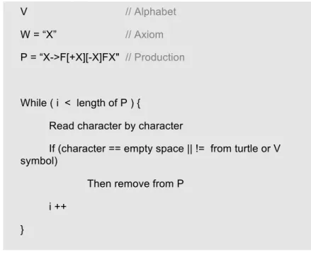
The DOSystem is the simplest of all the different types of L-Systems. It uses a tuple G = <V, w, P>, which consists of:
• V (the alphabet) the set of variables;
• ω (the axiom or word) is the equation defining the initial state of the system, formed by symbols of V;
• P is the set of production rules, or productions, defining how the variables will be replaced by the combinations of symbols. The productions consist of a predecessor and a successor.
The process starts by picking the word and replacing the symbols within it according to the rules defined in the productions. Once all the productions have been applied, the axiom will become a new word and the process can repeat itself. Each replacement step is an iteration which represents a different point in time as the system grows and develops (Grubert, 2001; Prusinkiewicz & Lindenmayer, 1990, 1996; Prusinkiewicz et al., 1988; Bonfim & Castro, 2005; Onishi et al., 2003; Prusinkiewicz, 1997).
Fig.3 – Example of DOL system. Adaptation from Prusinkiewicz & Lindenmayer, 1990 As can be observed in the example shown in Figure 3, the initial word invokes the first production, but in the second iteration there has been the replacement of both symbols in a single step. This illustrates the parallelism feature typical in l-systems, mimicking nature in the sense of several changes happening in different places in the same time. (Grubert, 2001; Envall, 2007; Bonfim & Castro, 2005; Prusinkiewicz et al., 1988).
Unlike the Chomsky grammar, a formal language similar to the l-systems, terminals (symbols that can’t be replaced) and non-terminals (symbols that can be replaced) are not used in l-systems. This is because there isn’t a final goal to be reached. (Prusinkiewicz & Lindenmayer, 1990, 1996; Prusinkiewicz et al., 1988; Grubert, 2001; Bonfim & Castro, 2005). Also, because all words produced are valid models, the empty word λ can be used in a production. As long as all the symbols belong to the alphabet V, they are valid (Grubert, 2001; Bonfim & Castro, 2005; Prusinkiewicz et al., 1988). V: aR, aL, bR, bL w: aR P1: aR → aLbR P2: aL → bLaR P3: bR → aR P4: bL → aL aR aLbR bLaRaR aLaLbRaLbR …
2.2.2 Graphical Interpretation
2.2.2.1 Tree Structure
One interesting aspect of the l-system word is that it can be interpreted as a tree structure. Each symbol represents a node and by reading the word from left to right, with the left-most symbol being the root, we obtain a structure reminiscent to real plants (Prusinkiewicz & Lindenmayer, 1990, 1996; Grubert, 2001; Envall, 2007; Prusinkiewicz et al., 1988). These structures will be very much like straight lines, unless we use the branching structure so well known in plants. To achieve that we need to use two additional symbols, the square brackets to define the beginning and end of a branch V’ = V ∪ { [ , ] } (Grubert, 2001; Envall, 2007; Prusinkiewicz et al., 1988).
When the open bracket ( [ ) occurs the values of the current node and hidden parameters are stored, as well as the position where it occurred. The word is drawn normally until another open bracket or the corresponding closing bracket ( ] ) occurs. When the bracket closes the stored values for that bracket pair are then returned and replace the previous ones. The rest of the tree is drawn from that saved point and the section that was enclosed by the brackets is a sub-tree that sticks out much like a branch from the main trunk (Grubert, 2001; Envall, 2007; Fuhrer, 2005).
Fig.4 – Example of tree representation of the word “A [+ B] [C [D] E] F”. Adaptation from figure 1 of Grubert (2001).
2.2.2.2 Turtle Representation
Although the tree structure helps visualizing the l-system word, it doesn’t give a clear idea of the appearance of the model. In order to have a full idea of their appearance the LOGO turtle graphics are used (Grubert, 2001; Prusinkiewicz & Lindenmayer, 1990, 1996; Prusinkiewicz et al., 1988; Fuhrer, 2005).
The turtle is a cursor that moves and rotates in a Cartesian coordinate system, depending on the instructions given and the defined angle. Examples of some of the commands are (Grubert, 2001; Prusinkiewicz & Lindenmayer, 1990, 1996; Prusinkiewicz et al., 1988; Envall, 2007; Fuhrer, 2005; Onishi et al., 2003):
F : Move forward a unit and draw a line from the last
position to the current one;
f : Move forward a unit, without drawing a line; + : Rotate the cursor counter-clockwise by angle α; - : Rotate the cursor clockwise by angle α.
Fig.5 – Example of a turtle representation of a L-System. Adaptation from figure 2 of Grubert, (2001)
As it can been seen in the example shown in Figure 5, each iteration replaces each unit of the previous one with the whole structure previously generated, creating a model with increasing detail. This happens as each predecessor (in this case just one) is replaced by its correspondent successor (Prusinkiewicz & Lindenmayer, 1990, 1996; Prusinkiewicz et al., 1988; Envall, 2007; Chen et al., 2003; Onishi et al., 2003).
Values like angles and unit length are hidden parameters. They are set before the iterations take place and do not change as they go (Envall, 2007; Prusinkiewicz et al., 1988).
2.2.3 Parametric L-Systems
A problem with the DOL system is that when you need to use different sizes or angles, it’s necessary to find a denominator common to all and combine several transformation symbols to achieve a certain rotation or translation (Grubert, 2001; Prusinkiewicz & Lindenmayer, 1990, 1996).
The Parametric L-System allows adding different parameters to different symbols. These parameters can be used to store information about the model from age and size to angle and time (Grubert, 2001; Envall, 2007; Prusinkiewicz & Lindenmayer, 1990, 1996; Prusinkiewicz & Hanan, 1990; Prusinkiewicz, 1997).
Fig.6 – Example of a Parametric L-System. Adaptation from Grubert (2001)
V: { A } w: A (2)
P1: A (a): a > 0 → A (a – 1)
Pa: A (a): a <= 0 → λ
As can been seen in the example shown in Figure 6, the symbol is followed by the parameter. Like in the DOL system, every time the productions occur the value is replaced accordingly, though the conditions have to be fulfilled for the value to be altered (Prusinkiewicz & Lindenmayer, 1990, 1996; Grubert, 2001; Envall, 2007; Fuhrer, 2005; Prusinkiewicz, 1997).
In the turtle interpretation, in order to draw the model the operators used are a bit different from the ones used in DOL systems (Envall, 2007; Bonfim & Castro, 2005; Prusinkiewicz, 1997):
F(a) : Move forward a unit of length a > 0 and draw a line from the last position to the current one;
F (a) : Move forward a unit of length a > 0, without drawing a line +(a) : Rotate the cursor by angle a. Counter-clockwise if a is positive, clockwise if negative.
Fig.7 – Example of a Parametric L-System. Adaptation from figure 1.40 from Envall (2007)
2.2.4 Context-Sensitive L-Systems
Up until now we’ve only seen context free systems (OL-Systems), systems that don’t take into consideration the context its predecessor is in, but any living organism suffers influence from its surrounding environment which affects its growth.
The Context-Sensitive L-System takes into consideration the different interactions between the different sections of the word by verifying what’s happening on the right and left of the said symbol (Prusinkiewicz & Lindenmayer, 1990, 1996; Prusinkiewicz et al., 1988; Envall, 2007 Bonfim & Castro, 2005; Fuhrer, 2005).
Fig.8 – Example of a Context-Sensitive L-System. Adaptation from Prusinkiewicz & Lindenmayer (1990)
As you can see in Figure 8, the productions use the < and > brackets to check what is happening on the left and right context, respectively. It’s not mandatory to check both sides, as illustrated in the second production, but in either case the production will only be applied if the specified context occurs. (Grubert, 2001; Prusinkiewicz & Lindenmayer, 1990, 1996; Prusinkiewicz et al., 1988; Envall, 2007; Chen et al., 2003).
In the example from Figure 8 the first production checks if there’s a symbol A on the left and a symbol C on the right of the symbol B. In case that’s true then the symbol B takes the value n in A and replaces its own with it. The second production only checks if there’s a symbol B on the left of C, but the sucessor will only occur when the condition is true.
In the situation where both context-free and context-sensitive productions are used and both applied on the same letter, the context-sensitive has priority over the context-free production. However, if neither occurs, then the letter is replaced by itself (Prusinkiewicz & Lindenmayer, 1990, 1996; Envall, 2007).
V: { A, B, C } w: A(5) B(0) C(0)
P1: A(n) < B > C: true → B(n)
Pa: B(n) < C: n > 2.5 → C(n – 2)
The [ and ] brackets make it harder to keep track of the context, because the branches they specify don’t preserve the segment neighborhood. Therefore, it’s often necessary to skip the information contained within them to verify the context of the other symbols (Prusinkiewicz & Lindenmayer, 1990).
Below is an example of a word where the predecessor BC < S > G [ H ] M is valid to the symbol S, because it skips over the symbols [ DE ] to look for the left context and the I [ JK ] L to search for the right one.
ABC [ DE ] [ SG [ HI [ JK ] L ] MNO ]
In the turtle interpretation the + and – symbols are ignored when verifying the context in the word (Prusinkiewicz & Lindenmayer, 1990, 1996).
Fig.9 – Example of Context-Sensitive L-Systems. Adaptation from figure 1.31 from Prusinkiewicz & Lindenmayer (1990).
2.2.5 Stochastic L-Systems
All of the L-Systems seen so far are deterministic in nature. No matter how many times they are run, as long as the word and the productions stay unchanged, the result is always the same. In some situations this might not be a good option.
The Stochastic L-Systems introduce a variation from individual to individual, but does not alter the general information of the species. This is done by introducing a probability value that will determine which production will be used (Grubert, 2001; Prusinkiewicz & Lindenmayer, 1990, 1996; Chen et al., 2003).
Fig.10 – Example of a Stochastic L-Systems. Adaptation from figure 3 from Grubert (2001).
As can been observed in the example presented in Figure 10, the probability for each of the productions to occur is written in front of the arrow, though in some cases it’s written on top, where the sum of the probabilities is 1 (Grubert, 2001; Envall, 2007). During the iterations, if more than one production occurs on the same symbol a random number is generated to select one of them, based on their assigned probabilities (Grubert, 2001; Envall, 2007).
Fig.11 – Example of a Stochastic L-Systems. Adaptation from figure 1.27 from Prusinkiewicz & Lindenmayer (1990)
V: { F, +, -, [, ] } w: F
P1: F →0.33 F [+F] F [-F] F
P2: F →0.33 F [+F] F
2.3 Genetic Programming
The theory of evolution proposed by Charles Darwin in 1882 (Cited in Russell & Norvig, 2004; Azevedo et al., 2005), in which natural selection plays a crucial role in the species evolution, is by far the best model which can explain the wide variety of life in our planet (Darwin, 1859, cited in Russell & Norvig, 2003). The theory has evolved, with the aid of new discoveries, such as genes, which has filled many of the gaps that Darwin struggled to explain during his time, but the theory itself is in constant evolution (Darwin, 1859, cited in Russell & Norvig, 2003).
Natural Selection is a process that favours certain individuals in a population in order for a species to evolve (Russell & Norvig, 2004; Azevedo et al., 2005; Vega, 2001).
Each individual carries genotype and phenotype information. Genotype is the type of genes it carries, all the information it inherited from its parents and the information its offspring will inherit from it. Phenotype is its physical attributes, like weight for example, and they determine its survival and reproduction chances (Peterson, 1997, Azevedo et al., 2005; Vega, 2001). These traits determine the ability of an individual to survive in its environment. Those with more favourable traits are more likely to survive and pass on their heritage than those with less favourable attributes: this is the survival of the fittest principle. As new generations keep evolving and continuously adapting to their ever changing environment, there’s the chance new species may emerge as they take different ecological niches (Peterson, 1997, Azevedo et al., 2005; Vega, 2001).
Evolutionary Algorithms, in which Genetic Programming is a particular branch, take advantage of this highly powerful mechanism and try to simulate it in a computer. This will be explained further below.
2.3.1 Evolutionary Approaches
The power of nature has always marvelled humanity, but only in the last few centuries has mankind truly tried to understand and harvest its potential. The creation of velcro, the invention of the airplane, all of these ideas were inspired by models that existed in nature for ages (Vega, 2001).
The same happens in Evolutionary Computation. This subfield of Computacional Intelligence takes inspiration from biological evolution and natural selection to optimize possible solutions and solve a given problem (Morais, 2003; Coello, 2007; Pappa & Freitas, 2006; Vega, 2001)
Fig.12 – Evolutionary Computation Index. Adaptation from figure 1 of Morais (2003) As shown in Fig.12, the Evolutionary Computation branches into five different subfields: Genetic Algorithms, Evolutionary Programming, Evolution Strategy, Learning Classifier System and Genetic Programming. All of them share the same evolutionary nature but take different approaches when it comes to its implementation (Morais, 2003; Coello, 2007; Pappa & Freitas, 2006).
2.3.1.1 Genetic Algorithms
The most popular of the Evolutionary Algorithms, Genetic Algorithms, use the mechanisms of natural evolution, such as selection, crossover, mutation and fitness evaluation,and apply them to a population of individuals (Morais, 2003; Coello, 2007; Vega, 2001).
Each of the individuals (in a canonical GA) has a fixed size and is usually represented by an array of bits, in analogy to chromosomes in DNA. One of the advantages of that representation is the simplicity of the crossover operator, though it’s possible to use arrays of different sizes, but that increases the level of complexity (Morais, 2003; Coello, 2007; Vega, 2001).
Fig.13 – Example of a Genetic Algorithm. Adaptation from figure 2 of Morais (2003). Begin {
t = 0; // Initialization of time
initPop P(t); // Initialization of Population
fitnsEval P(t); // Evaluation of the Initial Population
While (solution not reached) {
t ++; // Incrementation of time
P’ = selctParent P(t); // Select parents of future generation
crossover P’(t); // Breed parents
mutate P’(t); // Add diversity to generation
evaluate P’(t) ; // Evaluate fitness of generation
P = survive P,P’(t); // Replace population
} }
2.3.1.2 Evolutionary Programming
Evolutionary Programming shares a lot of similarities to Genetic Algorithms, but it pays more attention to the behavioural relationship between parents and offspring, instead of mimicking the genetic operators found in nature (Morais, 2003; Coello, 2007).
The main difference in the implementation method is not using the crossover operator but relying on mutation and fitness to determine the survival. Another difference between evolutionary programming and Genetic Algorithms is the use of graphs instead of arrays in the solution representation (Morais, 2003; Coello, 2007).
Fig.14 – Example of an Evolutionary Programming algorithm. Adaptation from figure 3 of Morais (2003).
Begin {
t = 0; // Initialization of time
initPop P(t); // Initialization of Population
fitnsEval P(t); // Evaluation of the Initial Population
While (solution not reached) {
P’ = mutate P(t); // Add diversity to Population
evaluate P’(t) ; // Evaluate fitness of generation
P = survive P,P’(t); // Replace population
t ++; // Incrementation of time
} }
2.3.1.3 Evolution Strategy
The Evolution Strategy works with vectors of real numbers to represent solutions. Its approach is for each parent to produce an offspring per generation by the use of mutations. It’s more likely for the evolution to occur in smaller steps until the descendent shows a better performance than its parent, replacing it (Morais, 2003; Coello, 2007).
Fig.15 – Example of an Evolution Strategy algorithm. Adaptation from figure 4 of Morais (2003).
Begin {
t = 0; // Initialization of time
initPop P(t); // Initialization of Population
fitnsEval P(t); // Evaluation of the Initial Population
While (solution not reached) {
P’’(t) = selectBest (a, P(t)); // Select best parents
P’(t) = crossover (b, P’’(t)); // Breed parents
mutate P’(t); // Add diversity to generation
evaluate P’(t) ; // Evaluate fitness of generation
if (usePlusStrategy)
P (t+1) = P’(t) ∪ P(t); // Child joins Population
else
P (t+1) = P’(t); // Population remains same
t ++; // Incrementation of time
} }
2.3.1.4 Learning Classifier System
The Classifier System doesn’t use a fitness function to evaluate the individuals, but a rule based on a reinforcement learning technique (Morais, 2003; Coello, 2007). This technique works by setting the program on an environment about which it has no knowledge and through a set of actions provided, reacts and classifies the environment as it changes. The Classifier System, specifically, has a population of binary rules on which a special genetic algorithm selects the best ones (Morais, 2003; Coello, 2007).
Fig.16 – Example of Learning Classifier System rules. Adaptation from figure 5 of Morais (2003).
2.3.1.5 Genetic Programming
Genetic Programming is very similar to Genetic Algorithms, to the point that some authors consider it a subtype (Coello, 2007). The main difference is that in Genetic Programming individuals are represented as a tree instead of an array or string. Actually, they’re not a string of characters, but programs, thanks to the way of defining information (Morais, 2005; Peterson, 1997; Coello, 2007; Pappa & Freitas, 2006; Vega, 2001).
// Takes decisions by If-then rules
(1) If (ship is left) then send @ (2) If (ship is right) then send % (3) If (ship is centre) then send $ (4) If (ship is attacking) then send # (5) If (ship is not attacking) then send *
(6) If (* and @) then don’t set cannon (7) If (* and %) then don’t set cannon (8) If (* and $) then set cannon (9) If (#) then fire cannon
The array representation has some limitations the tree-based structure can overcome. Because of their rigid nature, they’re not suitable to represent arbitrary computational procedures or to incorporate iterations or recursion within the individual. Also, their fixed size doesn’t allow much dynamic variability being the string length given in the initial population (Koza, 1990, 1992, 2001, 2007).
Fig.17 – Example of a Genetic Program. Adaptation from Algorithm 2.2 fig of Peterson, 1997.
t = 0; // Initialization of time
initPop P(t); // Initialization of Population
fitnsEval P(t); // Evaluation of the Initial Population
While (solution not reached) {
t ++; // Incrementation of time
if (reproduce) {
P’ = selctProg P(t); // Select individual programs
} else {
if (recombine) {
P’ = selctParent P(t); // Select parents
crossover P’(t); // Breed parents
} }
mutate P’(t); // Add diversity to generation
evaluate P’(t) ; // Evaluate fitness of generation P = survive P,P’(t); // Replace population
2.3.2 Operators
According to Koza, the creator of Genetic Programming, the algorithm can be divided into two major operators and five minor ones (Koza, 1990, 1992, 2001, 2007). The two major operators are reproduction and crossover, the fundamental forces behind evolution (Peterson, 1997; Koza, 1990, 1992, 2001, 2007; Vega, 2001).
The five minor ones are mutation, permutation, editing, encapsulation and decimation. Usually, only mutation is used and sometimes editing and encapsulation as well, while permutation and decimation are quite rare (Peterson, 1997; Koza, 1990, 1992, 2001, 2007; Vega, 2001).
Koza defends that the two major operators are enough to have a working Genetic Program, but the minor ones may be used to provide extra functionality (Peterson, 1997; Koza, 1990, 1992, 2001, 2007).
2.3.2.1 Individuals and Initial Population
As stated before, individuals in Genetic Programming are programs organized in a tree structure. Their shape, size and complexity change dynamically during the evolutionary process, but because individuals are represented in a tree hierarchy, the initial population generation is more complex than in Genetic Algorithms (Peterson, 1997).
Instead of a randomly generated number, a correct tree structure has to be created. Each tree is created individually with a single function as the root and has a predefined tree depth maximum value to balance the weight of the branches (Peterson, 1997; Koza, 1990, 1992, 2001, 2007; Vega, 2001). This is important
during the crossover in order to prevent unwanted individuals from being generated.
Fig.18 – Generating a Random Program. Adaptation from Algorithm 2.3 fig of Peterson, 1997.
// F = {f1, f2, …, fn}; set of functions
// T = {t1, t2, …, tn}; set of terminals
Randomly select a function root ∈ F If (depth = depthmax – 1) {
Randomly select a terminal ∈ T }
else {
if (root is a function) {
for (argj , j = 1,…, φ(root)) {
φ(f) = the parity of f if (use grow method) {
Randomly select argj ∈ F ∪ T
} else {
if (use full method) {
Randomly select argj ∈ F
} }
Recursively generate subtree with argj as root
} }
else {
root is a terminal }
This branch is complete }
Figure 18 shows the generation of an individual. Koza defines two different variations, the Grow and the Full methods. The Grow generates trees of random size and shape while the Full produces them with uniform size and shape. However, in order to ensure diversity, he uses a hybrid version of the two methods, called Ramped Half and Half method (Koza 1990, 1992, 2001, 2007; Peterson, 1997; Vega, 2001).
The maximum tree depth is ramped according to the size of the population. In a population of size N, the subpopulation will be of size N/2 (Peterson, 1997; Vega, 2001).
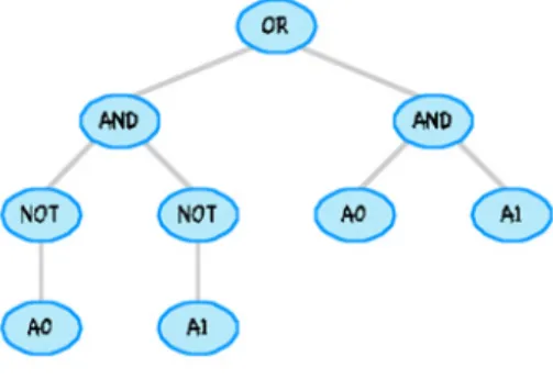
Fig.19 – Example of an Individual. Adaptation from fig.11 of [18]
Individuals may contain arithmetic operations (e.g. =, -, x, /), mathematical functions (e.g. sine, exponential, logarithms), Boolean operations (e.g. AND, OR, NOT), logical operators (if-then-else, etc), iterative operators (while-do, etc), recursive functions, among others. It all depends on the problem in cause. These will be the functions defining the body of the program (Koza, 1990, 1992, 2001, 2007; Coello, 2007; Pappa & Freitas, 2006; Vega, 2001).
The terminals can be constant atomic arguments (state variables of a system for example), constant atomic values (0, 1, etc) and even other atomic entities, like functions with no arguments (Koza, 1990, 1992, 2001, 2007; Pappa & Freitas, 2006; Vega, 2001).
When defining the set of functions and terminals for a specific problem, it’s necessary to satisfy the conditions of closure and sufficiency. Closure requires that any function used can accept any value and data type returned by any other function or terminal (Peterson, 1997; Pappa & Freitas, 2006), which guarantees the validity of the program. In order to do this it might be necessary to use functions that return default values (for example, if a value is divided by zero, the function returns a default value instead of an unidentified situation).
Sufficiency requires that the given problem solution exists within the search space by using functions and terminals (Peterson, 1997; Pappa & Freitas, 2006).
2.3.2.2 Fitness
The fitness function (objective function) evaluates the aptitude of survival of the individuals in the population and it is an indispensable tool for the Genetic Programming to work. The fitness function analyses how much a potential solution can satisfy the problem (Peterson, 1997; Koza, 1990, 1992, 2001, 2007; Pappa & Freitas, 2006).
The fitness function varies according to the problem at hand, since most optimal solutions have to be calculated with different formula. But all fitness functions try to determine which individuals of the population of possible solutions is closer to the optimal result. For example, on a broom balancing problem, the smaller the time it takes to balance the broom and the longer it stays balanced, the better the fitness of that individual (Koza, 1990, 1992, 2001, 2007; Vega, 2001).
It’s important that the value the fitness function returns gives enough information of how fit the individual is. For example, if it only returns either 0 or 1, the performance of the individual can’t
be evaluated correctly, especially in later cases where the fitness values are higher and therefore more similar (Koza, 1990, 1992, 2001, 2007).
However, if the problem requires a subjective judgement, like evaluating the aesthetic quality of an image, then it may be very difficult to define the fitness. To solve this problem an outside source, as a user, replaces the fitness function and determines which members of the population are more suitable for reproduction. In some cases the selection is done directly, while others filter part of the population beforehand (Peterson, 1997). This interactive evolution system is best for small populations. There are many limitations the human comprehension forces upon this, such as inability to pick minor variations in the representation or not being able to deal with many individuals at the same time (Peterson, 1997). Usually the magnitude of individuals to be picked is less that 25, which reduces the diversity of the population greatly. Because of the sall population size high mutation rates are often used to compensate the lack of diversity (Peterson, 1997).
2.3.2.3 Reproduction
This genetic operator combines the information contained by parents to create an offspring. In the natural world the same happens when a chromosome pair recombines to generate a new DNA strand (Peterson, 1997; Coello, 2007).
Before the parents information is recombined, they are both selected based on the same fitness criteria. Depending on the approach to solve the problem, we can either have an asexual or sexual reproduction and reselection might or might not be allowed (Peterson 1997; Koza, 1990, 1992, 2001, 2007).
An asexual reproduction only involves one parent to generate an offspring. Several individuals of the population are selected based on their fitness (which evaluates their performance) and the probability of reproduction (which defines how many can reproduce) (Peterson, 1997).
The offspring that will form the new population are clones of their parents. As a result of that, reselection is allowed in this case (Peterson, 1997; Vega, 2001).
Sexual reproduction, also known as Crossover, recombines the genetic information of the parents to generate an offspring. The parents are selected in the same fashion as in the asexual reproduction, based on their fitness and crossover probability (Peterson 1997; Koza, 1990, 1992, 2001, 2007; Coello, 2007; Vega, 2001).
Usually in Genetic Programming the crossover is done by using the tree nature the individuals possess and numbering the tree nodes by their reading order (Coello, 2007; Vega, 2001). First, a point is chosen randomly in both trees. Second, the subtrees rooted on those points are selected and detached from the parent trees. Third and finally, the subtrees are switched between the parents, generating a pair of offspring (Coello, 2007; Peterson 1997; Koza, 1990, 1992, 2001, 2007; Vega, 2001).
Note that the resulting offspring from any crossover points are always valid programs, because their parts are taken from the parents, which were also valid expressions (Koza, 1990, 1992, 2001, 2007). The reason for this to happen is because of the closure and sufficiency requirements imposed when the population was first created.
Fig.20 – Crossover example. Adaptation from fig.2.6 of Peterson (1997)
It’s also possible for the root of the trees to be selected, either in one or both parents. If only one root is selected, the entire parent will be copied onto the second, while the subtree of the second parent will become the full tree of the first one (Koza, 1990, 1992, 2001, 2007). If the roots of both parents are selected as crossover points, the children will be copies of their parents, as in a reproduction and not a crossover (Koza, 1990, 1992, 2001, 2007).
In the case of a terminal and a root being selected as crossover points, this often increases the size of one of the trees dramatically (Koza, 1990, 1992, 2001, 2007; Coello, 2007). In order to prevent memory problems, Genetic Program usually imposes a limit on the maximum depth of a tree.
Compared to the Crossover operator in Genetic Algorithms, there are two main differences from the one used in Genetic Programming. First, in standard Genetic Algorithms offsprings have the same size as their parents, no matter the number of generations. In Genetic Programming there’s a big chance of
different sizes and shapes to be formed because of the random crossover points (Peterson, 1997; Coello, 2007).
Second, if reselection is allowed, and individual with high fitness may be chosen to act as both parents, incestuous offspring result. In Genetic Algorithms an incestuous crossover degrades the quality of the offspring to an asexual reproduction. In Genetic Programming the two offspring will likely be different, unless the same crossover points are chosen in both parents (Peterson, 1997; Koza, 1990, 1992, 2001, 2007; Coello, 2007).
2.3.2.4 Mutation
Occasionally a random change will occur during the genes recombination, resulting on a slight mutation that brings variation and new possibilities in the process of evolution.
In Genetic Programming, mutation works by randomly picking a point in the tree and replacing it with a new randomly generated subtree. A probability based on the tree’s depth can prevent excessive terminal swapping or encourage bigger or smaller tress to be produced Peterson, 1997; Coello, 2007; Vega, 2001).
Mutation is very good to add variety and keep the population from becoming stagnated, but it might damage or render a program non functional (Peterson, 1997). It’s possible to protect a certain subtree, known as a good building block, by using encapsulation. The subtree is replaced by a symbolic name that points to its real location (Coello, 2007).
Editing is another operator which helps protecting the tree. Like mutation it replaces certain subtrees with new information, but instead of using a new random subtree, it cleans up the existing one by replacing a constant valued subtree with its corresponding value. For example, (1 (+ 1)) would be replaced by the terminal 2 (Peterson, 1997). This helps avoiding waste of memory and unnecessary depth of the tree, but this parsimony can be harmful to the diversity of the population (Peterson, 1997).
2.3.2.5 Termination Criteria
The evolutionary process ends when the population reaches the solution to the problem, or gets as close to it as possible. There are many different criteria that can be used to define when the whole process terminates, including number of generations, lack of increase of fitness within the population after a certain number of generations, etc (Koza, 1990, 1992, 2001, 2007).
Once that step is reached, the best individual of the whole population is considered the optimal solution to the given problem (Koza, 1990, 1992, 2001, 2007).
There are some cases where outside factors might force the program to end before the optimal solution is found, such as: time, resources and funds.