Predictive models of probability of default : an empirical application

MASTERS OF SCIENCE IN

F

INANCE

MASTERS FINAL WORK

D

ISSERTATION

P

REDICTIVE MODELS OF THE PROBABILITY OF DEFAULT

:

A

N

E

MPIRICAL

A

PPLICATION

J

OÃO

M

ANUEL

N

UNES

C

AETANO

MASTERS OF SCIENCE IN

F

INANCE

MASTERS FINAL WORK

D

ISSERTATION

P

REDICTIVE MODELS OF THE PROBABILITY OF DEFAULT

:

A

N

E

MPIRICAL

A

PPLICATION

J

OÃO

M

ANUEL

N

UNES

C

AETANO

S

:

P

D

.

J

A

R

F

B

i

Abstract

This study intends to conduct a survey of Probability of Default models to listed companies. The methodologies of Merton (1974) model, Accounting model and Hybrid were addressed. We tested a sample of 172 American companies in the sectors of Consumer Products, Distribution, Manufacturing and Telecommunications in which 82 entered into default. For each methodology, the predictive ability was tested with Type I and II errors. The results suggests that the Hybrid model, i.e. a combination of market models and accounting analysis, have a better performance in the classification of credit default than each model individually.

Keywords: Merton; Credit Risk; Accounting Model; Hybrid Model; Black-Scholes;

ii

Resumo

Este estudo tem como objetivo realizar uma pesquisa dos modelos de previsão do incumprimento a empresas listadas em bolsa. Foram abordadas as metodologias do modelo de Merton (1974), modelo Contabilístico e Híbrido. Testou-se uma amostra de 172 empresas presentes no mercado Americano dos setores do Consumo, Distribuição, Produção e Telecomunicações nas quais 82 entram em incumprimento. Para cada metodologia, a capacidade preditiva foi testada através dos erros Tipo I e II. Os resultados sugerem que o modelo Híbrido, i.e., a combinação de modelos de mercado e análise contabilística, confere maior poder de precisão na classificação de incumprimento, ao invés de cada modelo individualmente.

Palavras-Chave: Merton; Risco de Crédito; Modelo Contabilístico; Modelo Híbrido;

iii

Acknowledgements

I am grateful to my supervisor Professor João Bastos, for his detailed and constructive comments in all phases of this thesis.

To complete my study, and without whom it would not be possible this moment, I am also grateful:

To Professor Valentina Valente, for English review,

To my mother, for her support and comfort over the difficult moments, To my father, for his care,

To my grandmother and my aunt, for helping me all these years in Lisbon, To my grandparents António and Rosário, for their concern,

To my brothers and recently born nephew António, for the joy they give me, To my friends Manuel and Helena for their suggestions to the study,

To all my friends, for the fellowship over the years,

To all mentioned and many others not named, thank you very much for your support and for believing in me.

iv

Table of Contents

v

4. Description and Data Treatment ... 19

4.1 Sample ... 19

5. Implementation, Analysis and Results ... 20

5.1 Merton Model Approach ... 20

5.1.1 Default Probability ... 20

5.2 Accounting Model ... 23

5.3 Hybrid Model ... 25

6. Conclusions, Limitations and Future Research ... 29

7. Appendix ... 30

vi

List of Tables

Table 1. Summary of Companies Included in the Study (by Sector) ... 19

Table 2. Omnibus Tests of Merton Model Coefficients ... 21

Table 3. Merton Model Summary ... 22

Table 4. Classification Table between Defaulted and Non-defaulted Companies (with Merton model) ... 22

Table 5. Variables in the Equation (with Merton model) ... 22

Table 6. Economic-financial Ratios Used in the Estimation of the Models ... 23

Table 7. Omnibus Tests of Accounting Model Coefficients ... 24

Table 8. Accounting Model Summary ... 24

Table 9. Classification Table between Defaulted and Non-defaulted Companies (with Economic Financial Ratios)... 24

Table 10. Variables in the Equation (with Economic Financial Ratios) ... 25

Table 11. Omnibus Tests of Hybrid Model Coefficients ... 26

Table 12. Hybrid Model Summary ... 26

Table 13. Classification Table between Defaulted and Non-defaulted Companies (with Hybrid Model) ... 26

Table 14. Variables in the Equation (with Hybrid Model) ... 27

Table 15. Summary of Models’ Predictive Accuracy ... 28

1

1. Introduction

Evaluating the performance of companies and their ability to pay off their debt is a fundamental activity for commercial banks. An essential ingredient of this activity consists of measuring the credit risk of loans due to the uncertainty of the counterparty to fulfill its obligations. The creditworthiness of a company affects its cost of capital and credit spreads. In a credit transaction it is necessary to estimate the components that affect the credit risk of a borrower: the probability of default; the exposure at default; and the recovery rate. This study addresses the problem of evaluating the probability of default. A popular technique for forecasting defaults are the accounting models (see, e.g. Beaver, 1966; Altman, 1968; Ohlson 1980). These models evaluate the creditworthiness of borrowers through accounting and financial ratios, and usually provide satisfactory results. A different approach, that has revolutionized the way that the probability of default is measured, was proposed in the seminal paper of Merton (1974). This is a structural model, using the concept of a call option where the strike price is the debt of the company, and the price of the underlying asset is the company's assets. A shortcoming of these models is that they can only be implemented for listed companies. Nevertheless, structural models have been the subject of various developments over the years (see, e.g. Moody’s KMV model).

In a recent study, Tudela and Young (2003) suggest combining a structural model with an accounting model to obtain better accuracy in forecasting defaults. This “hybrid” model showed a very good performance. The objective of this study is to replicate this finding using an original data set. This data set was constructed using information from Moody’s Ultimate Recovery Database and Datastream. It is shown that a hybrid model resulting from the combination of a structural model and an accounting model does indeed give better accuracies with respect to the individual models.

The remainder of this study is organized as follows. Chapter 2 presents a literature review. Chapter 3 describes the framework of the models used in this study: the structural and the accounting models. Chapter 4 describes the data used in the empirical work. The

2

forecasting accuracies, such as type I1 _{and II}2 _{errors, are reported and discussed in} Chapters 5. Finally, Chapter 6 provides some concluding remarks.

1 _{Type I error: error of rejecting the null hypothesis when it is true. In other words, it means classifying a}

company as 'defaulted' when it is 'non-defaulted'.

2 _{Type II error: error of not rejecting the null hypothesis when it is false, i.e., classifying a company of}

3

2. Literature Review

Several articles explore models of credit analysis to companies, but not all reach the same conclusion. Therefore, this section aims to review some types of credit analysis models such as structural, the reduced form, accounting based and hybrid models.

In 1968 and most recently in 2000, Altman presents a model of accounting analysis to evaluate the probability of bankruptcy of companies. This is a traditional approach where the author uses five financial ratios to evaluate companies’ health.

On the other hand, in recent years several authors have attempted to assess the default risk of companies using models based on the theory of options, the Black Scholes (1973) model. This is the case of Merton (1974) which is a structural one. Although several authors refer that this type of model presents quite significant predictions, others consider the opposite stating that traditional (i.e. Altman Z-score and Ohlson's O-score) models can provide better information of the state of enterprises. Apart from structural models, reduced form models have been developed. These models introduce explicit assumptions regarding the dynamics of the variables of default which are modeled independently from the structural characteristics of the enterprise.

2.1 Merton Model (1974)

According to the literature, there are several advantages of using structural models. Sundaram (2001) states that the fact that being a model based on economic information adds value because it uses information from market prices and the incorporation of equity prices makes it a prospective model (as opposed to models based on accounting information). He claims that the model appears to have some predictive power for default and ratings transition.

On the other hand, the model has several assumptions that are mostly infringed in practice. From the structure of the capital, where if it is too complex the application of the model can become extremely challenging, as Sundaram (2001) and Elizalde (2005) mentioned.

4

Elizalde (2005) presents in its paper a guide to the literature on Merton (1974) suggesting possible extensions in the model for future development. The author states that one of the problems of the Merton’s model is the time restriction until maturity of the debt default. For instance, in the original model it is not possible that failure happens before maturity. Leland (2002) examines the differences in default probabilities generated by two types of structural models. In the first group, called the 'exogenous default threshold' approach, Merton (1974) and Black and Scholes (1973) models are used. According to the author, the model works for long-term horizons, albeit for short maturities the predictive default frequency is low. In addition, endogenous models predict a rise in the probabilities of failure with the costs of default and a decrease with the maturity of the obligation, unlike the default probabilities derived from exogenous models which do not vary under these parameters.

Huang and Huang (2002) propose a calibration approach based on historical data on defaults. They show that one can obtain consistent estimates of credit spreads through various economic considerations through a structural framework for the assessment of credit risk.

Vassalou and Xing (2004), as a way to realize the effect that the default risk has on stock returns, have conducted a study to assess default probabilities for individual companies using the Merton (1974) model. They concluded that both the size and the book-to-market have a strong impact on default risk.

On the other hand, Jarrow (2011) argues that structural models are not useful neither for pricing nor risk management due to inconsistency with the balance of the credit market. As a result, he states that structural models are not useful to infer default probabilities. Hamilton, Sun and Ding (2011) compare a point-in-time (PIT) and a through-the-cycle (TTC) structural models. A PIT uses all available and pertinent information in a given date to estimate a firm’s expected probability of default over some time horizon. This model is very reactive to all news affecting the firm but also highly volatile. On the other hand, a TTC reflects a firm’s long-run, a credit risk trend. They argue that a complete credit risk management system requires both PIT and TTC credit risk measures.

5

2.2 KMV-Merton Model

Crosbie and Bohn (2003) state that the most effective way to measure the default derives from models using both market prices and financial statements. In their study, they explain how to calculate the expected default frequency (EDF) with the KMV model. This consists on estimating the market value and volatility of companies assets, calculate the distance to default and turn it into expected default frequency using it for an empirical distribution of defaults.

Wang et al. (2009) study the measurement of credit risk of listed companies using different types of credit risk models such as KMV model. The results show that the KMV model can reflect the risk of default.

Bohn, Arora and Korablev (2005a) validate the performance of the model MKMV EDF in its ability to differentiate good firms from bad firms in North America’s market. They compare the KMV model with other popular alternatives such as rating agencies, Z-scores and the simplest version of the Merton model. Tests indicate that the EDF model MKMV had a good and consistent performance across different time periods and different sub-samples based on the company’s size and credit quality. According to the authors, the MKMV model is superior compared to other alternatives until the date of the study (2005).

Bharath and Shumway (2008) examine the accuracy and the contribution of the Distance to Default model (DD) and conclude that this model is useful in default predictions but they state that it is not statistically sufficient. They also report that the structural models provide a useful guidance to build predictive models of default.

2.3 Reduced-form Models

The main characteristic of a reduced form model is given by two assumptions: an exogenously given process for the firm’s default time; a given process exogenously for recovery. On the word of Jarrow (2011) “these are asymmetric information assumptions”.

6

Jarrow and Turnbull (1995), as a way to change the assumptions of symmetric information of structural models, introduce the reduced form models. Other authors, such as Lando (1998), Jarrow et al. (1997) Duffie and Singleton (1999), have extended these type of models using market prices of companies, i.e. bonds or Credit Default Swaps (CDS), to extract both the probability of default and credit risk dependencies. They assume that the market is the only source of useful information to structure the credit risk companies.

According to Elizalde (2005), the reduced form models require the link between credit risk and the information about the financial situation of companies incorporated in the structure of its assets and liabilities. "A reduced form model, despite not compromising the theoretical question of complete information, suffers from other weaknesses including the lack of a clear economic rationale to define the nature of the infringement procedure." (Arora, Bohn, & Zhu, 2005)

One advantage of the structural models versus the reduced form is the ability to link the company’s value to its probability of default, where reduced-form cannot. Notwithstanding, Arora, Bohn and Zhu (2005) argues that reduced form models are flexible in functional form, which could be a strength and a weakness. However, “this flexibility in their functional form can result in a model with strong engagement of the sample properties but poor predictive abilities outside the sample." (Arora, Bohn, & Zhu, 2005)

Uhrig-Homburg (2002) reports that the reduced form models appear to be ideal for evaluating complex credit derivatives, they easily adapt to different situations and there are several variations that are flexible enough to be calibrated to arbitrary data market. As stated by Teixeira (2011) reduced form models do not condition default on the firm’s value. Hence, the assumptions about the dynamics of the default variables are modeled independently from the characteristics of the company, asset volatility and leverage. Comparing reduced form models with the structural models, the latter takes into account symmetric information. According to Jarrow (2011), both the management and the market have the same information about the process of asset value. He states that there is no adverse selection or moral hazard in structural models. In contrast, and shown by

7

Jarrow and Protter (2004), reduced models are consistent with asymmetric information in credit markets.

2.4 Accounting Models

We can define the accounting analysis models as retrospective, because they indicate the health of a company at a certain time. According to Beaver (1966) the analysis of financial ratios can be useful to predict bankruptcy up to 5 years before it happens.

Altman’s (1968) accounting analysis model is one of the most popular. He uses five financial ratios to measure the probability of a company enters into bankruptcy, through the Multiple Discriminant Analysis (MDA). According to Ohlson (1980), the MDA presents some problems in predicting business failures: the need for equality of variance-covariance matrices of the predictors of the two groups of companies; intuitive interpretation of the Z-score and the arbitrary nature of the process of matching the sample, since "failed and non-failed companies are categorized according to criteria such as size and industry, and these tend to be of any arbitrary shape." (Ohlson, 1980) Other methodologies have been addressed in the analysis of financial ratios, such as Probit and Logit.

According to Ferrando and Blanco (1998) one of the advantages of the Logit model is the possibility of categorizing the independent variables, admitting not only the economic and financial ratios or metric variables, and allowing the use of non-financial or qualitative information.

Lo (1986) states that, for purposes of parameter estimation, the Logit has been shown to be more robust than Discriminant Analysis. Nevertheless, under certain distributional assumptions both procedures yield consistent estimates. Furthermore, the Logit model has simpler representation and mathematical treatment compared to the Probit one.

8

2.5 Hybrid Models

Sobehart and Stein (2000) use financial statements and market information to build a hybrid model to predict the failure of public companies based on methods of nonlinear regression. According to the authors, "market information provides an overview, and has already proved to be useful in predicting defaults. It also reflects changes in the investors’ preferences not related to the solvency of the company." (Sobehart & Stein, 2000) On the other hand, they argue that the financial statements contain specific information that demonstrates the financial state of the company.

Tudela and Young (2003) developed a hybrid approach to evaluate the default risk of listed companies through a version of Merton's (1974) model with the use of accounting data. The results show that the combination of the accounting data to the default probabilities derived from Merton model produces better results compared to the implementation of each model individually. In the Merton model developed by the authors, a barrier option is used allowing the default to occur at any time rather than specifically at the end of the maturity of debt.

Benos and Papanastasopoulos (2007) combine fundamental analysis with structural analysis in a hybrid model for measuring credit risk. These two authors develop the initial Merton model assuming a more complex structure of capital (adjusted for dividend payments) introducing randomness to the time of default, allowing a fractional recovery at the time of default. Thus, using financial ratios and the distance to the default of the structural model, a hybrid model is estimated through a Probit regression model. Its main conclusion is that the accounting data and financial ratios contain information that provides additional value to the Merton model.

Another type of approach is used by the risk assessment company Kamakura Corporation (2011), with the structural model to evaluate private companies (Merton model), the Jarrow Merton Hybrid model and also the Jarrow Chava model. The latter is a statistical model hazard that includes financial information and ratios of stock market prices. Here the failure can occur at any time during the period of analysis. In Jarrow Merton, a statistical hazard model is used with the same explanatory variables as the Jarrow Chava model and incorporates the Merton structural model as an additional variable.

9

3. Theoretical Framework

3.1 Structural Models

This section describes the model of credit rating companies based on Black and Scholes (1973), the Merton model (1974) and Moody’s KMV. In general terms, this model uses the concept of a call option where the strike price is the debt of the company and the price of the underlying asset is the company's assets, so if this is lower than the value of the debt then the company is considered to enter into default.

According to Cossin and Pirotte (2001), it is considered a structural approach since it depends on the sharing of value between the shareholders and debt holders, which is the structure of the company itself.

One of the constraints of the model is that the assets of the company are neither traded nor observable and to test the model, parameters have to be estimated implicitly. "This creates a strong joint hypothesis in empirical testing of the models." (Jarrow, 2011)

3.1.1 Merton Model (1974)

According to the Merton’s (1974) model of credit analysis, the shareholders of a company by contracting a loan are actually transferring the control of the company to creditors. However, if the liabilities of the company are liquidated we have the ability to retrieve this control, so the value of equity can be seen as the price of an option on assets of the company, with the strike price corresponding to the value of debt.

The model thus assumes that the capital structure of the company comprises equity and a zero coupon bond with maturity 𝑇 and face value of 𝐷, where the values in period t are entitled 𝑉_𝐸 and 𝑧(𝑡, 𝑇) respectively for 0 ≤ 𝑡 ≤ 𝑇. The asset value of the company 𝑉_𝐴 is the sum of equity 𝑉_𝐸 and debt 𝐷 values.

Therefore, equity represents a call option on assets of the company with maturity 𝑇 and strike price of 𝐷. If at maturity 𝑇 the value of the assets of the company 𝑉_𝐴 is insufficient to pay the face value of debt 𝐷 , i.e. 𝑉𝐴 < 𝐷 , then the company goes into default.

10

Otherwise, if 𝑉𝐴 > 𝐷 then the company does not enter into default and shareholders receive 𝑉𝐴− 𝐷.

The assumptions that Merton (1974) adopts are the following:  the company can only default in 𝑇;

 the absence of transaction costs, bankruptcy costs, taxes or problems of indivisibility of assets;

 transaction in continuous time; unrestricted borrowing and lending at a constant rate r;

 no restrictions on short selling of assets;

 the company's value is invariant under changes in capital structure (Modigliani-Miller theorem);

 the company’s asset value follows a diffusion process:

𝑑𝑉𝐴 = 𝑟𝑉𝐴𝑑𝑡 + 𝜎𝐴 𝑉𝐴𝑑𝑊 (1)

Where 𝜎_𝐴 is the asset volatility (relative) and 𝑊 follows a Brownian motion.

The Payoffs of equity holders and bondholders at 𝑇 under the assumptions of this model are respectively, 𝑚𝑎𝑥 {𝑉_𝐴 − 𝐷, 0} and 𝑉_𝐴 – 𝑉_𝐸, i.e.

𝑉_𝐴 = 𝑚𝑎𝑥 {𝑉_𝐴 − 𝐷, 0} (2)

𝑧 (𝑇, 𝑇) = 𝑉_𝐴 − 𝑉_𝐸 (3)

Applying Black-Scholes pricing formula, the value of equity 𝑉_𝐸 at 𝑡 (0 ≤ 𝑡 ≤ 𝑇) is given by:

𝑉_𝐸(𝑉_𝐴, 𝜎_𝐴, 𝑇 − 𝑡) = 𝑉_𝐴𝑁(𝑑₁) − 𝐷𝑒−𝑟(𝑇−𝑡)_𝑁(𝑑

2) (4)

11 𝑑₁ = ln ( 𝑉𝐴 𝐷 ) + (𝑟 + 1 2 𝜎𝐴2) (𝑇 − 𝑡) 𝜎𝐴√𝑇 − 𝑡 (5) 𝑑₂ = 𝑑₁− 𝜎_𝐴√𝑇 − 𝑡 (6)

The probability of default in 𝑇 is given by:

𝑃 [𝑉_𝐴 < 𝐷] = 𝑁(−𝑑₂) (7)

Thus, the value of debt at 𝑡 is equal to 𝑧 (𝑡, 𝑇) = 𝑉_𝐴 − 𝑉_𝐸.

In order to implement Merton’s model, the value of company assets 𝑉𝐴 and its volatility 𝜎_𝐴 must be estimated, transforming the structure of debt the company into a zero coupon bond with maturity 𝑇 and face value of 𝐷.

3.1.2 KMV-Merton Model

The KMV-Merton model was developed by KMV in the late 80s, being successfully marketed by KMV in a successfully manner until it was acquired by Moody's in April 2002.

The basic methodology of this model is discussed in Crosbie and Bohn (2003), Kealhofer (2003a), Vasicek (1984) and Bharath and Shumway (2004).

This model is based on the Merton model (1974) where the major difference lies in the use of an empirical distribution of defaults of companies to transform the Distance to Default and Expected Default Frequency (EDF).

The KMV model considers the company as a perpetual entity, which issues debt on a continuous basis. Secondly, deals with different classes of liabilities, so it is able to better capture details of the capital structure. The model assumes that the company goes into bankruptcy when achieves the Default Point (DPT) and the debt plus half of long term

12

debt to short-term. Lee (2011) indicates that there may be different DPT depending on the country of companies to study.

Like in Merton (1974), in KMV model, the equity of the company is considered as a call option based on the underlying price of the company with a strike price equal to the face value of the debt of the company with time-to-maturity 𝑇. Therefore, the value of equity is a function of the total value of the firm that can be described by the formula of Black-Scholes-Merton.

Here, two particular assumptions are taken. The first is that the value of the asset follows a Brownian motion such that:

𝑑𝑉_𝐴 = 𝜇𝑉_𝐴𝑑𝑡 + 𝜎_𝐴𝑉_𝐴𝑑𝑍 (8)

Where 𝑉𝐴 is the total value of the assets of the company, 𝜇 is the expected continuously compound return 𝑉_𝐴, 𝜎_𝐴 is the volatility of the company and 𝑑𝑍 is a standard Wiener process. The second assumption is that the company just issued a bond that matures in 𝑇. According to the put-call parity, the value of the debt of the company is equal to the risk free discount bond minus the put option written on the company, similarly with the strike price of the face value of debt maturing in 𝑇. The Merton model considers the value of equity as:

𝑉_𝐸 = 𝑉_𝐴𝑁(𝑑₁) − 𝑒−𝑟𝑇_{𝐷𝑁(𝑑}

2) (9)

Where 𝑉_𝐸 is the market value of equity of the firm, 𝐷 is the face value of the debt of the company, 𝑟 is the instantaneous risk-free rate, 𝑁(. ) is the cumulative normal distribution, 𝑑1 is given by: 𝑑₁ =ln ( 𝑉_𝐴 𝐷 ) + (𝑟 + 1 2 𝜎𝐴2) 𝑇 𝜎_𝐴√𝑇 (10) And 𝑑2 as:

13

𝑑₂ = 𝑑₁− 𝜎_𝐴√𝑇 (11)

The KMV-Merton model uses two important functions. The first is the equation of Black-Scholes-Merton, which expresses the value of the equity of the company. The second relates the volatility of the assets of the company with the volatility of equity. Under Merton’s assumptions, the value of equity is a function of the value of the company and time. From the result of a stochastic calculus known as the Ito’s lemma we have:

𝜎𝐸 = 𝑉_𝐴 𝑉𝐸 (𝜕𝑉𝐸 𝜕𝑉𝐴 ) 𝜎𝐴 (12)

In the Black-Scholes-Merton model can be shown that 𝜕𝑉𝐸

𝜕𝑉𝐴= 𝑁(𝑑1) , so that under

Merton’s assumptions the volatility of the company and equity are related by:

𝜎𝐸 = 𝑉_𝐴

𝑉_𝐸𝑁(𝑑1)𝜎𝐴 (13)

Where 𝑑₁ is defined by Equation 10. Equations 9 and 13 provide two simultaneous equations that can be solved for 𝑉𝐴 e 𝜎𝐴. In the KMV-Merton model the value of the option is seen as the total value of the equity of the company, however the underlying asset is not directly observable. Thus, while 𝑉_𝐴 needs to be deducted, 𝑉_𝐸 is easily observable in the market by multiplying the number of outstanding shares outstanding by the stock price. Similarly, the volatility of equity can be estimated and the volatility of the assets must be deducted.

The first step to implement the KMV model is to estimate 𝜎_𝐸, choose a forecasting horizon and measure the face value of debt. It is common to use historical data to estimate 𝜎_𝐸 but it can also be estimated through the option implied volatility. The second step is to choose a forecasting horizon and measure the face value of debt by collecting the total book value of liabilities. Third step, collect values of risk-free rate and market value of equity of the company. The fourth step is to solve simultaneously Equations 9 and 13 numerically for values 𝑉𝐴 and 𝜎𝐴. Once obtained these values Distance to Default (𝐷𝐷) can be calculated by:

14 𝐷𝐷 =ln ( 𝑉_𝐴 𝐷 ) + (𝜇 − 1 2 𝜎𝐴2) 𝑇 𝜎𝐴√𝑇 (14)

The corresponding probability of failure, usually referred to as EDF is given by:

𝐷 = 𝑁 (− (ln ( 𝑉_𝐴 𝐷 ) + (𝜇 − 1 2 𝜎𝐴2) 𝑇 𝜎𝐴√𝑇 )) (15)

Equation 15 also refers to the failure rate for a given level Distance-to-default. When the Distance-to-Default descends, the company becomes more likely to default on its obligations.

According to the KMV model, default occurs when the value of assets reaches a value between total liabilities and the value of short-term debt. This point is called the default point (DPT) and is considered by KMV model as the debt plus half of long term debt to short-term.

Lee (2011) proposes a new methodology based on genetic algorithms to solve the optimal default point of the KMV model. In his empirical study they compare the GA-KMV model with the QR-KMV model and finally the KMV model. The results indicate that GA-KMV model is better suited than the other models. One of the limitations was the construction of an empirical distribution of defaults which creates limitations in predicting defaults.

3.2 Accounting Model

In this section we intend to describe the methodology used by Altman (1968), and subsequently present the one used in this work, the logit model. Generically, Altman (1968) proposes a model of credit analysis based on financial ratios using discriminant analysis (MDA).

15

3.2.1 Altman’s Z-score (1968)

In 1968, Altman proposed a model of Multiple Discriminant Analysis (MDA) as a measurement of the probability of bankrupt companies.

The author selected two groups totaling sixty-six companies where thirty-three of them were bankrupt, and tries to explain bankruptcy through various financial ratios. The companies were selected according to industry and size. The group of bankrupt companies contained manufacturers who have failed between 1946 and 1965.

The author has selected a list of twenty-two financial ratios divided into five categories (liquidity, profitability, productivity, solvency and activity) based on their popularity and potential relevant for the study. After creating this five groups a set of five ratios were selected, taking into account which best explained the prediction of corporate bankruptcy using the following methodology: observation of the statistical significance of various alternative functions; evaluation of inter-correlations between relevant variables; observation of the prediction accuracy; judgment of the analyst.

The final discriminant function obtained was as follows:

𝑍 = 1.2 𝑋₁ + 1.4 𝑋₂ + 3.3 𝑋₃ + 0.6 𝑋₄ + 1.0 𝑋₅ (16)

Were:

𝑋₁ Represents the liquidity ratio (Working Capital / Total Assets) 𝑋₂ Represents the profitability ratio (Retained Earnings / Total Assets) 𝑋3 Represents the solvency ratio (EBIT / Total Assets)

𝑋₄ Represents the solvency ratio (Market Value of Equity / Book Value of Total Debt) 𝑋₅ Represents the activity ratio (Sales / Total Assets)

16

After estimating the discriminant function, the value of "Z" is quantified and companies supposed to enter bankruptcy are compared to the ones that actually failed. In the initial study in 1968, the author used a z-score cutoff of 2,675 by which if the z-score of a company to assess was below this value it was considered bankrupt and above this value the opposite.

3.2.2 Logistic Regression

“There are two primary reasons for choosing the logistic distribution. First, from a mathematical point of view, it is and extremely flexible and easily used function, and second, it lends itself to a clinically meaningful interpretation.” (Hosmer & Lemeshow, 2000)

This method estimates the probability of occurring a particular event as a function of a set of independent variables 𝑥1,…, 𝑥𝑘. Since the response variable (or dependent variable) is binary, we assigned the value one to indicate failure and zero to indicate the opposite.

In order to estimate the probability of a particular event i of the response variable to be "successful", 𝑃(𝑌𝑖 = 1) = 𝑝̂𝑖, the following logistics function is used:

𝑝̂𝑖 = 𝑒𝛽̂0+𝛽̂1𝑥1𝑖+⋯+𝛽̂𝑘𝑥𝑘𝑖 1 + 𝑒𝛽̂0+𝛽̂1𝑥1𝑖+⋯+𝛽̂𝑘𝑥𝑘𝑖 (17) So that, 𝑙𝑜𝑔𝑖𝑡(𝑝̂𝑖) = ln ( 𝑝̂_𝑖 1 − 𝑝̂𝑖 ) = 𝛽̂0+ 𝛽̂1𝑥1𝑖+ ⋯ + 𝛽̂𝑘𝑥𝑘𝑖 (18)

The coefficients 𝛽̂𝑖 are estimated by maximum likelihood method. “In a very general

sense the method of maximum likelihood yields values for the unknown parameters which maximize the probability of obtaining the observed set of data.” (Hosmer & Lemeshow, 2000)

17

3.2.2.1 Testing for the Significance of the Coefficients

After fitting the logistic regression model is necessary to assess the significance of the fitted model, such as the significance of the regression coefficients. The significance of the fitted model is obtained by testing the following hypotheses:

𝐻₀: 𝛽₁ = 𝛽₂ = ⋯ = 𝛽_𝑘 = 0 𝑣𝑠 𝐻₁: ∃_𝑖: 𝛽_𝑖 ≠ 0 (𝑖 = 1, … 𝑘) (19)

In order to predict the probability of the event, from the independent variables in the model, the fitted model must be statistically significant, a condition that is satisfied when the alternative hypothesis is true.

The statistic to test the significance of the logistic regression model is called the likelihood ratio test and is given by:

𝐺2 = −2ln (𝐿0 𝐿𝐶

) 𝑋~𝑎 _𝑘2 (20)

Where 𝐿₀ is the likelihood function for the model containing only the constant and 𝐿_𝐶 is the likelihood function for the full model. The null hypothesis 𝐻0 is rejected if the observed 𝐺2 p-value is less than the size of the test, α.

Another test has been suggested to identify the independent variables that significantly influence the response variable, this is the Wald test. This is obtained by comparing the maximum likelihood estimate of the slope parameter 𝛽̂_𝑖 to an estimate of its standard error, conditioned by the estimated coefficients of the other values:

𝐻_𝑜: 𝛽_𝑖 = 0 | 𝛽₀, 𝛽₁, 𝛽_𝑖−1, 𝛽_𝑖+1, 𝛽_𝑘 𝑣𝑠 𝐻₁: 𝛽_𝑖 ≠ 0|

𝛽₀, 𝛽₁, 𝛽_𝑖−1, 𝛽_𝑖+1, 𝛽_𝑘 (𝑖 = 1, … , 𝑘) (21)

18 𝑇_{𝑊𝑎𝑙𝑑𝑖} = 𝛽̂𝑖

𝑆𝐸̂ (𝛽̂_𝑖) 𝑁(0,1)~

𝑎 ₍₂₂₎

Where 𝛽̂_𝑖 is the estimator of 𝛽_𝑖 and 𝑆𝐸̂ (𝛽̂_𝑖) = √𝜎̂2_(𝛽̂

𝑖) is the estimator of the standard deviation of 𝛽̂_𝑖. The null hypothesis is rejected for each of the tests on 𝛽_𝑖 when the respective p-value is less than the size α of the test.

19

4. Description and Data Treatment

4.1 Sample

This work analyses, 172 non-financial listed companies operating in the United States of America, from the sectors of Consumer Products, Distribution, Manufacturing and Telecommunications.

Companies that met their obligations were selected through the Bloomberg website and those which defaulted were selected from Moody's URD (Ultimate Recovery Database). The last ones have default between 1989 and 2010. Ideally, it should have been chosen a sample of companies within a smaller period of time, but due to lack of available data it was considered the mentioned period. According to Moody's URD, a company is considered in default if it is in a situation of bankruptcy, distressed exchanges, and nonpayment of interest. (Moody's, 2007)

The accounting information of enterprises that have met and not met their obligations was extracted through Datastream platform. Due to missing information in Datastream, several companies from various sectors that were originally on the list of defaulted and non-defaulted were not included.

Table 1 summarizes, by sector and state of credit default, the list of companies included in the study. For further detail, Table 16 in the Appendix lists the companies participating in the study.

Table 1. Summary of Companies Included in the Study (by Sector)

Sector Defaulted? Total No Yes Consumer Products 16 22 38 Distribution 28 25 53 Manufacturing 14 16 30 Telecommunications 32 19 51 Total 90 82 172

20

5. Implementation, Analysis and Results

This chapter describes the methodology implemented in the calculation of the probability of default (PD) for the models of Merton, Accounting Analysis and Hybrid.

For the calculation of PD a time period of 1 year was considered, i.e., calculating the probability of defaulting on its credit obligations over the next 12 months. Thus, for compliant businesses was considered accounting and market information for the year 2012, since it was the last observable data. For defaulted companies, we picked up the latest annual data available before entering into default, for example, in Eddie Bauer company for the 1 year PD assessment, which defaulted on 17-06-2009, we used accounting information relating to 2008.

5.1 Merton Model Approach

The implementation of the Merton model was based on Löffler and Posch (2007) “Wiley Credit Risk Modeling using Excel and VBA”, chapter 2.

Here, we set the horizon T − t to one year, we take the equity value 𝑉_𝐸 from the stock market, set liabilities 𝐷 equal to book liabilities, and use the one-year yield on US treasuries as the risk-free rate of return. Then we must estimate the equity volatility 𝜎_𝐸. We chose to base our estimate on the historical volatility measured over the preceding 252 days. Stock prices are collected and then converted to daily log returns. Then we need to compute the standard deviation of daily log returns which are multiplied by the square root of 252, giving us the annualized equity volatility 𝜎_𝐸.

5.1.1 Default Probability

For the default probability formula, we need the expected change in asset values. With the asset values obtained from the accounting sheet, we can apply the standard procedure for estimating expected returns with the Capital Asset Pricing Model (CAPM). We

21

obtained the beta of the assets regarding a market index, and then apply the CAPM formula for the return on an asset i:

𝐸[𝑅_𝑖] − 𝑅 = 𝛽_𝑖(𝐸[𝑅_𝑀] − 𝑅_𝑓) (23)

With 𝑅 denoting the simple risk-free rate of return (𝑅 = 𝑒𝑟− 1). We took the S&P 500 index return as a proxy for 𝑅𝑀, the return on the market portfolio.

We obtained an estimate of the assets’ beta by returning the asset value returns on S&P 500 returns. Like in Löffler and Posch (2007) and for simplification we assumed a standard value of 4% for the market risk premium [𝑅_𝑀] − 𝑅, then we determine 𝜇 as ln(1 + 𝛽𝑖(𝐸[𝑅𝑀] − 𝑅𝑓)).

Now that we have estimates of the asset volatility, the asset value and the drift rate, we can determine the Default Probability.

For each company in the sample we compute 𝑑₁ using Equation 10 and 𝑑₂ using Equation 11 with initial unknown values of 𝑉_𝐴 and 𝜎_𝐴. The asset value 𝑉_𝐴 and asset volatility 𝜎_𝐴 are then computed solving the two Equations 9 and 13 simultaneously, minimizing the sum of squared differences between model values and initial values of 𝑉𝐸 and 𝜎𝐸 (observable values). Then we compute Distance to Default using Equation 14 and therefore the Probability of Default with Equation 15.

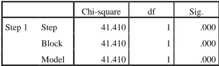
The logistic regression was performed where the independent variable the Probability of Default by the Merton model and dependent variable the failure which can assume the values zero or one.

Table 2. Omnibus Tests of Merton Model Coefficients

Chi-square df Sig. Step 1 Step 41.410 1 .000

Block 41.410 1 .000 Model 41.410 1 .000

22

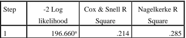
Table 3. Merton Model Summary

Step -2 Log likelihood

Cox & Snell R Square

Nagelkerke R Square 1 196.660a _{.214 .285}

a. Estimation terminated at iteration number 4 because parameter estimates changed by less than .001.

According to Table 4, 74.4% of events were correctly predicted. Furthermore, the model correctly predicted 82.2% of compliant events and 65.9% events of default.

Table 4. Classification Table between Defaulted and Non-defaulted Companies (with Merton model)

Observed Predicted a Default _Percentage Correct 0 1 Step 1 Default 0 74 16 82.2 1 28 54 65.9 Overall Percentage 74.4 a. The cut value is .500

According to Table 5, we find that the Merton variable is statistically significant (using the logit model as regressor) estimator for the probability of default where the independent variable assumes a positive value, indicating that the higher the Merton variable, the higher the probability of default.

Table 5. Variables in the Equation (with Merton model)

B S.E. Wald df Sig. Exp(B) Step 1a _{Merton 3.700 .664 31.096 1 .000 40.451}

Constant -1.017 .227 20.049 1 .000 .362 a. Variable(s) entered on step 1: Merton.

23

5.2 Accounting Model

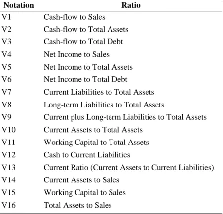
In this chapter we used financial ratios to estimate the probability of default within one year (in the Merton model is used in the same way one year). In Table 6, it is described each variable used in the economic-financial model. These ratios were selected through Beaver (1966).

Table 6. Economic-financial Ratios Used in the Estimation of the Models

Notation Ratio

V1 Cash-flow to Sales V2 Cash-flow to Total Assets V3 Cash-flow to Total Debt V4 Net Income to Sales V5 Net Income to Total Assets V6 Net Income to Total Debt

V7 Current Liabilities to Total Assets V8 Long-term Liabilities to Total Assets

V9 Current plus Long-term Liabilities to Total Assets V10 Current Assets to Total Assets

V11 Working Capital to Total Assets V12 Cash to Current Liabilities

V13 Current Ratio (Current Assets to Current Liabilities) V14 Current Assets to Sales

V15 Working Capital to Sales V16 Total Assets to Sales

Source: Beaver (1966)

In order to perceive the ability to predict failure with economic and financial ratios we used the logit model. Here, we assume the dependent variable as a dummy variable that can take the value zero in case of fulfillment of obligations and one if defaults.

24

Table 7. Omnibus Tests of Accounting Model Coefficients

Chi-square df Sig. Step 1 Step 82.061 14 .000

Block 82.061 14 .000 Model 82.061 14 .000

Table 8. Accounting Model Summary

Step -2 Log likelihood

Cox & Snell R Square

Nagelkerke R Square 1 150.741ª .386 .515 a. Estimation terminated at iteration number 8 because parameter estimates changed by less than .001.

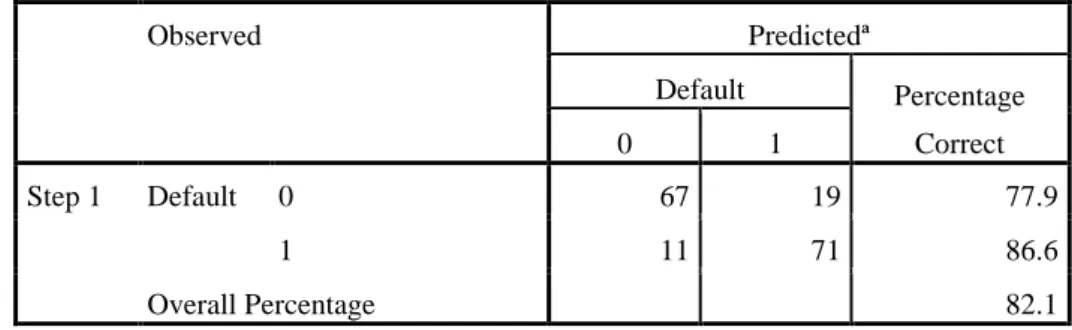
Through Table 9 we find that using financial ratios as estimators of the failure we successfully predicted 82.1% of credit events. Compared to Merton, this model was slightly more robust. Unlike Merton, who successfully predicted 82.2% of compliant events and 65.9% of non-compliant, the use of financial ratios predicted 77.9% and 86.6%, respectively.

Table 9. Classification Table between Defaulted and Non-defaulted Companies (with Economic Financial Ratios)

Observed Predictedª Default _Percentage Correct 0 1 Step 1 Default 0 67 19 77.9 1 11 71 86.6 Overall Percentage 82.1 a. The cut value is .500

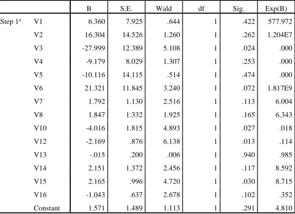
In Table 10 we find that not all accounting variables are significant for the logistic regression model. In fact, only the V3, V10, V12 and V15 variables are statistically significant for a 5% significance level. Notwithstanding, we could not say that V6 is not rejected with a p-value of 0.072, because is very close to 0.05.

25

On an economic basis, the variable V3 behaves as expected, i.e., a decrease of this variable represents an increase in the probability of default. The V10 and V12 variables follow the same rational and present a contrary view regarding the probability of default. On the other hand, variable V15 presents a contrary relationship with the expected. An increase in this variable would generate a decrease in the probability of default. All the other variables in the logit model are not significant.

Table 10. Variables in the Equation (with Economic Financial Ratios)

B S.E. Wald df Sig. Exp(B) Step 1a _{V1 6.360 7.925 .644 1 .422 577.972} V2 16.304 14.526 1.260 1 .262 1.204E7 V3 -27.999 12.389 5.108 1 .024 .000 V4 -9.179 8.029 1.307 1 .253 .000 V5 -10.116 14.115 .514 1 .474 .000 V6 21.321 11.845 3.240 1 .072 1.817E9 V7 1.792 1.130 2.516 1 .113 6.004 V8 1.847 1.332 1.925 1 .165 6.343 V10 -4.016 1.815 4.893 1 .027 .018 V12 -2.169 .876 6.138 1 .013 .114 V13 -.015 .200 .006 1 .940 .985 V14 2.151 1.372 2.456 1 .117 8.592 V15 2.165 .996 4.720 1 .030 8.715 V16 -1.043 .637 2.678 1 .102 .352 Constant 1.571 1.489 1.113 1 .291 4.810 a. Variable(s) entered on step 1: V1, V2, V3, V4, V5, V6, V7, V8, V10, V12, V13, V14, V15, V16.

5.3 Hybrid Model

The Hybrid model includes the estimates of probability of default of the Merton model and the economic-financial ratios in a logit regression.

26

Table 11. Omnibus Tests of Hybrid Model Coefficients

Chi-square df Sig. Step 1 Step 99.712 15 .000

Block 99.712 15 .000 Model 99.712 15 .000

Table 12. Hybrid Model Summary

Step -2 Log likelihood

Cox & Snell R Square

Nagelkerke R Square 1 133.090ª .448 .597 a. Estimation terminated at iteration number 8 because parameter estimates changed by less than .001.

As we can see in Table 13, and as was initially expected, the prediction of the percentage of events, 83.3%, was higher compared to each model used separately. The Hybrid model predicted correctly 86.0% of non-defaulted companies and 80.5% of defaulted companies.

Table 13. Classification Table between Defaulted and Non-defaulted Companies (with Hybrid Model)

Observed Predicted a Default _Percentage Correct 0 1 Step 1 Default 0 74 12 86.0 1 16 66 80.5 Overall Percentage 83.3 a. The cut value is .500

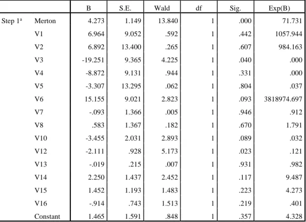
According to Table 14 we find some consistency with previous models, i.e. the Merton variable remains statistically significant with a positive contribution to an increasing risk of default.

Similarly, the V3 and V12 variables remained significant in the model adopting the same relationship to the increase or decrease of risk of default.

27

In contrast, the variables V10 and V15 failed to contribute to the prediction of good and bad companies. Here V6 has a p-value of .093 and V10 has one of .089, and was not rejected at a 10% significance level.

Note also that the significance of all other variables remained the same in the model, i.e., they are not statistically significant.

Table 14. Variables in the Equation (with Hybrid Model)

B S.E. Wald df Sig. Exp(B) Step 1a _{Merton 4.273 1.149 13.840 1 .000 71.731} V1 6.964 9.052 .592 1 .442 1057.944 V2 6.892 13.400 .265 1 .607 984.163 V3 -19.251 9.365 4.225 1 .040 .000 V4 -8.872 9.131 .944 1 .331 .000 V5 -3.307 13.295 .062 1 .804 .037 V6 15.155 9.021 2.823 1 .093 3818974.697 V7 -.093 1.366 .005 1 .946 .912 V8 .583 1.367 .182 1 .670 1.791 V10 -3.455 2.031 2.893 1 .089 .032 V12 -2.111 .928 5.173 1 .023 .121 V13 -.019 .215 .007 1 .931 .982 V14 2.250 1.437 2.452 1 .117 9.487 V15 1.452 1.193 1.483 1 .223 4.273 V16 -.914 .743 1.513 1 .219 .401 Constant 1.465 1.591 .848 1 .357 4.328 a. Variable(s) entered on step 1: Merton, V1, V2, V3, V4, V5, V6, V7, V8, V10, V12, V13, V14, V15, V16.

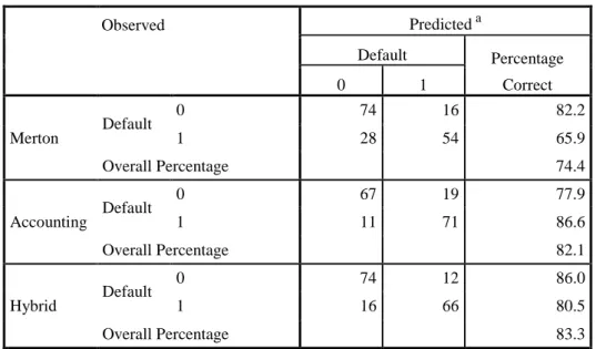
In order to better compare the models, Table 15 shows a summary of the results of the three models applied in this study, the Merton model, Accounting model and Hybrid model. The latter was the one that had a better overall performance and better predictive accuracy on the non-defaulted events. Notwithstanding, the accounting model was the one with a better predictive performance on the defaulted events.

28

Table 15. Summary of Models’ Predictive Accuracy

Observed Predicted a Default _Percentage Correct 0 1 Merton Default 0 74 16 82.2 1 28 54 65.9 Overall Percentage 74.4 Accounting Default 0 67 19 77.9 1 11 71 86.6 Overall Percentage 82.1 Hybrid Default 0 74 12 86.0 1 16 66 80.5 Overall Percentage 83.3 a. The cut value is .500

In Tudela and Young (2003), the Hybrid model predicted 77.09% of events of credit while the structural approach predicted 76.75% and the Accounting model predicted 42.37%. In the same way, in Benos and Papanastasopoulos (2007) the Hybrid model was the one that had a better performance in the classification of credit events, comparing with a Merton approach and an Accounting model. This study is therefore in line with this literature.

29

6. Conclusions, Limitations and Future Research

In this study we analyzed some forecasting techniques of credit failure to listed companies, namely the Merton model, an Accounting model using financial ratios and a Hybrid model that incorporates the two methodologies. The information used was collected in the Moody's URD database and Bloomberg. This study suggests that the Hybrid model confers greater ability to prediction of default comparing with the use of Merton's model and Accounting in a separate way. This is consistent with Tudela and Young (2003).

It should be noticed in this study the limitations concerning the database of companies analyzed. Regarding the number of companies, for future research it is suggested a more extensive companies’ database to calculate the probability of default, thus increasing the robustness of the study. More, due to lack of available data it was considered the period between 1989 and 2010 for defaulted companies and 2012 for non-defaulted. Ideally, it should have been chosen a sample of companies within a smaller period of time, providing a further uniform economic climate. On the other hand, using a single companies’ sector could bring more accurate results to this study.

Also it is noteworthy that the Merton model used also has several limitations in its assumptions, so it would be interesting for future research, for the same study base to apply a model that, for example, allows the default before maturity.

We can thus conclude that the Merton model, despite showing some unrealistic assumptions, gave power to the failure prediction in this study.

30

7. Appendix

Table 16. List of Companies Used in the Study (Cont.)

Company Net Sales Defaulted? Sector Default Date Acme United Corp. $ 84,370.00 No Consumer Products n.d. Blyth Inc. $ 1,179,514.00 No Consumer Products n.d. Capstone Cos Inc. $ 8,363.00 No Consumer Products n.d. Central Garden and Pet Co. $ 1,700,013.00 No Consumer Products n.d. Clorox Co/The $ 5,468,000.00 No Consumer Products n.d. CSS Industries Inc. $ 384,663.00 No Consumer Products n.d. Helen of Troy Ltd. $ 1,181,676.00 No Consumer Products n.d. Jarden Corp. $ 6,696,100.00 No Consumer Products n.d. Kid Brands Inc. $ 229,486.00 No Consumer Products n.d. Kimberly-Clark Corp. $ 21,063,000.00 No Consumer Products n.d. Scott's Liquid Gold-Inc. $ 16,041.00 No Consumer Products n.d. Scotts Miracle-Gro Co/The $ 2,826,100.00 No Consumer Products n.d. Spectrum Brands Holdings Inc. $ 3,252,435.00 No Consumer Products n.d. Summer Infant Inc. $ 247,227.00 No Consumer Products n.d. Tupperware Brands Corp. $ 2,583,800.00 No Consumer Products n.d. WD 40 Co $ 342,784.00 No Consumer Products n.d. Eddie Bauer $ 1,023,437.00 Yes Consumer Products 17-06-2009 Lenox Group, Inc. $ 452,115.00 Yes Consumer Products 23-11-2008 Circuit City Stores, Inc. $ 12,429,800.00 Yes Consumer Products 10-11-2008 Hancock Fabrics, Inc $ 376,179.00 Yes Consumer Products 21-03-2007 Oneida Ltd. $ 350,819.00 Yes Consumer Products 09-03-2006 Salton Inc. $ 1,076,735.00 Yes Consumer Products 26-08-2005 Tropical Sportswear International Inc. $ 386,723.00 Yes Consumer Products 16-12-2004 Huffy Corp. $ 437,676.00 Yes Consumer Products 20-10-2004 Interstate Bakeries Corp. $ 3,525,780.00 Yes Consumer Products 22-09-2004 Dan River Inc. $ 477,448.00 Yes Consumer Products 31-03-2004 Fibermark Inc. $ 397,411.00 Yes Consumer Products 31-03-2004 Cone Mills Corp. $ 445,600.00 Yes Consumer Products 24-09-2003 Guilford Mills, Inc. $ 643,519.00 Yes Consumer Products 13-03-2002 Galey & Lord Inc. $ 849,993.00 Yes Consumer Products 19-02-2002 Kasper A.S.L. $ 383,861.00 Yes Consumer Products 05-02-2002 Vlasic Foods International Inc. $ 901,564.00 Yes Consumer Products 29-01-2001 Converse Inc. $ 209,050.00 Yes Consumer Products 21-01-2001 Pillowtex Corp. $ 1,552,068.00 Yes Consumer Products 14-11-2000 Fruit of the Loom, Inc. $ 1,549,800.00 Yes Consumer Products 29-12-1999

31

Table 16. List of Companies Used in the Study (Cont.)

Company Net Sales Defaulted? Sector Default Date Town & Country Corp. $ 250,578.00 Yes Consumer Products 17-11-1997 Crystal Brands, Inc. $ 444,302.00 Yes Consumer Products 21-01-1994 Clabir Corp. $ 179,359.00 Yes Consumer Products 01-02-1989 ADDvantage Technologies Group Inc. $ 35,216.00 No Distribution n.d. Arrow Electronics Inc. $ 20,405,128.00 No Distribution n.d. Beacon Roofing Supply Inc. $ 2,043,658.00 No Distribution n.d. BlueLinx Holdings Inc. $ 1,907,842.00 No Distribution n.d. Core-Mark Holding Co Inc. $ 8,892,400.00 No Distribution n.d. Educational Development Corp. $ 26,273.00 No Distribution n.d. EnviroStar Inc. $ 22,457.00 No Distribution n.d. Fastenal Co. $ 3,133,577.00 No Distribution n.d. First Aviation Services Inc. $ 21,579.00 No Distribution n.d. Fossil Group Inc. $ 2,857,508.00 No Distribution n.d. Genuine Parts Co. $ 13,013,868.00 No Distribution n.d. Houston Wire & Cable Co. $ 393,036.00 No Distribution n.d. Huttig Building Products Inc. $ 520,500.00 No Distribution n.d. Infosonics Corp. $ 34,294.00 No Distribution n.d. Ingram Micro Inc. $ 37,827,299.00 No Distribution n.d. LKQ Corp. $ 4,122,930.00 No Distribution n.d. MWI Veterinary Supply Inc. $ 2,075,146.00 No Distribution n.d. Owens & Minor Inc. $ 8,908,145.00 No Distribution n.d. Pool Corp. $ 1,953,974.00 No Distribution n.d. Precision Aerospace Components Inc. $ 20,240.00 No Distribution n.d. ScanSource Inc. $ 3,015,296.00 No Distribution n.d. SED International Holdings Inc. $ 577,274.00 No Distribution n.d. Speed Commerce Inc. $ 480,824.00 No Distribution n.d. Titan Machinery Inc. $ 2,198,420.00 No Distribution n.d. United Stationers Inc. $ 5,080,106.00 No Distribution n.d. Vapor Corp. $ 21,353.00 No Distribution n.d. WESCO International Inc. $ 6,579,301.00 No Distribution n.d. WW Grainger Inc. $ 8,950,045.00 No Distribution n.d. FAO Inc. $ 460,415.00 Yes Distribution 04-12-2003 Samuels Jewelers, Inc. $ 122,007.00 Yes Distribution 04-08-2003 Daisytek International Inc. $ 1,185,030.00 Yes Distribution 03-06-2003 Pentacon Inc. $ 259,351.00 Yes Distribution 23-05-2002 Dairy Mart Convenience Stores $ 723,671.00 Yes Distribution 24-09-2001 Phar-Mor Inc. $ 1,292,090.00 Yes Distribution 21-09-2001

32

Table 16. List of Companies Used in the Study (Cont.)

Company Net Sales Defaulted? Sector Default Date Homeland Holding Corp. $ 600,835.00 Yes Distribution 01-08-2001 Zany Brainy, Inc. $ 400,479.00 Yes Distribution 15-05-2001 US Office Products Company $ 2,499,393.00 Yes Distribution 05-03-2001 Waxman Industries Inc. $ 99,116.00 Yes Distribution 02-10-2000 Heilig-Meyers Corp $ 2,726,358.00 Yes Distribution 16-08-2000 Trend-Lines Inc. $ 262,550.00 Yes Distribution 11-08-2000 Flooring America Inc. $ 762,808.00 Yes Distribution 15-06-2000 Eagle Food Centers Inc. $ 932,789.00 Yes Distribution 29-02-2000 AgriBioTech Inc. $ 370,453.00 Yes Distribution 26-01-2000 Just for Feet Inc. $ 776,162.00 Yes Distribution 04-11-1999 Service Merchandise Company $ 3,159,260.00 Yes Distribution 27-03-1999 Levitz Furniture Incorporated $ 986,622.00 Yes Distribution 05-09-1997 Barry's Jewelers Inc. $ 140,145.00 Yes Distribution 12-05-1997 Fretter Inc. $ 502,317.00 Yes Distribution 24-09-1996 Caldor Corp. $ 2,748,634.00 Yes Distribution 18-09-1995 House of Fabrics, Inc. $ 546,664.00 Yes Distribution 02-11-1994 National Convenience Stores Inc. $ 1,062,183.00 Yes Distribution 09-12-1991 S.E. Nichols, Inc. $ 214,315.00 Yes Distribution 02-08-1990 Circle K Corp. $ 3,493,107.00 Yes Distribution 15-05-1990 Advanced Medical Isotope Corp. $ 248.00 No Manufacturing n.d. American Railcar Industries Inc. $ 711,723.00 No Manufacturing n.d. AptarGroup Inc. $ 2,331,036.00 No Manufacturing n.d. Cyclone Power Technologies Inc. $ 1,134.00 No Manufacturing n.d. FreightCar America Inc. $ 677,449.00 No Manufacturing n.d. Hillenbrand Inc. $ 983,200.00 No Manufacturing n.d. John Bean Technologies Corp. $ 917,300.00 No Manufacturing n.d. LGA Holdings Inc. $ 515.00 No Manufacturing n.d. Movado Group Inc. $ 505,478.00 No Manufacturing n.d. Organic Plant Health Inc. $ 873.00 No Manufacturing n.d. Ourpet's Co. $ 20,161.00 No Manufacturing n.d. Powin Corp. $ 42,306.00 No Manufacturing n.d. Spire Corp. $ 22,110.00 No Manufacturing n.d. TriMas Corp. $ 1,272,910.00 No Manufacturing n.d. Builders FirstSource, Inc. $ 677,886.00 Yes Manufacturing 22-01-2010 Champion Enterprises, Inc. $ 1,033,193.00 Yes Manufacturing 15-11-2009 Building Materials Holding Corporation $ 1,324,679.00 Yes Manufacturing 16-06-2009 Foamex International Inc. $ 1,266,394.00 Yes Manufacturing 15-09-2005

33

Table 16. List of Companies Used in the Study (Cont.)

Company Net Sales Defaulted? Sector Default Date DT Industries Inc. $ 241,066.00 Yes Manufacturing 13-05-2004 Reunion Industries Inc. $ 70,799.00 Yes Manufacturing 03-12-2003 Oakwood Homes Corp. $ 1,133,445.00 Yes Manufacturing 15-11-2002 ACT Manufacturing Inc. $ 1,370,597.00 Yes Manufacturing 21-12-2001 Tokheim Corporation $ 693,932.00 Yes Manufacturing 28-08-2000 Trikon Technologies Inc. $ 85,109.00 Yes Manufacturing 14-05-1998 Cooper Companies, Inc. $ 92,652.00 Yes Manufacturing 06-01-1994 Emerson Radio Corp. $ 764,152.00 Yes Manufacturing 29-09-1993 Intermark Inc. $ 400,845.00 Yes Manufacturing 19-10-1992 Sudbury Inc. $ 376,182.00 Yes Manufacturing 10-01-1992 Eagle-Picher Industries Inc. $ 699,347.00 Yes Manufacturing 07-01-1991 Amdura Corp. $ 156,715.00 Yes Manufacturing 02-04-1990 Amdocs Ltd. $ 190,875.00 No Telecommunications n.d. Aviat Networks Inc. $ 444,000.00 No Telecommunications n.d. Consolidated Communications Holdings Inc. $ 503,457.00 No Telecommunications n.d. CPS Technologies Corp. $ 14,052.00 No Telecommunications n.d. CTI Group Holdings Inc. $ 16,759.00 No Telecommunications n.d. Digerati Technologies Inc. $ 4,135.00 No Telecommunications n.d. EarthLink Holdings Corp. $ 1,348,977.00 No Telecommunications n.d. Elephant Talk Communications Corp. $ 29,202.00 No Telecommunications n.d. FairPoint Communications Inc. $ 973,649.00 No Telecommunications n.d. Fusion Telecommunications International Inc. $ 44,288.00 No Telecommunications n.d. Global Mobiletech Inc. $ 15,402.00 No Telecommunications n.d. Glowpoint Inc. $ 29,070.00 No Telecommunications n.d. GTT Communications Inc. $ 107,877.00 No Telecommunications n.d. Hawaiian Telcom Holdco Inc. $ 385,498.00 No Telecommunications n.d. HC2 Holdings Inc. $ 260,554.00 No Telecommunications n.d. ICTC Group Inc. $ 4,078.00 No Telecommunications n.d. Inteliquent Inc. $ 275,453.00 No Telecommunications n.d. Level 3 Communications Inc. $ 6,376,000.00 No Telecommunications n.d. Lightyear Network Solutions Inc. $ 66,441.00 No Telecommunications n.d. Lumos Networks Corp. $ 206,871.00 No Telecommunications n.d. LYFE Communications Inc. $ 532.00 No Telecommunications n.d. MDU Communications International Inc. $ 27,305.00 No Telecommunications n.d. Net Talk.com Inc. $ 5,791.00 No Telecommunications n.d. NeuStar Inc. $ 831,388.00 No Telecommunications n.d. New ULM Telecom Inc. $ 32,483.00 No Telecommunications n.d.

34

Table 16. List of Companies Used in the Study (Cont.)

Company Net Sales Defaulted? Sector Default Date ORBCOMM Inc. $ 64,498.00 No Telecommunications n.d. Premiere Global Services Inc. $ 504,960.00 No Telecommunications n.d. RigNet Inc. $ 161,669.00 No Telecommunications n.d. Single Touch Systems Inc. $ 6,347.00 No Telecommunications n.d. Telkonet Inc. $ 12,758.00 No Telecommunications n.d. TW Telecom Inc. $ 1,470,255.00 No Telecommunications n.d. USA Mobility Inc. $ 219,696.00 No Telecommunications n.d. Suncom Wireless Holdings Inc. $ 852,879.00 Yes Telecommunications 31-01-2007 Choice One Communications Inc. $ 322,891.00 Yes Telecommunications 05-10-2004 Alamosa Holdings Inc. $ 555,692.00 Yes Telecommunications 11-11-2003 Allegiance Telecom Inc. $ 770,982.00 Yes Telecommunications 14-05-2003 NTELOS Inc. $ 261,627.00 Yes Telecommunications 04-03-2003 Qwest Communications International Inc. $ 19,695,000.00 Yes Telecommunications 26-12-2002 Focal Communications Corp. $ 317,485.00 Yes Telecommunications 19-12-2002 CTC Communications Group Inc. $ 299,438.00 Yes Telecommunications 03-10-2002 ITC Deltacom Inc. $ 415,339.00 Yes Telecommunications 25-06-2002 Neon Communications Inc. $ 26,551.00 Yes Telecommunications 25-06-2002 NTL Inc. $ 3,699,200.00 Yes Telecommunications 08-05-2002 Talk America Holdings $ 495,470.00 Yes Telecommunications 01-04-2002 Covad Communications Group Inc. $ 158,736.00 Yes Telecommunications 15-08-2001 Weblink Wireless Inc. $ 289,976.00 Yes Telecommunications 23-05-2001 Teligent Inc. $ 152,072.00 Yes Telecommunications 21-05-2001 Viatel Inc. $ 749,453.00 Yes Telecommunications 02-05-2001 GST Telecommunications Inc. $ 321,922.00 Yes Telecommunications 17-05-2000 Wireless One Inc. $ 38,737.00 Yes Telecommunications 10-02-1999 Geotek Communications, Inc. $ 65,510.00 Yes Telecommunications 29-06-1998

35

8. References

Altman, E. I. (1968). Financial Ratios, Discriminant Analysis and the Prediction of Corporate Bankruptcy. The Journal of Finance, Volume 23, 589–734.

Altman, E. I. (2000). Predicting Financial Distress Of Companies: Revisiting The Z-Score And Zeta. Obtido de NYU Stern: http://pages.stern.nyu.edu/~ealtman/PredFnclDistr.pdf

Arora, N., Bohn, J. R., & Zhu, F. (2005). Reduced Form vs. Structural Models of Credit Risk: A Case Study of Three Models. Journal of Investment Management, Vol. 3, No. 4.

Beaver, W. H. (1966). Financial Ratios as Predictors of Failure. Journal of Accounting Research, Vol. 4, Supplement, 71-111.

Benos, A., & Papanastasopoulos, G. (2007). Extending the Merton Model: A Hybrid Approach to Assessing Credit Quality. 47-68: Mathematical and Computer Modeling, Vol. 46.

Bharath, S. T., & Shumway, T. (2008). Forecasting Default with the Merton Distance to Default Model. Review of Financial Studies 21, 1339-1369.

Black, F., & Scholes, M. (1973). The Pricing of Options and Corporate Liabilities. The Journal of Political Economy, Vol. 81, No. 3, 637-654.

Bohn, J., Arora, N., & Korablev, I. (2005a). Power and Level Validation of the EDF™ Credit Measure in the U.S. Moody's KMV.

Cossin, D., & Pirotte, H. (2001). Advanced Credit Risk Analysis: Financial Approaches and Mathematical Models to Assess, Price, and Manage Credit Risk. New York: Wiley and Sons.

Crosbie, P., & Bohn, J. (2003). Modeling Default Risk. KMV LLC.

Duffie, D., & Singleton, K. J. (1999). Modeling Term Structures of Defaultable Bonds. Review of Financial Studies, 12, 687-720.