Universidade do Minho
Escola de Engenharia Departamento de Inform´atica
Raquel Sim˜oes
Distinguishing kinships beyond identity and paternity
Universidade do Minho
Escola de Engenharia Departamento de Inform´atica
Raquel Sim˜oes
Distinguishing kinships beyond identity and paternity
Master dissertation
Master Degree in Bioinformatics
Dissertation supervised by
Eduardo Conde-Sousa N ´adia Pinto
A C K N O W L E D G E M E N T S
First and foremost, I have to thank my research supervisors, Eduardo Conde-Sousa and N´adia Pinto. Without their assistance and dedicated involvement in every step throughout the process, this paper would have never been accomplished. I would like to thank you very much for your support and understanding over this important stage of my life.
In September 2015, I went to the University of Minho for two years of study and this time has been highly productive and enriching. I was initially very doubtful if I should really follow this path, but today, if I went back I would do exactly the same thing again.
Getting through my dissertation required more than academic support, and I have many, many people to thank for listening to and, at times, having to tolerate me over this time. Most importantly, none of this could have happened without my family and closest friends. Thank you to all!
A B S T R A C T
In kinship testing powerful statistical results are usually obtained when genetic infor-mation is expected to be shared between a pair of samples, which happens in paternity and identification testing. However, there are other pedigrees where genetic information shar-ing is not required, such as when a pair of full-siblshar-ings or avuncular, is analyzed. Studyshar-ing these pedigrees, where the sharing of genetic information is not mandatory, will be the focus of this work. We will consider several kinship problems where two (exhaustive and mutually exclusive) hypotheses will be compared, through a statistical evaluation based on the calculation of a likelihood ratio (LR) where the probabilities of genotypic configurations, assuming one or another kinship hypothesis, are compared. This analysis will allow the identification of the proportion of cases where the statistical evaluation had weak results, and those where LR favored the false hypothesis of kinship for a widely used commercial kit of genetic markers, considering simulated profiles assuming the pedigrees in question. In addition, we will compare the statistical gain of increasing the battery of analyzed mark-ers and infer the impact of considering the genetic information given by the knowledge of the genetic profile of a relative, as the undoubted mother in the case where the hypothe-ses ”individuals A and B are related as full-siblings“ and ”the individuals A and B are unrelated“ are asked to be compared. Furthermore, a validation of the Familias software for two individuals will be performed for the simplest assumptions - absence of mutation and absence of silent allele - through the implementation of the algebraic formulas already established.
R E S U M O
Em testes de parentesco, resultados estat´ısticos poderosos s˜ao geralmente obtidos quando a partilha de informac¸˜ao gen´etica ´e esperada entre um par de amostras, o que acontece em testes de paternidade e de identificac¸˜ao. No entanto, existem outros pedigrees onde a partilha de informac¸˜ao gen´etica n˜ao ´e requerida, como quando um par de irm˜aos ou tia(o)/sobrinha(o) ´e analisado. Estudar estes pedigrees, onde a partilha de informac¸˜ao gen´etica n˜ao ´e obrigat ´oria, ser´a o foco deste trabalho. Consideraremos v´arios problemas de parentesco em que duas hip ´oteses (exaustivas e mutuamente exclusivas) ser˜ao compara-das, atrav´es de uma avaliac¸˜ao estat´ıstica com base no c´alculo de raz ˜oes de verossimilhanc¸a (LR, do inglˆes likelihood ratio) onde as probabilidades das configurac¸ ˜oes genot´ıpicas, as-sumindo uma ou outra hip ´otese de parentesco, s˜ao comparadas. Esta an´alise permitir´a a identificac¸˜ao da proporc¸˜ao de casos em que a avaliac¸˜ao estat´ıstica teve resultados fracos, e aqueles onde o LR favoreceu a hip ´otese falsa de parentesco para um kit comercial am-plamente utilizado de marcadores gen´eticos, considerando perfis simulados assumindo os pedigrees em quest˜ao. Adicionalmente, ser´a comparado o ganho estat´ıstico de aumentar a bateria dos marcadores analisados e ser´a tamb´em inferido o impacto de considerar a informac¸˜ao gen´etica dada pelo conhecimento do perfil gen´etico de um parente, como a m˜ae indubitada no caso em que as hip ´oteses ”indiv´ıduos A e B est˜ao relacionadas como irm˜aos“ e ”os indiv´ıduos A e B n˜ao est˜ao relacionados” s˜ao comparadas. Al´em disso, uma validac¸˜ao do software Familias para dois indiv´ıduos ser´a realizada para os pressu-postos mais simples - ausˆencia de mutac¸˜ao e inexistˆencia de alelo silencioso - atrav´es da implementac¸˜ao de f ´ormulas alg´ebricas j´a estabelecidas.
C O N T E N T S
1 i n t r o d u c t i o n 2
1.1 Context and Motivation 2
1.2 Genetic inheritance 4
1.3 Genetic Markers 9
1.4 Mutation Models 10
1.4.1 The equal model 10
1.4.2 The proportional model 11
1.4.3 The stepwise model 11
1.4.4 The extended stepwise model 12
1.4.5 An example illustrating how use the mutation models 12
1.5 Statistical Evaluation 15
1.5.1 Hypotheses 15
1.5.2 Likelihood Ratio 16
1.5.3 Identity-by-descent versus identity-by-state 17
2 s tat e o f t h e a r t 19
2.1 Exact Algebraic Expressions 19
2.2 Software 21 2.3 Software Validation 22 3 o b j e c t i v e s 24 4 m at e r i a l a n d m e t h o d s 25 4.1 Kinship problems 25 4.2 Database 26
4.3 Simulation of genetic profiles 27
4.4 Validation of Familias for the simplest assumptions - absence of mutation
and presence of silent allele 28
4.5 Measurement of the impact of considering a third individual and/or a greater
number of markers 28
5 r e s u lt s 30
5.1 Validation of Familias for the simplest assumptions - absence of mutation
and silent allele 30
5.2 Measurement of the impact of considering a third individual and/or a greater
number of markers 31
5.2.1 Full-Siblings versus Half-Siblings 31
Contents v
5.2.2 Full-Siblings versus Unrelated 37
5.2.3 Half-Siblings versus Unrelated 42
5.2.4 Avuncular versus Unrelated 48
5.2.5 First Cousins versus Unrelated 53
5.2.6 Half First Cousins versus Unrelated 58
6 c o n c l u s i o n s 63
6.1 Validation of Familias for the simplest assumptions - absence of mutation
and silent allele 63
6.2 Measurement of the impact of considering a third individual and/or a greater
number of markers 63
L I S T O F F I G U R E S
Figure 1 The seven traits observed by Mendel in pea plants, from Nature
Ed-ucation Adapted from Pierce (2013). 4
Figure 2 Mendel’s monohybrid crosses, from Nature Education Adapted from
Pierce (2013). 5
Figure 3 Mendel’s dihybrid cross, from Nature Education Adapted from Pierce
(2013). 6
Figure 4 Examples of uniparental and biparental pedigrees. 20
Figure 5 Representation of the six cases under study. 26
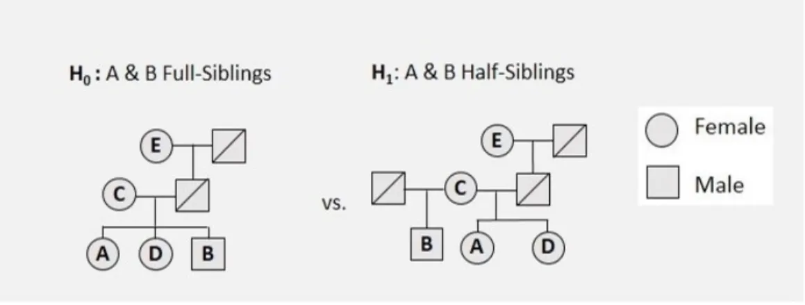
Figure 6 Representation of the hypotheses H0: ”A and B are related as
full-siblings“ and H1:”A and B are related as half-siblings“ - Figure 5(a.). 31
Figure 7 Distribution of LR= P(G|FS)
P(G|HS) values (10-log scale, results for A and B
simulated as FS and HS in full line and dashed line, respectively) ob-tained when considering the hypotheses depicted at Figure 5 (a.) and assuming sets of analyzed individuals: {A,B} (blue line), {A,B,C} (orange line), {A,B,D} (dark red line) and {A,B,E} (green line) for 17
autosomal markers. x-axis: log10(LR); y-axis: density. 32
Figure 8 Distribution of LR = P(G|FS)
P(G|HS) values (10-log scale, results for A and
B simulated as FS and HS in full line and dashed line, respectively) obtained when considering the hypotheses depicted at Figure 5 (a.) and assuming sets of analyzed individuals: {A,B} (blue line) for 35 autosomal markers and {A,B,D} (orange line) for 17 autosomal
markers. x-axis: log10(LR); y-axis: density. 33
Figure 9 Distribution of LR= P(G|FS)
P(G|HS) values (10-log scale, results for A and B
simulated as FS and HS in full line and dashed line, respectively) ob-tained when considering the hypotheses depicted at Figure 5 (a.) and assuming sets of analyzed individuals: {A,B} (blue line), {A,B,C} (orange line), {A,B,D} (dark red line) and {A,B,E} (green line), for
different numbers of markers: 17, 22, 27, 32 and 35. x-axis: log10(LR);
y-axis: density. Data summarized in Table 6. 35
Figure 10 Representation of the hypotheses H0: ”A and B are related as
full-siblings“ and H1:”A and B are unrelated“ - Figure 5(b.). 37
List of Figures vii
Figure 11 Distribution of LR= PP((GG||UnrFS)) values (10-log scale, results for A and
B simulated as FS and Unr in full line and dashed line, respec-tively) obtained when considering the hypotheses depicted at Figure
5(b.) and assuming sets of analyzed individuals: {A,B} (blue line),
{A,B,C} (orange line), {A,B,D} (dark red line) and {A,B,E} (green
line) for 17 autosomal markers. x-axis: log10(LR); y-axis: density. 39
Figure 12 Distribution of LR= PP((GG||UnrFS)) values (10-log scale, results for A and
B simulated as FS and Unr in full line and dashed line, respec-tively) obtained when considering the hypotheses depicted at Figure
5(b.) and assuming sets of analyzed individuals: {A,B} (blue line),
{A,B,C} (orange line), {A,B,D} (dark red line) and {A,B,E} (green line), for different numbers of markers: 17, 22, 27, 32 and 35. x-axis:
log10(LR); y-axis: density. Data summarized in Table 7. 40
Figure 13 Representation of the hypotheses H0: ”A and B are related as
half-siblings“ and H1:”A and B are unrelated“ - Figure 5(c.). 42
Figure 14 Distribution of LR= PP((GG||UnrHS)) values (10-log scale, results for A and
B simulated as HS and Unr in full line and dashed line, respectively) obtained when considering the hypotheses depicted at Figure 5 (c.) and and assuming sets of analyzed individuals: {A,B} (blue line) for 35 STRs, {A,B,C} (orange line) for 27 STRs, {A,B,D} (dark red line)
for 22 STRs and {A,B,E} (green line) for 22 STRs. x-axis: log10(LR);
y-axis: density. 43
Figure 15 Distribution of LR= P(G|HS)
P(G|Unr) values (10-log scale, results for A and
B simulated as HS and Unr in full line and dashed line, respectively) obtained when considering the hypotheses depicted at Figure 5 (c.) and assuming sets of analyzed individuals: {A,B} (blue line) for 35 STRs, {A,B,C} (orange line) for 35 STRs, {A,B,D} (dark red line) for
32 STRs and {A,B,E} (green line) for 27 STRs. x-axis: log10(LR);
y-axis: density. 45
Figure 16 Distribution of LR= PP((GG||UnrHS)) values (10-log scale, results for A and
B simulated as HS and Unr in full line and dashed line, respec-tively) obtained when considering the hypotheses depicted at Figure
5 (c.) and assuming sets of analyzed individuals: {A,B} (blue line),
{A,B,C} (orange line), {A,B,D} (dark red line) and {A,B,E} (green line), for different numbers of markers: 17, 22, 27, 32 and 35. x-axis:
log10(LR); y-axis: density. Data summarized in Table 8. 46
Figure 17 Representation of the hypotheses H0: ”A and B are related as
List of Figures viii
Figure 18 Distribution of LR= PP((GG||UnrAV)) values (10-log scale, results for A and
B simulated as AV and Unr in full line and dashed line, respectively) obtained when considering the hypotheses depicted at Figure 5 (d.) and assuming sets of analyzed individuals: {A,B,C} (blue line) for 32 STRs, {A,B,D} (orange line) for 32 STRs and {A,B,E} (dark red
line) for 35 STRs. x-axis: log10(LR); y-axis: density. 50
Figure 19 Distribution of LR= PP((GG||UnrAV)) values (10-log scale, results for A and
B simulated as AV and Unr in full line and dashed line, respec-tively) obtained when considering the hypotheses depicted at Figure
5(d.) and assuming sets of analyzed individuals: {A,B} (blue line),
{A,B,C} (orange line), {A,B,D} (dark red line) and {A,B,E} (green line), for different numbers of markers: 17, 22, 27, 32 and 35. x-axis:
log10(LR); y-axis: density. Data summarized in Table 9. 51
Figure 20 Representation of the hypotheses H0: ”A and B are related as first
cousins“ and H1: ”A and B are unrelated“ - Figure 5(e.). 53
Figure 21 Distribution of LR= PP((GG||UnrFC)) values (10-log scale, results for A and
B simulated as FC and Un in full line and dashed line, respectively) obtained when considering the hypotheses depicted at Figure 5 (e.) and assuming sets of analyzed individuals: {A,B} (blue line) for 35 STRs, {A,B,C} (orange line) for 27 STRs and {A,B,D} (dark red line)
for 17 STRs. x-axis: log10(LR); y-axis: density. 54
Figure 22 Distribution of LR= PP((GG||UnrFC)) values (10-log scale, results for A and
B simulated as FC and Unr in full line and dashed line, respec-tively) obtained when considering the hypotheses depicted at Fig-ure 5 (e.) and assuming sets of analyzed individuals: {A,B} (blue line), {A,B,C} (orange line) and {A,B,D} (dark red line), for different
numbers of markers: 17, 22, 27, 32 and 35. x-axis: log10(LR); y-axis:
density. Data summarized in Table 10. 56
Figure 23 Representation of the hypotheses H0: ”A and B are related as half
first cousins“ and H1: ”A and B are unrelated“ - Figure 5(f.). 58
Figure 24 Distribution of LR= PP((GG||UnrHC)) values (10-log scale, results for A and
B simulated as HC and Un in full line and dashed line, respectively) obtained when considering the hypotheses depicted at Figure 5 (f.) and assuming sets of analyzed individuals: {A,B} (blue line) for 35 STRs, {A,B,C} (orange line) for 35 STRs and {A,B,D} (dark red line)
List of Figures ix
Figure 25 Distribution of LR= PP((GG||UnrHC)) values (10-log scale, results for A and
B simulated as HC and Unr in full line and dashed line, respec-tively) obtained when considering the hypotheses depicted at Fig-ure 5 (f.) and assuming sets of analyzed individuals: {A,B} (blue line), {A,B,C} (orange line) and {A,B,D} (dark red line), for different
numbers of markers: 17, 22, 27, 32 and 35. x-axis: log10(LR); y-axis:
L I S T O F TA B L E S
Table 1 Properties of allele system. 12
Table 1 Identity by descent (IBD) partitions for some pedigrees (adapted
from (Weir et al., 2006)). 18
Table 2 The seven distinct patterns of genotypes that result in seven
alge-braic expressions, that are possible for two non-inbred individuals and codominant alleles at one autosomal locus (adapted from (Weir
et al., 2006)); Pi represents the frequency of the i allele and ksthe s-th
IBD partition associated with the pedigree linking the individuals;
“Hom” being homozygous and “Het” being heterozygous. 19
Table 3 The algebraic expressions for testing some biological relationships
among three individuals (adapted from (Fung et al., 2006)). The joint genotype probabilities P(X,Y,Z), for all possible genetic
config-urations of X, Y, and Z. 21
Table 4 The hypotheses to be compare that derive from Figure 5. 26
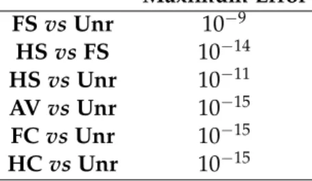
Table 5 Maximum error per cases under study after analyzing 35 STR
sys-tems. 30
Table 6 LRT results obtained for 100 000 simulated families, comparing the
hypotheses of the individuals A and B being related as full-siblings (FS) or as half-siblings (HS) - see Figure 5 (a.)- assuming different sets
of analyzed individuals: {A,B}, {A,B,C}, {A,B,D} and {A,B,E}. 36
Table 7 LRT results obtained for 100 000 simulated families, comparing the
hypotheses of the individuals A and B being related as full-siblings (FS) or as Unrelated (Unr) - see Figure 5 (b.)- assuming different sets
of analyzed individuals: {A,B}, {A,B,C}, {A,B,D} and {A,B,E}. 41
Table 8 LRT results obtained for 100 000 simulated families, comparing the
hypotheses of the individuals A and B being related as half-siblings (HS) or as Unrelated (Unr) - see Figure 5 (b.)- assuming different sets
of analyzed individuals: {A,B}, {A,B,C}, {A,B,D} and {A,B,E}. 47
Table 9 LRT results obtained for 100 000 simulated families, comparing the
hypotheses of the individuals A and B being related as avuncular (AV) or as Unrelated (Unr) - see Figure 5 (d.)- assuming different sets
of analyzed individuals: {A,B}, {A,B,C}, {A,B,D} and {A,B,E}. 52
List of Tables xi
Table 10 LRT results obtained for 100 000 simulated families, comparing the
hypotheses of the individuals A and B being related as first cousins (FC) or as Unrelated (Unr) - see Figure 5 (e.)- assuming different sets
of analyzed individuals: {A,B}, {A,B,C} and {A,B,D}. 57
Table 11 LRT results obtained for 100 000 simulated families, comparing the
hypotheses of the individuals A and B being related as half first cousins (HC) or as Unrelated (Unr) - see Figure 5 (f.)- assuming dif-ferent sets of analyzed individuals: {A,B}, {A,B,C} and {A,B,D}. 62
A C R O N Y M S
Aadenine.
AVavuncular.
Ccytosine.
COTS Commercial off-the-shelf.
DNADeoxyribonucleic acid.
DVIDisaster victim identification.
FCfirst cousins.
FSfull-siblings.
Gguanine.
GHEP-ISFG The Spanish and Portuguese Speaking Working Group of the International Society for Forensic Genetics.
HC half first cousins.
HShalf-siblings.
IBDidentity by descent.
IBSidentity by state.
IMinteger mutations.
LRlikelihood ratio.
MVM microvariant mutations.
RFLPRestriction Fragment Length Polymorphism.
SNPsSingle Nucleotide Polymorphisms.
SSRsSimple Sequence Repeats.
STRShort Tandem Repeat.
Tthymine.
Unrunrelated.
1
I N T R O D U C T I O N
1.1 c o n t e x t a n d m o t i vat i o n
Forensic Genetics is the branch of genetics that makes use of the knowledge and tech-niques of genetics and molecular biology in helping to resolve problems and legal proce-dures (Jobling and Gill, 2004). Thus, the purpose of a forensic geneticist is to evaluate the likelihood of specific genetic kinships between samples and/or individuals, providing un-biased and statistically supported information (Pinto et al., 2009). Forensic Genetics based on Deoxyribonucleic acid (DNA) started in the 1980s when researchers found highly vari-able DNA regions. Nowadays, DNA analysis is an indispensvari-able routine part of modern forensic casework (Jobling and Gill, 2004; Wyman and White, 1980). The sources for the bi-ological evidence used in a forensic context are, for example, any body fluid (such as blood, semen, saliva or urine), bones, teeth, hairs, furs, muscle tissue or even touched objects.
Analyses on Forensic Genetics generally fall into one of the following frameworks:
(a.) analysis of mixtures, generally aiming identification tests, where the sample contains
DNA from two or more contributors. In most cases, experts have to deal with degraded and/or contaminated samples and with a low amount of DNA. For example, the compati-bility between the genetic profile of one suspect and the sample recovered from the crime scene, or in cases of sexual assaults where the material collected has genetic material from the victim and the perpetrator(s). Therefore the main objective is to carry out identification tests;
(b.) kinship analysis, in the majority of the cases aiming paternity tests, where reference
samples (with good quantity/quality of DNA) are used. In criminal context, paternity tests can be computed, for example, when rapes result in pregnancy and only then is denounced/investigated (situations commonly involving intellectually disabled women). Other situations can be related with immigration cases (evaluation of the kinship existing between an individual applying for a visa and a legal immigrant already established in the country) or inheritance claims, where the alleged parent can be available for testing or
1.1. Context and Motivation 3
not. Another example is in identification following disasters - the so-called Disaster victim identification (DVI) problems.
However, (a.) and (b.) can intersect, that is, sometimes it is necessary to compute kinship tests considering samples which are mixtures. An example of this is when there is material of abortion, resulting from a sexual assault, where the profile of the fetus is not distinguish-able from the mother (mixture), even having access to the genetic profile of hers (and of the putative father).
Genealogical and pedigree reconstruction has been a subject of high importance, not only for humans, but also for non-human populations. Applications arise, for example, in studies of inbreeding and conservation of species. Indeed, using genetic information to study relationships among human and non-human individuals is a broad topic with a large number of fields of application.
Note that, unlike other forensic areas that rely on the expert’s analysis on an intuitive ba-sis of expertise, forensic genetics has a formal framework based on probability theory and quantification of the proof. Therefore, it is necessary to have knowledge of the genetic char-acterization of the population by carrying out a quantitative evaluation though population genetics studies. By way of example, if for a specific marker, a suspect has a genetic profile coincident with the one of a sample recovered from a crime scene, the evidence is valued differently if the profile is rare or common in the population. Hence, forensic genetics is a discipline of population genetics.
Within kinship analyses, very powerful statistical results are usually obtained, as the sharing of genetic information is required - in identity (or monozygosity twins) and parent-child analyses. However, there are other pedigrees where the sharing of genetic information is not required as, for example, in case of full(or half)-siblings or avuncular.
Throughout this thesis a study will be performed based on inferring genealogical rela-tionships among those pedigrees, where the sharing of genetic information is not manda-tory. Different sets of independent markers routinely used in many laboratories worldwide will be considered for the statistical analyses. The gain of increasing the battery of analyzed autosomal markers and the impact of adding an extra relative (for example, the undoubted mother), will be studied. This analysis will give us guidance on which relatives should be chosen from an initial set of candidates and the number of markers needed to be ana-lyzed in order to maximize the chance of achieving a statistic powerful result. Moreover, we will perform a validation of the software Familias, widely used by forensic laboratories worldwide to compute likelihoods in relationship scenarios.
1.2. Genetic inheritance 4
1.2 g e n e t i c i n h e r i ta n c e
Gregor Mendel (1822 − 1884), through his work on pea plants, discovered the
funda-mental laws of inheritance in 1865 and, because of that, he is known as the father of genetics. Our modern understanding of how traits may be inherited through generations comes from the principles proposed by this monk ((Mendel, 1866), for the English translation: (Mendel,
1901)). See box below for an overview on Mendel’s experience.
Mendel picked common garden pea plants (of the species Pisum sativum) for the focus of his research because they can be grown easily in large numbers, have distinct contrasting traits (for example, the color of the seed is either green or yellow) and their reproduction can be manipulated. Pea plants have both male and female reproductive organs. As a result, they can either self-pollinate (pollen could come from the same flower) or cross-self-pollinate with another plant (pollen could come from another plant’s flowers). So, he could easily control their fertilization by transferring pollen with a small paintbrush.
In his experiments, Mendel observed seven different characteristics in the pea plants, and each of these characteristics had two contrasting forms (see Figure 1). The characteristics included, for example, height (tall or short), pod shape (inflated or constricted), seed shape (smooth or winkled) or pea color (green or yellow).
Figure 1: The seven traits observed by Mendel in pea plants, from Nature Education Adapted from Pierce (2013).
In the first stage, Mendel wanted to obtain pure lineages for the selected characteristics in order to initialize his study. Once the characteristics of the pea plant were consistent generation after generation of self-fertilization (for
1.2. Genetic inheritance 5
example, green plants had only green children and grandchildren and so forth), these parental lines of peas were considered pure-breeders.
When conducting his experiments, Mendel designated the two pure-breeding parental generations involved in a particular cross as P, and the off-spring resulting from the crossing of P as F1 generation. Here, Mendel noticed that the F1 generation looked like one parent of the P generation. Upon ob-serving the uniformity of the F1 generation, Mendel wondered whether the F1 generation could still possess the non-dominant traits of the other parent in some hidden way. To understand whether traits were hidden in the F1 gener-ation, Mendel returned to the method of self-fertilization. Here, he created an F2 generation by letting an F1 pea plant self-fertilize.
Figure 2: Mendel’s monohybrid crosses, from Nature Education Adapted from Pierce (2013).
As Mendel suspected, the two traits are observable in the resulting F2 gen-eration. Also, when he averaged the relative proportion of both characteristics across all F2 progeny sets, he found that one trait was consistently three times more frequent than the other (3:1). Figure 2 shows an example of Mendel’s data for the seed form (round or wrinkled), but note that Mendel studied all seven cases and in all he obtained the same conclusions. Thus, the Law of Segregation emerges, also known as Mendels’ first law, stating that every in-dividual organism contains two “particle” for each trait and to a specific trait each “particle” came from each parent.
1.2. Genetic inheritance 6
Mendel had thus determined what happens when two plants that are hy-brid for one trait are crossed with each other, but he also wanted to determine what happens when two plants that are each hybrid for two traits are crossed.
Mendel therefore decided to examine the inheritance of two characteristics at once. So, he tested this idea of trait independence with more complex crosses. First, he generated plants that were purebred for two characteristics, such as seed color (yellow and green) and seed shape (round and wrinkled). These plants would serve now as the P generation for the experiment. In this case, Mendel crossed the plants with wrinkled and yellow seeds with plants with round and green seeds.
Figure 3: Mendel’s dihybrid cross, from Nature Education Adapted from Pierce (2013).
From his earlier monohybrid crosses, Mendel knew which traits were dom-inant: round and yellow. So, in the F1 generation, he expected the seeds all round and yellow from crossing these purebred varieties, and that is exactly what he observed. Mendel knew that each of the F1 progeny were dihybrids, in other words, they contained both “particles” for each characteristic. He then recurred to the self-pollination of the F1 generation of the plants, which resulted on the F2 generation, where Mendel observed that in a 9 (yellow, round) : 3 (yellow, wrinkled) : 3 (green, round) : 1 (green, wrinkled) ratio (see figure 3). Moreover, he also concluded that the proportion of each trait was still approximately 3:1 for both seed shape and seed color.
1.2. Genetic inheritance 7
From this data, the principle of independent assortment emerged, also known as Mendel’s Second Law. According to this principle, the way in which “particles” from one specific trait separate and then recombine is unconnected to other traits. Note that, as already stated above, every individual organism contains two “particles” for each trait.
Mendel’s experiments are, indeed, supported by the current knowledge on genetic inher-itance based on a parental-filial transmission of a long helical molecule of deoxyribonucleic acid, the already mentioned DNA, that comprises two helical chains containing the instruc-tions that an organism needs to develop, live and reproduce. The information in DNA is stored as a code made up of four chemical bases: adenine (A), guanine (G), cytosine (C), and thymine (T). These chemical bases form units when paired (A with T, and C with G), that are called base pairs. Each base is also attached to a sugar molecule and a phosphate molecule originating the nucleotide. These nucleotides are disposed in two long chains, forming a double helix (Watson, 1968).
The majority of human DNA is present in the nucleus of the cell - nuclear DNA - and it is packed in cell structures called chromosomes, existing 23 pairs of them. Of these, 22 pairs are similar in both sexes and are called autosomal chromosomes, which are designated by a number. Note that in each pair of chromosomes, one was paternally and other maternally inherited, keeping their individual characteristics. Moreover, each autosomal chromosome is randomly transmitted to the offspring.
In humans, the 23rd pair of chromosomes comprises the so-called heterosomal
chromo-somes: X and Y, and it is sex specific. A healthy female has a pair of X chromosomes, while a healthy male has one X and one Y chromosome. The transmission of these chromosomes differs from the autosomal one since it depends on the sex of the individuals. Indeed, a fe-male transmits randomly one X-chromosome to each child she might have (fe-male or fefe-male) such as for autosomes, while a male transmits his X chromosome to any daughter he might have and the Y chromosome to any son. Indeed, the familial information carried by the X chromosome is broken whenever there is a father-son link in a pedigree, as well as the Y information in the case of a father-daughter link.
Diploidy describes the great majority of cells in humans that contain two sets of chromo-somes. On the other hand, a haploid cell is a cell that contains only one set of chromosomes in it, such as the cells of the germline that will generate gametes: eggs and sperm in females and males, respectively. Furthermore, polyploid cells and organisms are those containing
1.2. Genetic inheritance 8
more than two paired (homologous) sets of chromosomes, the liver cells are an example of this (Duncan et al., 2010). In this work, we will assume diploidy and independent, autoso-mal transmission.
The position of a gene on a chromosome is designated by locus (plural: loci). An allele is one specific form of a gene, differing from other alleles on the configuration and num-ber of bases. Note that each gene is responsible for a particular trait and the “particles” referred in Mendel’s experience are what we now know as “alleles”. The genetics term het-erozygous represents having dissimilar alleles at corresponding chromosomal loci, whereas homozygous means having identical alleles at corresponding chromosomal loci. An allele that always expresses its phenotypic effect (even in heterozygosity) is said to be a dominant allele (or codominant if there are others with the same property). On the other hand, a recessive allele is an allele in which the phenotypic effect is not expressed in a heterozygote. For a better comprehension of the definitions, we will use the ABO system for blood types as an example. There are three different possible alleles: A, B, and O to determine an in-dividual’s blood type. Of the three alleles, A and B show codominance. This means that a person possessing both A and B alleles as their genotype, has AB blood because both alleles are expressed in the phenotype. Allele O is, however, recessive. Therefore, if an individual A has blood type A (phenotype A), with no further information it is impossible to know if the genotype of the individual is AA (homozygous) or AO (heterozygous).
Another important concept to take into account is the “silent allele”, which formally designates a rare recessive allele. In fact, if a parent is apparently homozygous (i.e. if we can only distinguish one allele in his/her phenotype) and the child too, but for another different allele, the relationship is compatible with the Mendelian rules of transmission, if we assume that the parent has a silent allele in his/her genotype. As an example, suppose that the father has blood group A, but genotype AO, and the child phenotype B, but genotype BO. This genotypic configuration is explained assuming that the father transmitted the allele O to his child, that received the allele B from the mother.
In exceptional cases, it is possible for a parent to not share any allele with the child due to a genetic phenomenon known as mutation. Genetic mutation is characterized by a sud-den change in the genome of somatic or germinal cells of an individual. Germline mutation, also known as hereditary mutation, corresponds to any detectable and heritable variation in the lineage of germ cells. Such mutations are susceptible to transmission to offspring (Ajf et al., 2000). For markers generally considered in forensics (Autosomal independent
short tandem repeat markers - see section 1.3) mutation rate with order of magnitude 10−3
1.3. Genetic Markers 9
phenomenon - crossover or crossing over - through which two homologous chromosomes ”cut“ in the homologous places and exchange one of their segments, so the genes that were
at one side and the other of the cut are separated and ”dragged“ to different gametes.
1.3 g e n e t i c m a r k e r s
DNA fingerprinting, also known as DNA profiling, was developed in 1984 by British geneticist Alec Jeffreys while working in the Department of Genetics at the University of Leicester, UK (Jeffreys et al., 1985). Although 99.9% of human DNA sequences are the same in every person, enough of the DNA is different to distinguish one individual from another, with the exception of Identical (monozygotic) twins (Kirby, 1990). Different DNA finger-printing methods exist, for example: Restriction Fragment Length Polymorphism (RFLP), Single Nucleotide Polymorphisms (SNPs) or, Short Tandem Repeats (STRs) (Roewer, 2013). As mentioned above, the majority of DNA is identical between individuals. Neverthe-less, there are inherited regions of DNA that may vary from individual to individual, which are known as polymorphisms. Indeed, highly polymorphic sequences are those preferably used in Forensic Genetics, since they have a greater statistical power to discriminate be-tween individuals (Ruitberg et al., 2001; Buckleton et al., 2016).
The most commonly used molecular markers in Forensic Genetics are STRs, also known as microsatellites or Simple Sequence Repeats (SSRs). STRs are tandem repetitions of small sequence units (from 1 to 6 nucleotides), varying the number of repeats for each locus, usually from 7 to more than 30 repeat units (Saeed et al., 2015; Edwards et al., 1991).
In this thesis, STRs will be used because these are, consensually, the markers of choice used in forensics and, more importantly, STRs have some of the necessary features to distin-guish one DNA sample from another or to establish relations among them, since they are polymorphic and variable across individuals, making them highly informative (Buckleton et al., 2016). Furthermore, it is possible to amplify several loci in one reaction reducing the time taken per analysis, making them genetic markers easy to work with, and still allow the study of degraded DNA samples because they have high chances of being intact after degradation (Buckleton et al., 2016). In this work, as is the standard practice in forensic genetics, we will consider the analysis of autosomal independent markers.
1.4. Mutation Models 10
1.4 m u tat i o n m o d e l s
It is of obvious relevance to consider the possibility of mutations in the accomplishment of relationship inference studies and thus the probability that as an allele ”a“ at a marker mutates to an allele ”b“ (Egeland et al., 2015; Brenner, 2017; Simonsson and Mostad, 2016). In this section, we present some mutation models that are available in Familias - a free software for likelihood calculations in kinship problems based on DNA data (more details see section 2.2) and described in (Egeland et al., 2015).
The generic mutation matrix is presented bellow, indicating n the number of possible
alleles in a specif marker and mij the probability that an allele i is transmitted as an allele j:
M = m11 · · · m1n .. . . .. ... mn1 · · · mnn
Notice that the diagonal matrix values are those that do not represent a mutation when transferred over a generation (i.e. the parental allele is transferred to the offspring) (Simon-sson and Mostad, 2016).
1.4.1 The equal model
For this model, the probability of not mutating, for each allele, is 1−R, where R is the
overall mutation rate. The probability of mutating to any of the possible other alleles is
the same nR−1, where n is the number of ”possible“ alleles, then the mutation matrix can be
written as M = 1−R n−R1 nR−1 ... n−R1 R n−1 1−R nR−1 ... n−R1 R n−1 n−R1 1−R ... 1−R .. . ... ... . .. ... R n−1 n−R1 nR−1 ... 1−R
To use this mutation model in Familias it is necessary to specify the MutationModel pa-rameter as ”equal“ (Kling et al., 2014; Simonsson and Mostad, 2016). The equal model is the simplest, although biologically unrealistic for STRs (alleles tend to mutate to neighbours).
1.4. Mutation Models 11
1.4.2 The proportional model
The proportional model establishes that the probability of mutating to an allele is pro-portional to that allele’s frequency, leading that the more frequent alleles are considered as those more prone to mutation. The transition matrix M for this model is given by:
M = 1−k+kp1 kp2 ... kpn kp1 1−k+kp ... kpn .. . ... . .. ... kp1 ... ... 1−k+kpn
The overall mutation rate becomes R = k∑ni=1pi(1−pi), therefore the constant: k =
R ∑n
i=1pi(1−pi).
1.4.3 The stepwise model
In this model it is assumed that the list of alleles is expanded to include all ”possible“ alleles, and that they are listed by increasing lengths. The probability of mutation varies as a function of the difference in length between the alleles. The matrix M for this model is given by: M = 1−R k1r|1−2| k1r|1−3| ... k1r|1−n| k2r|2−1| 1−R k2r|2−3| ... k2r|2−n| k3r|3−1| k3r|3−2| 1−R ... k3r|3−n| .. . ... ... . .. ... knr|n−1| knr|n−2| knr|n−3| ... 1−R
Where r is a constant between 0 and 1 and this parameter is provided by the user in Familias as MutationRange (Kling et al., 2014; Simonsson and Mostad, 2016). And the normalizing constant:
ki =
R(1−r)
r(2−ri−1−rn−i)
The main limitation of the stepwise model is that, when faced with non-consensual alleles, it orders them in ascending order without analyze if they belong to the same mi-crovariant group (i.e. towards the alleles 13, 14 and 14.2, it considers that the probability of mutation of 14 to neighbour 13 is equal to the mutation of 14 to neighbour 14.2, which is known to be not true).
1.4. Mutation Models 12
1.4.4 The extended stepwise model
Mutations are divided into two types: those that add or subtract an integer number of repeats to the allele (e.g.12 mutates to 13), and those that add or subtract some fractional amount (e.g.13 mutates to 13.2). Consequently we have integer mutations (IM) and mi-crovariant mutations (MVM), respectively. The rate of these two types of mutations are given separately as MutationRate and MutationRate2 respectively, to Familias as the first is
much more common (≈10−3) than the second (≈10−6). Note that the models described
un-til now treat MVM in the same way as IM, which is biologically unrealistic. But the current model separates the overall mutation rate, denoted µ, into two parts, one corresponding to
integer mutations (IM), R, and one to the microvariant mutations (MVM) α, i.e. µ = R+α
(Kling et al., 2014; Simonsson and Mostad, 2016). So the probability of a transition from
allele i to allele j, mij, has three different alternatives:
• In the case of no mutation occurring: mij =1−µ;
• In the case of integer mutations (IM): mij = kiRri−j;
• In the case of microvariant mutations (MVM): mij = nαi, where ni is the number of
MVMs from allele i.
The extended stepwise model is the closest to biological reality, but there is still a lot of uncertainty (especially in parameters r and R) because they are so rare.
1.4.5 An example illustrating how use the mutation models
This example is a paternity case with an alleged father with genotype (11, 12) and a child with genotype (12.1, 13). The frequency of alleles in the population is shown in the table bellow (Table 1). An overall mutation rate of R = 0.005 will be assumed.
Table 1: Properties of allele system.
Alleles 11 12 12.1 13 14 15 16 17
Frequency - pi 0.1 0.19 0.06 0.12 0.25 0.23 0.04 0.01
To simulate this example by Familias, the first steps are: specify the individuals involved (which in this case it will be the alleged father and child), present the sex of the individuals (i.e. male or female) and expose the pedigrees corresponding to the hypotheses under analysis:
1.4. Mutation Models 13
Then, give to the software the corresponding DNA data and the frequency of the alleles per marker:
The steps performed so far are common to all models, below is presented the code that will allow the selection of a specific mutation model as well as the specification of the associated parameters.
To apply the equal model (see subsection 1.4.1), which leads to m11;12.1 = m11;13 =
m12;12.1 = m12;13 = 0.005/7, since the mutation rate is 0.005 (MutationRate parameter) and there are 8 possible filial alleles. Note that it is needed to select such option, specifying the respective parameter. Assuming such model and the previous case-example, the software returns the following value:
LR=0.008928571
For the proportional model (see subsection 1.4.2), we have m11;13 = m12;13 = kp13 and
m11;12.1=m12;12.1= kp12.1. The constant k is equal to
k= R
∑N
i=1pi(1−pi)
= 0.005
1.4. Mutation Models 14
.
From the code presented below, where we have defined the proportional mutation model (MutationModel parameter equal to ”proportional”) and a mutation rate of 0.005 (MutationRate parameter), the software returns:
LR=0.006106497
For the stepwise model (see subsection 1.4.3), considering a mutation range r = 0.5
(pa-rameter MutationRange). The individual mutation probabilities are m11;13= k1r3, m12;13=k2r2, m11;12.1= k1r2, m12;12.1=k2r.
The constants ki are equal to
k1 =
R(1−r)
r(1−r7) =0.005, k2 =
R(1−r)
r(2−r−r6) =0.003.
Once again it is required that the parameter MutationModel has the value ”stepwise”, which leads to:
LR=0.006191602
Finally, for the extended stepwise model, assuming the rate of non-integer-step mutations
(MutationRate2 parameter) equal to 10−6 and a rate of integer-step mutations of 0.005, it is
obtained:
1.5. Statistical Evaluation 15
1.5 s tat i s t i c a l e va l uat i o n
1.5.1 Hypotheses
Before beginning with specific descriptions involved in kinship analysis, it is important to realize that any two individuals in a population are related in the sense that they belong to a finite population and therefore have common ancestors (Weir et al., 2006). So, for kinship analyses, some point in the past must be considered, according to which individuals are assumed to be unrelated.
For the inferential studies on genetic kinship, the approach that will be used consists of evaluating the possibility of two individuals being related by specific alternative pedigrees a priori determined (i.e. established previously to any knowledge on their genetic profiles). As examples, the probabilities that are needed to be compared can be calculated under the assumptions: ”The two genetic profiles correspond to the same donor“ (prosecution hypothesis) versus ”The two profiles correspond to different, genetically unrelated, donors“ (defence hypothesis) in a criminal case; or ”The profiles correspond to a pair of individuals genetically related as father/child;“ versus ”The profiles correspond to a pair of genetically unrelated individuals“ in a paternity test.
Note that more than two individuals can be analyzed. So, for cases of trios, an example of the hypotheses of the profiles for the putative father, undoubted mother and offspring we have:”The profiles correspond to individuals related as mother/father/child“ versus ”The profiles correspond to a trio where the alleged father is an individual genetically unrelated with the unquestioned duo mother/child“.
Examples of hypotheses that will be analyzed in this paper are: ”A and B are related as avuncular“ versus ”A and B are genetically unrelated“ when considering only a pair of individuals, and, ”A, daughter of mother C, and B are related as full-siblings“ versus ”A, daughter of mother C, and B are genetically unrelated“ when considering three individuals in the analysis.
1.5. Statistical Evaluation 16
1.5.2 Likelihood Ratio
In this work we will consider several kinship problems where two (exhaustive and mutually exclusive) hypotheses will be compared, as referred in the section above. The method generally accepted to compute the statistical evaluation is based on the calculation of likelihood ratios (LRs), which compare conditional probabilities and expresses how many times one genotypic configuration is more likely than the other, assuming one or other hypothesis.
In order to obtain the probabilities of kinship conditioned to the genotypes of the
indi-viduals the Bayes’ Theorem is applied. Given that representing H1 and H0 the alternative
hypotheses of kinship (which as already mentioned are independent and mutually exclu-sive), G is the combination of the genetic types of the individuals analyzed and considering that Bayes’ Theorem is stated mathematically as
PosteriorOdds= PriorOdds×LR or, alternatively, P(H1 |G) P(H0 |G) = P(H1) P(H0) × P(G|H1) P(G|H0) .
Assuming the alternative hypotheses of kinship as a priori equally likely, it results that:
P(H1 |G) P(H0 |G) = 0.5 0.5 × P(G| H1) P(G| H0) = P(G| H1) P(G| H0) .
Therefore, considering the assumptions above:
LR= P(G|H1)
P(G|H0)
.
In addition, it should be noted that the standard practice is to consider independent markers. Thus, the final result is obtained by the called ’product rule’, considering the product of the LR values obtained for each independent system. For example, using the
above-mentioned H0 and H1 hypotheses: “the combination of genotypes belongs to a pair
of individuals related to half-siblings” versus “the combination of genotypes belongs to a pair of unrelated individuals” for a set of 17 unlinked markers, we will obtain 17 partial LRs (i.e. one for each marker) that will be used to get the final LR, which in turn results from the multiplication of all the partial LRs.
1.5. Statistical Evaluation 17
1.5.3 Identity-by-descent versus identity-by-state
Note that when talking about quantification of kinships it is important to distinguish between two key concepts, identity by descent (IBD) and identity by state (IBS). IBD cor-responds to a segment of DNA that was inherited from a common ancestor. On the other hand, IBS is the phenomenon where two or more individuals share similar nucleotide se-quences, but not necessarily with the same ancestral origin. Note that, unless mutation occurs, IBD implies IBS, but the opposite is not true. For example, if for a given marker a pair father-son shares one, and exactly one, allele we can reasonably assume that the shared allele of the child is IBD relatively to the one of the father. Conversely, if two unrelated indi-viduals share one, and exactly one, allele we can say that the shared alleles are IBS but not IBD, because the individuals do not have, by definition of unrelatedness, common ancestors and the similar alleles do not have the same ancestral origin.
Considering a pair of individuals, the IBD partitions between their four (autosomal) alleles are well established since 1970, through nine coefficients also known as Jacquard coefficients (Jacquard, 1974). For a pair of non-inbred individuals (i.e. individuals whose parents are unrelated) the nine IBD partitions may be reduced to three possibilities for the sharing of genetic information with the same ancestral origin: the individuals share exactly
one pair of IBD alleles (with probability k1), two pairs of IBD alleles (probability k2), or
none (probability k0). Note that there are only three extreme cases of pedigrees having one
and only one non null IBD partition: (a.) parent/child where exactly a pair of alleles is IBD
(k1 = 1, k0 = k2 = 0); (b.) identity or identical twins where two pairs of alleles are IBD
(k2 = 1, k0 = k1 =0); and (c.) unrelated where none allele is IBD (k0 =1, k2 =k1 =0). For
all the other pedigrees the sharing of IBD alleles is possible but not mandatory.
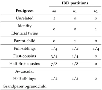
In Table 1 we have represented the values of the IBD partitions for different pedigrees (adapted from (Weir et al., 2006)). Pedigrees are said to belong the same autosomal kinship class if they have the same Jacquard’s coefficients. As an example, half-siblings and
avun-cular are said to belong to the same kinship class since they have both k0 = k1 = 1/2 and
1.5. Statistical Evaluation 18
Table 1: IBD partitions for some pedigrees (adapted from (Weir et al., 2006)).
IBD partitions Pedigrees k0 k1 k2 Unrelated 1 0 0 Identity Identical twins 0 0 1 Parent-child 0 1 0 Full-siblings 1/4 1/2 1/4 First-cousins 3/4 1/4 0 Half-first cousins 7/8 1/8 0 Avuncular Half-siblings Grandparent-grandchild 1/2 1/2 0
2
S TAT E O F T H E A R T
2.1 e x a c t a l g e b r a i c e x p r e s s i o n s
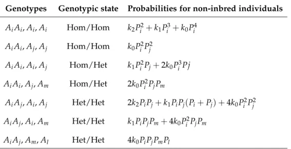
This study will be based on mathematical expressions developed for a pair of non-inbred individuals depending on the frequency of the alleles on the population and on the IBD probabilities of each kinship hypothesis. Such algebraic expressions are presented in the Table 2 (adapted from (Weir et al., 2006)), for unlinked markers and for the simplest assumptions (i.e. absence of mutation and silent allele). Very recently, exact algebraic formulas have been published (Egeland et al., 2017) for a pair of non-inbred individuals, allowing the inclusion of mutations and silent allele.
Table 2: The seven distinct patterns of genotypes that result in seven algebraic expressions, that are possible for two non-inbred individuals and codominant alleles at one autosomal lo-cus (adapted from (Weir et al., 2006)); Pi represents the frequency of the i allele and ks
the s-th IBD partition associated with the pedigree linking the individuals; “Hom” being homozygous and “Het” being heterozygous.
Genotypes Genotypic state Probabilities for non-inbred individuals
AiAi, Ai, Ai Hom/Hom k2Pi2+k1Pi3+k0Pi4 AiAi, Aj, Aj Hom/Hom k0Pi2Pj2 AiAi, Ai, Aj Hom/Het k1Pi2Pj+2k0Pi3Pj AiAi, Aj, Am Hom/Het 2k0Pi2PjPm AiAj, Ai, Aj Het/Het 2k2PiPj+k1PiPj(Pi+Pj) +4k0Pi2Pj2 AiAj, Ai, Am Het/Het k1PiPjPm+4k0Pi2PjPm AiAj, Am, Al Het/Het 4k0PiPjPmPl
Moreover, in Table 3 we present the analytical formulas for testing some biological rela-tionship among three individuals (adapted from (Fung et al., 2006)). So, in the expressions
2.1. Exact Algebraic Expressions 20
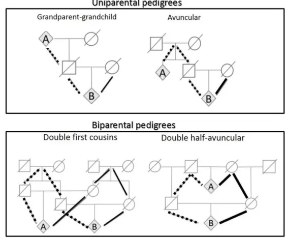
shown in Table 3 we have all the possible joint genotypic probabilities P(X,Y,Z) assum-ing some biological relationship among the three individuals X, Y, and Z. Individuals X and Z are considered as unrelated, X and Y, as well as Y and Z, are assumed as either parent-child, uniparentally related or unrelated. Note that two individuals are considered as uniparentally related if they are related either paternally or maternally (as avuncular or
half-siblings) and thus they are linked through a pedigree for which K2 =0. On the other
hand, biparental pedigree describes individuals related both maternally and paternally (for
which K26=0) - see Figure 4. We can examine the biological relationship between Y and Z
when the biological relationship between X and Y are certainly known. For example, in the paternity testing case we can use the mother who will be X - when there is no doubt that this is the mother, the father will be Z - where the doubt resides, and the child will be Y (Fung et al., 2006).
Figure 4: Examples of uniparental and biparental pedigrees.
These formulas can not always be used. For example, when testing the hypotheses: ”The individuals are related as full-siblings“ versus ”The individuals are related as half-siblings“, or even, ”The individuals are related as full-siblings“ versus ”The individuals
2.2. Software 21
are genetically unrelated“, it is impossible to use them, regardless of the third individual analyzed since the IBD partitions of the full-siblings pedigree, as we can see from Table 1,
are k0 =k2=1/4 and k1 =1/2, and one of the requirements is k2=0.
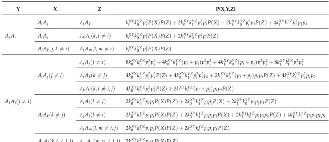
Table 3: The algebraic expressions for testing some biological relationships among three individuals (adapted from (Fung et al., 2006)). The joint genotype probabilities P(X,Y,Z), for all possible genetic configurations of X, Y, and Z.
Y X Z P(X,Y,Z) AiAj AiAk kXY0 kYZ0 p2iP(X)P(Z) +2kXY0 kYZ1 p2ipkP(X) +2kXY1 kYZ0 p2ipjP(Z) +4kXY1 kYZ1 p2ipjpk AiAi AiAj AkAl(k, l6=i) kXY0 kYZ0 p2iP(X)P(Z) +2kXY1 kYZ0 p2ipjP(Z) AjAk(j, k6=i) AlAm(l, m6=i) kXY0 kYZ0 pi2P(X)P(Z) AiAj(j6=i) 8kXY0 kYZ0 p3ip3j+4kXY0 kYZ1 (pi+pj)pi2p2j+4kXY1 kYZ0 (pi+pj)p2ip2j+8kXY1 kYZ1 p2ip2j AiAj(j6=i) AiAk(k6=j) 4k0XYkYZ0 p2ip2jP(Z) +4kXY0 kYZ1 p2ip2jpk+2kXY1 kYZ0 (pi+pj)pipjP(Z) +4kXY1 kYZ1 p2ipjpk AkAl(k, l6=i, j) 4k0XYkYZ0 p2ip2jP(Z) +2kXY1 kYZ0 (pi+pj)pipjP(Z) AiAj(j6=i) AiAl(l6=j) 2kXY0 kYZ0 pipjP(X)P(Z) +2kXY0 kYZ1 pipjP(X) +2kXY1 kYZ0 pipjpkP(Z) AiAk(k6=j) AjAl(l6=i) 2k0XYkYZ0 pipjP(X)P(Z) +2kXY0 k1YZpipjplP(X) +2kXY1 kYZ0 pipjpkP(Z) +4kXY1 kYZ1 pipjpkpl AlAm(l, m6=i, j) 2kXY0 kYZ0 pipjP(X)P(Z) +2kXY1 k0YZpipjpkP(Z) AkAl(k, l6=i, j) AmAn(m, n6=i, j) 2kXY0 kYZ0 pipjP(X)P(Z)
The application of formulas is prone to error, so in more complicated cases it is necessary to resort to programs designed for this purpose.
2.2 s o f t wa r e
There are several programs used to carry out the statistical calculations, such as Fa-milias, PatPCR, Bdgen Simedic or PatCan. One of the most used worldwide is Familias (Mostad et al., 2012). To illustrate this wide usage of this software we present the statistics of the Intercomparison Program of 2015: ”Analysis of DNA polymorphisms in blood stains and other biological samples”, where Familias was the tool used by 69% of the laboratories from the 58 which participated in the advanced level of kinship analyses (Antonio Amorim,
2015). This is an exercise that has been held annually since 1992, organized by The Spanish
and Portuguese Speaking Working Group of the International Society for Forensic Genetics (GHEP-ISFG), with the objective of improving the standardization of methods and encour-aging a meeting point to discuss the analytical strategies and different methodologies used by different laboratories.
2.3. Software Validation 22
Familias (http://www.familias.name) existed for several years exclusively as a Win-dows program to calculate probabilities in connection with the use of DNA data to infer family relationships, but it is now possible to make use of the Familias through R. It is a freeware and it is one of the most used softwares in the world for kinship analyses. In-deed, using the line of code ”install.packages(‘Familias’)“ we can use the functionalities of Familias. It was developed by Petter Mostad, Thore Egeland and Ivar Simonsson and it represents an implementation of an interface to the core Familias functions, which are pro-grammed in C++ (Mostad et al., 2012). Note that, how the command-line runs allows for the analysis of many cases simultaneously, and due to that we was able to lead this work.
Familias is used to compute likelihoods in cases where the DNA profiles of the in-dividuals involved are known, but their kinship is in doubt and comparison between two alternatives is needed. Provided with alternative family constellations (or pedigrees) for the group of people involved, DNA observations for some of the individuals, and a database with allele frequencies in the relevant population, the program calculates several statistics of interest for kinship evaluation, namely the LR previously described. Besides the possibil-ity of inclusion of any pedigree, it allows the incorporation mutation models that are even customizable and silent alleles with specified frequencies for each marker.
2.3 s o f t wa r e va l i d at i o n
While computing the likelihood of all kinship problems linking two and some in case of three individuals (assuming independent transmission, allelic codominance and absence of mutation) can be done resorting to formulae presented in Tables 2 and 3, for more complex cases and/or assumptions, specific software is needed. Indeed, the development of calculations by hand for individual cases becomes, rapidly, a herculean task inadmissibly prone to error. On the other hand, the impact of the likelihood ratio calculating software on the quality of the expert witness report is critical as the wrong or inaccurate calculation or data interpretation, in extreme cases, may lead to false conclusions.
Software validation is the confirmation by examination and provision of objective evi-dence that the particular requirements for a specific intended use are fulfilled. This means that any software, even the simpler ones, should be documented and properly updated (Dr´abek, 2009). Particularly in forensics, it is crucial that the computations which lead to a specific statistical result are able to be re-done at any time. Extended documentation and previous versions of the software should then be available (Gjertson et al., 2007).
2.3. Software Validation 23
Commercial off-the-shelf (COTS) software products for the LR calculation are not suf-ficiently validated, even though this is a well-known statistical technique (Dr´abek, 2009). Accredited laboratories should validate software related to forensic evidence, since it is this software that lead judges to decide on guilt or innocence or to identify a person or kinship. For these reasons, validation must be done, according to pre-established standards, having the International Society for Forensic Genetics (ISFG) published guidelines on this regard. More information about these recommendations can be found in (Coble et al., 2016).
Software, in comparison with machines or instruments, may contain failures without any warning or, during updates, apparently insignificant changes in the code may result in problems in another code location. In addition, even small programs can be complex due to the different answers that they have to give depending on the different inputs (Dr´abek,
2009).
Thereby, software can be likened to “black boxes” since the user can neither access to their content nor, most of the times, to alternative means to replicate the computations. Thus, it is necessary to validate the software to make sure that its use provides a correct result and not a result of an error in its implementation. One possible strategy, wherever possible, is to compare the results obtained using exact algebraic formulas and the results obtained via the software (only possible for some cases and simple assumptions) or com-paring the results given by different softwares with the same assumptions.
Previously to the establishment of ISFG recommendations (Coble et al., 2016) the authors of Familias considered the software validated by the work (Dr´abek, 2009), which comprises seven test cases:
• Classical trio: mother-child-alleged father data with all possible allelic paternity situ-ations inputed;
• Deficiency cases: missing mother case;
• Complicated pedigree: low-resolution genotypes for a Japanese cousin case; • Mutation: trio profiles in cases of paternity inconsistency;
• Silent allele: for mother-child-alleged father;
• Simulation: 100 simulating repeats without null alleles and mutations were performed for sixteen pedigrees based on paternity pedigree;
3
O B J E C T I V E S
In short, and broadly speaking, the objectives outlined for this thesis are:
• For a specific set of kinship problems involving two individuals, where the sharing of genetic information is not required, evaluating the statistical power of the result when: (a.) the number of independent autosomal markers analyzed varies; and/or, (b.) a third individual undoubtedly related to at least one of the two individuals under analysis is considered;
• Validating the software Familias for a set of pedigrees involving only two individuals using exact algebraic formulas and assuming independent autosomal transmission.
4
M AT E R I A L A N D M E T H O D S
4.1 k i n s h i p p r o b l e m s
The analyzed pedigrees that integrate into the kinship problems are Full-siblings (FS), Half-siblings (HS), Avuncular (AV), Unrelated (Unr), First cousins (FC) and Half first cousins (HC). The addressed kinship problems are represented in Figure 5, and the subsets of in-dividuals to be analyzed for each kinship problem are: {A, B}, {A, B, C}, {A, B, D}, and {A, B, E}. Since, for Fig 5(e.) and Fig 5(f.), there is no ”E” individual, only the subsets of individuals: {A, B}, {A, B, C} and {A, B, D} will be considered. Each of the six cases under study has two exhaustive and mutually exclusive hypotheses associated, a priori de-termined, which are represented in Table 4.
Overall, in this thesis, six kinship tests will be carried out with the simulation of 100 000 profiles for each pedigree, where we have the following hypotheses to compare:
• ”A and B are related as full-siblings“ versus ”A and B are related as half-siblings“; • ”A and B are related as full-siblings“ versus ”A and B are genetically unrelated“; • ”A and B are related as half-siblings“ versus ”A and B are genetically unrelated“; • ”A and B are related as avuncular“ versus ”A and B are genetically unrelated“; • ”A and B are related as first cousins“ versus ”A and B are genetically unrelated“; • ”A and B are related as half first cousins“ versus ”A and B are genetically unrelated“.
4.2. Database 26
Figure 5: Representation of the six cases under study.
Table 4: The hypotheses to be compare that derive from Figure 5.
Figure 5 Hypotheses Description
(a.) H0 {A, full sister of D, daughter of mother C, and paternal granddaughter of E, is full sister of B}
H1 {A, full sister of D, daughter of mother C, and paternal granddaughter of E, is maternal half-sister of B} (b.) H0 {A, full sister of D, daughter of mother C, and paternal granddaughter of E, is full sister of B}
H1 {A, full sister of D, daughter of mother C, and paternal granddaughter of E, is unrelated of B} (c.) H0 {A, full sister of D, daughter of mother C, and paternal granddaughter of E, is paternal half-sister of B}
H1 {A, full sister of D, daughter of mother C, and paternal granddaughter of E, is unrelated of B} (d.) H0 {A, full sister of D, daughter of mother C, and sister-in-law of E, is aunt of B}
H1 {A, full sister of D, daughter of mother C, and unrelated of E, is unrelated of B} (e.) H0 {A, granddaughter of D, daughter of mother C, is first cousin of B}
H1 {A, granddaughter of D, daughter of mother C, is unrelated of B} (f.) H0 {A, granddaughter of D, daughter of mother C, is half first cousin of B}
H1 {A, granddaughter of D, daughter of mother C, is unrelated of B}
4.2 d ata b a s e
The genotypic configurations were obtained considering a Norwegian database for 35
independent Au-STRs 1
(Dupuy et al., 2013). The population frequency database used comprises the genetic information from 9586 unrelated Norwegians as well as individuals
1 Complete set of the 35 Au-STRs analyzed: D3S1358, TH01, D21S11, D18S51, PENTA E, D5S818, D13S317, D7S820, D16S539, CSF1PO, PENTA D, VWA, D8S1179, TPOX, FGA, D19S433, D2S1338, D10S1248, D1S1656, D22S1045, D2S4414, D12S391, SE33, D7S1517, D3S1744, D2S1360, D6S474, D4S2366, D8S1132, D5S2500, D21S2055, D10S2325, D17S906, APOAI1 and D11S554.
4.3. Simulation of genetic profiles 27
from three immigrant populations from East Africa, East Asia and Middle Asia in a total of 1531 individuals (Dupuy et al., 2013).
Throughout this study, 5 subsets of autosomal markers will be analyzed. These subsets were formed based on the number of autosomal markers comprised - 17, 22, 27, 32 and 35. The division was performed by order, that is, for example the set of 22 markers consists of
the set of markers starting at the 1stmarker of the list: D3S1358, and ending at 22nd marker
of the list: D12S391. The complete ordered set of 35 Au-STRs is found in f ootnote1.
The goal of creating these 5 subsets is the understanding of the correlation between the statistical power of the result with the number of independent markers analyzed (and to obtain guidance for a future theoretical treatment of the problem).
4.3 s i m u l at i o n o f g e n e t i c p r o f i l e s
The R language (R Core Team) is used by scientists, statisticians and, more recently, by data scientists as a convenient tool for exploratory analysis of interactive data. R is provided with a lot of pre-installed packages, but still allows adding specific packages. Furthermore, it offers a wide variety of statistics and graphical techniques. Therefore, R language will be used to implement the code needed in this work.
The genetic profiles represented in Figure 5 were generated, R language was used to sim-ulate 100 000 of each and the information about the individuals of interest {A,B,C,D,E} was stored. This generation of genetic profiles consisted of using a table with the frequencies of the alleles by genetic markers, mentioned in section 4.2.
As an example, the Full-Siblings pedigree was simulated resorting to the generation of a pair of unrelated individuals (the mother and the father) and taking into account the frequencies of the alleles in the population. Resorting to accumulated frequencies and a random number between 0 and 1, alleles with greater frequencies were more likely to be selected as belonging to individuals’ genotypes. Then, the genotype of each of their children was obtained assuming that each of the parents transmitting one or other allele is equally likely. For computations considering a pair of individuals, only the genotypes of the full-siblings were considered.
4.4. Validation of Familias for the simplest assumptions - absence of mutation and presence of silent allele 28
• Validation of Familias for the simplest assumptions - absence of mutation and
silent allele: only the individuals represented in Figure 5 as A and B are analyzed, not considering mutations or silent allele - detailed description in section 4.4.
• Measurement of the impact of considering a third individual and/or a greater
num-ber of markers: the sets of individuals - {A,B}, {A,B,C}, {A,B,D} and {A,B,E} - are analyzed taking into account mutations and silent allele with different sets of ana-lyzed markers - detailed description in section 4.5.
4.4 va l i d at i o n o f f a m i l i a s f o r t h e s i m p l e s t a s s u m p t i o n s - absence of
mu-tat i o n a n d p r e s e n c e o f s i l e n t a l l e l e
The formulas presented in Table 2 were implemented and, additionally, code that al-lowed the choice of the respective formula was used, since there are seven formulas and its choice depends on whether the individuals are, for each marker, homozygous or het-erozygous and on the number of shared alleles. For all the cases under study presented in Figure 5, using the 100 000 profiles generated and the formulas implemented, partial LR tables were obtained for 35 autosomal markers.
In order to make a comparison of the results obtained with the implementation of the formulas present in Table 2 and those obtained with Familias, using the same profiles and the same conditions, we proceed to the respective computations.
Additionally, to validate the results of Familias with those of the formulas already pub-lished, we will obtain the maximum errors per case study. So, to obtain the maximum error for each case under study, the two tables of the partial LRs were used, one considering the use of the implemented formulas (Table 2) and other considering the use of the Familias package, computing the difference between both and finding the maximum value.
4.5 m e a s u r e m e n t o f t h e i m pa c t o f c o n s i d e r i n g a t h i r d i n d i v i d ua l a n d/or
a g r e at e r n u m b e r o f m a r k e r s
A set of R scripts making use of Familias were created to obtain partial LR tables, and then, by the called ’product rule’ described in subsection 1.5.2, results for the final LR value were performed considering the several sets of markers {17, 22, 27, 32 or 35} and a genetic profile of a third individual {C, D or E}, where C, D and E are assumed to undoubted relatives of A or B. The same database (Dupuy et al., 2013) will be used with the frequency of alleles per marker. The pairwise comparisons under study will also be the same (Figure