Atmospheric circulation and climate of the Euro-Atlantic sector since 1685 based on new directional flow indices

(1)

2019

Atmospheric circulation and climate of the Euro-Atlantic sector since

1685 based on new directional flow indices

“ Documento Definitivo”

Doutoramento em Ciências Geofísicas e da Geoinformação Especialidade de Meteorologia

Javier Mellado-Cano

Tese orientada por: Dr. Ricardo Machado Trigo

Dr. David Barriopedro

(2)

(3)

2019

UNIVERSIDADE DE LISBOA FACULDADE DE CIÊNCIAS

Atmospheric circulation and climate of the Euro-Atlantic sector since 1685 based on new directional flow indices

Doutoramento em Ciências Geofísicas e da Geoinformaçao Especialidade de Meteorologia

Javier Mellado-Cano

Tese orientada por: Dr. Ricardo Machado Trigo

Dr. David Barriopedro

Júri: Presidente:

● João Manuel de Almeida Serra, Professor catedrático e Presidente do Departamento de

Engenharia Geográfica, Geofísica e Energía da Faculdade de Ciências da Universidade de Lisboa Vogais:

● Doutor David Barriopedro Cepero, Research Scientist do Instituto de Geociencias da Universidad Complutense de Madrid, Espanha

● Doutor José Manuel Vaquero Mártinez, Professor Titular do Centro Universitario de Mérida da Universidad de Extremadura, Espanha

● Doutor David Gallego Puyol, Professor Titular da Facultad de Ciencias Experimentales da Universidad Pablo de Olavide, Sevilha.

● Doutor Pedro Miguel Ribeiro Sousa, Investigador Pós Doutoramento no Instituto Dom Luiz da Universidade de Lisboa

Documento especialmente elaborado para a obtenção do grau de doutor

(4)

(5)

i

Acknowledgements

I would like to thank all people involved in this thesis.

First of all, I would like to acknowledge Dr. Ricardo Machado Trigo for giving me the opportunity to live this adventure in Lisbon and write this PhD thesis in the University of Lisbon. He was always a supporting supervisor of this thesis and a great leader of the Climate variability and Climate Change Group at Instituto Dom Luiz.

A good deal of the research themes in this work is due to Dr. David Barriopedro. He was first the advisor of my master and now also PhD thesis. Thank you for all the critical examinations, discussions, corrections and endless things that are impossible to express in words. Today I am finishing a PhD thanks to everything you have taught me. You have always been, and you will always be a scientific’ model for me.

In fact, the person who started this adventure was Ricardo Garcia-Herrera. Among many things, he showed me that I have to believe in my results and that all the results can always be put in a sexier way. Thank you for your experience and support throughout this long ride.

A special thanks goes to the STREAM group, although throughout this process I have never been an official part of it, unofficially you made me feel like part of this big family. I would also like to express my gratitude to the Climate change, atmosphere-land-ocean processes and extremes group from IDL that accommodated me during these years. A little part of this adventure took place in Germany; I would like to thank the Climatology, Climate Dynamics and Climate Change group from the University of Giessen, in particular Professor Jürg Luterbacher, for opening the doors of their castle and give me the opportunity to live and work for some months in Giessen.

(6)

I am especially grateful to the Oompa Loompas (Antonio, Fernando, Froila, Jose and Maddalen) at the 220 office, for their friendly shoulder when I needed it. Big thanks goes to my PhD colleagues Rodrigo and Ana. Living in a foreign country, far for home, is not always easy. In my case, you are the people who have made Lisbon a home for me. Very special thanks goes to my friends near and far. They know who they are, and I am very thankful for all your time and support.

I would have not gotten this far if it was not for my family. During this long journey many of you have passed away, although you never understood very well what I was doing so far from you. I know that wherever you are, you are proud of me as much as I am of being your grandson and nephew. You will live as much as my memories do.

The greatest of the thanks to my sister and parents for all their love, support and distraction. All three of you are my idols. I have become who I am thanks to you.

Last but not least, my most sincere thanks goes to the serendipity of this journey. Esther, you observed and lived this ride of emotions with me, thanks for giving me the peace and balance that I need. Thank you for believing in me and for seeing always the best part of me. You are and you will always be a source of inspiration to me, without you I would not have made it.

(7)

iii

Abstract

Knowledge of atmospheric circulation beyond the mid-18th century is hampered by the scarcity of instrumental records, particularly over the Ocean. In this regard, wind direction observations kept in ships’ logbooks are a consolidated but underexploited instrumental source of climatic information.

In this Thesis we present four monthly indices of wind persistence, one for each cardinal direction, based on daily wind direction observations taken aboard ships over the English Channel. These Directional Indices (DIs) are the longest observational record of atmospheric circulation to date, covering the 1685-2014 period. DIs anomalies are associated with near-surface climatic signals over large areas of Europe in all seasons, being excellent benchmarks for proxy calibrations.

DIs series are dominated by large interannual-to-interdecadal variability and provide all year-round observational evidences of atmospheric circulation responses to external forcings (tropical volcanic eruptions) or the role of the atmospheric circulation in anomalous periods such as the Late Maunder Minimum (LMM, 1675-1715). In both cases, the results emphasize complex patterns that are more heterogeneous than previously thought, with contrasting spatial signals in both circulation and temperature.

When considered together, DIs explain a considerable amount of European climate variability, improving that accounted for by single modes of variability. This allows us to yield the longest instrumental-based series of the winter North Atlantic Oscillation (NAO) and East Atlantic (EA). The results highlight the role of EA in shaping the North Atlantic action centers and the NAO’s European climate responses. Transitions in the NAO/EA phase space have been recurrent and explain non-stationary NAO signatures and anomalous periods. NAO and EA have additive effects on the jet speed but opposite impacts on the jet latitude, allowing us to derive the first instrumental reconstruction of the North Atlantic eddy-driven jet stream for the last three centuries.

Keywords: Ships’ logbooks, Euro-Atlantic atmospheric circulation, North Atlantic Oscillation, Jet Stream, Past European Climate.

(8)

(9)

v

Resumo

O conhecimento relativo à circulação atmosférica antes de meados do século XIX está condicionado pela escassez de registos instrumentais, em particular sobre os oceanos. Os diários de bordo de navios representam uma fonte privilegiada de observações meteorológicas sobre os oceanos e mares relativamente a este período pré-instrumental. Em particular, os registros de direção do vento são uma fonte consolidada, mas sub-explorada, de informação climática homogénea, medida com uma bússola ao longo de vários séculos. Algumas regiões com intensa actividade marítima, como o Canal da Mancha (English Channel) podem proporcionar observações contínuas relativamente às condições atmosféricas em áreas estratégicas, nomeadamente as latitudes médias do oceano Atlântico, desempenhando um papel importante na definição das condições climáticas da Europa.

Nesta tese apresenta-se uma metodologia robusta de forma a obter quatro índices mensais de persistência do vento, um para cada direção cardinal: Norte, Este, Sul e Oeste, baseados em observações diárias de direção do vento registadas em embarcações que navegavam o Canal da Mancha. Até à data, estes índices direcionais representam o registo observacional mais longo da circulação atmosférica, cobrindo o período 1685-2014. As anomalias destes índices refletem sinais climáticos sobre áreas extensas da Europa em todas as estações do ano. Em geral, valores anómalos dos índices zonais (de Oeste e Leste) e meridionais (de Norte e de Sul) afetam diferentes regiões da Europa. Os sinais de precipitação são fortemente controlados pela advecção da humidade, principalmente influída pelos índices zonais, e apresentam uma resposta robusta e coerente ao longo do ano. De maneira distinta, a resposta espacial da temperatura é explicada pela advecção da temperatura e processos radiativos. Consequentemente, o sinal de temperatura associado aos índices zonais inverte durante o verão.

Modelos estatísticos que incluam como preditores todos os índices direcionais são capazes de explicar uma boa fração da variabilidade climática europeia, melhorando em muitos casos aqueles baseados apenas na Oscilação do Atlântico Norte (NAO, North Atlantic Oscillation). Alem disso, os índices direcionais mostram potencial para constringir a resposta da circulação atmosférica a forçamentos externos e as anomalias climáticas associadas. Em particular, são fornecidas evidências instrumentais de sinais de circulação atmosférica ao longo de todo o ano na sequência de fortes erupções vulcânicas tropicais ocorridas nos últimos três séculos.

(10)

Estas respostas sugerem que o testemunhado aquecimento invernal, bem como o arrefecimento do verão depois de uma erupção, podem ser detetados com vários meses de antecedência.

O início dos registos utilizados neste trabalho (1685-1715) coincide com as últimas décadas do Mínimo de Maunder (ca., 1645-1715), um dos períodos mais frios na Europa que persistiu por várias décadas. Uma análise baseada nos índices direcionais demonstrou que a circulação de inverno foi a que mais contribuiu para as condições generalizadas de frio que caracterizaram as três últimas décadas desse período. No entanto, o período na Europa foi mais heterogéneo do que anteriormente se pensava, exibindo padrões espaciais contrastantes tanto na circulação atmosférica como nas anomalias do campo da temperatura e uma considerável variabilidade decadal. Em particular, é demonstrado um aumento dos ventos de Norte na primeira metade do período (1685-1700) que favoreceram invernos mais frios, enquanto na segunda metade (1700-1715) a predominância dos ventos de Sul contribuíram para condições mais amenas.

Os índices direcionais permitiram a obtenção de um novo e completo catálogo com as características dinâmicas de todos os invernos para o período 1685-1715. Neste contexto, a temperatura inferida a partir da circulação atmosférica confirma a maioria dos invernos extremamente frios bem testemunhados na literatura existente para este período. No entanto esta análise cuidada também permitiu revelar outros invernos bastante frios mas pouco descritos como tal na literatura, bem como uma quantidade substancial de invernos amenos que passaram desapercebidos até agora. Os resultados sugerem uma não estacionariadade do padrão da NAO dentro do período considerado (1685-1715) explicando as discrepâncias entre o comportamento extremo ou ameno, em termos de temperatura, de alguns dos invernos. Outro resultado central deste trabalho foi a possibilidade de, com base nos índices direcionais, construir a mais longa reconstrução observacional dos dois modos principais de variabilidade atmosférica no inverno no setor Euro-Atlântico, isto é da North Atlantic Oscillation (NAO) e o da East Atlantic pattern (EA). A identificação de tipologias de invernos através de combinações da NAO e da EA durante o século XX sublinham o papel da EA na alteração de centros de ação no Atlântico Norte e na influência que exerce nas respostas climáticas da NAO. A modulação do impacto climático da NAO, em função da fase e intensidade da EA, é verificada de uma forma mais intensa no campo da precipitação do que no da temperatura, afetando de forma significativa áreas extensas com respostas fortes à NAO, tais como a Gronelândia e algumas regiões no Mediterrâneo. Isto impede o uso de relações simplistas

(11)

vii

estabelecidas entre proxies naturais da NAO provenientes da Gronelândia, Ibéria, Balcãs ou Turquia.

Além disso, os resultados para o século XX indicam que a NAO e a EA têm um sinal forte na corrente de jato do Atlântico Norte: a NAO e a EA têm efeitos aditivos na velocidade do jato, sendo maior o sinal da NAO, e efeitos opostos comparavelmente importantes na latitude preferencial do jato. Portanto, as maiores anomalias na velocidade do jato tendem a ocorrer em invernos com fases de igual fase para ambos os modos, enquanto as maiores divergências na latitude do jato ocorrem em invernos com fases opostas. Estas relações recentes são exploradas para reconstruir a evolução das principais características do jato ao longo dos três últimos séculos. Os resultados mostram uma variabilidade substancial na corrente de jato do Atlântico Norte tanto à escala inter-anual como à escala inter-decadal, fornecendo novas evidências das dinâmicas por detrás de alguns períodos anómalos. Esta variabilidade asocia-se a períodos dominados por combinações específicas da NAO e a EA. Transições entre diferentes combinações de fase de ambos os modos têm sido recorrentes e explicam as assinaturas não-estacionárias da NAO, tal como o deslocamento dos seus centros de ação no final do século XX e também algumas divergências observadas entre índices históricos da NAO.

Em resumo, este conjunto de resultados promissores evidenciam o valor acrescido dos índices direcionais construídos através de registros instrumentais de bordo de embarcações. No contexto de trabalho futuro, a sua natureza instrumental, elevada resolução temporal e origem marítima faz com que sejam uma excelente referência para compreender a variabilidade da circulação atmosférica e melhorar reconstruções atuais do clima europeu nos últimos séculos.

Palavras-chave: Diários de bordo de embarcações, circulação atmosférica Euro-Atlântica, North Atlantic Oscillation, Corrente de jato, Clima Europeu passado.

(12)

(13)

ix

List of Acronyms and Abbreviations

20CR 20th century: the Twenty Century Reanalysis

AH Azores High

ASM Australian Summer Monsoon

BARCAST Bayesian Algorithm for Reconstructing Climate Anomalies in Space and Time

CET Central England Temperature

CLIWOC Climatological Database for the World's Oceans

CMIP Coupled Model Intercomparison Project

CMIP5 Coupled Model Intercomparison Project (phase 5)

CPC Climate Prediction Center

CRU Climate Research Unit

DIs Directional Indices

DJF December, January, February

EA East Atlantic pattern

ECMWF European Centre for Medium Range Weather Forecast

EI Easterly Index

GPCC Global Precipitation Climatology Center HadISST Hadley Centre Global Sea Ice and Sea Surface

HLUK Historical Logbooks from United Kingdom

ICOADS International Comprehensive Ocean-Atmosphere Data set

IL Iceland Low

INCITE Instrumental Climatic Indexes Application to the study of the monsoon Mediterranean Teleconnection

ISM Indian Summer Monsoon

ISPD International Surface Pressure Databank

IVMFC Vertically Integrated Moisture Flux Convergence

JJA June, July, August

LIA Little Ice Age

LMM Late Maunder Minimum

MAM March, April, May

MCA Medieval Climate Anomaly

MM Maunder Minimum

(17)

xiii

MSEC Mean Squared Errors of Climatology

MSSS Mean-Squared Skill Score

NAO North Atlantic Oscillation

NCAR National Center for Atmospheric Research NCEP National Centers for Environmental Prediction

NGDC National Geophysical Data Center

NI Northerly Index

NOAA National Oceanic and Atmospheric Administration

NWI Northerly Wind Index

RECLAIM RECovery of Logbooks And International Marine data

RMSD Root Mean Square Difference

SCA Scandinavian pattern

SEA Superposed Epoch Analyses

SI Southerly Index

SLP Sea Level Pressure

SNAO High-summer North Atlantic Oscillation

SON September, October, November

SRM Stepwise Regression Model

SVD Singular Value Decomposition

VEI Volcanic Explosivity Index

WAM West African Monsoon

WI Westerly Index

WNPDI Western North Pacific Directional Index

(18)

List of Figures

Figure 1.1. Non-robustness of the predicted circulation response to climate change. Lower

tropospheric (850 hPa) wintertime zonal wind speed (grey contours, 5 ms−1 spacing) over the North Atlantic, and the predicted response to climate change over the twenty-first century under the Representative Concentration Pathway 8.5 scenario (color shading), from four different CMIP5 models, averaged over five members from each model ensemble. Stippling (density is proportional to grid spacing) indicates regions where the climate change response is significant at the 95% level based on the five ensemble members. From Shepherd 2014 ... 2

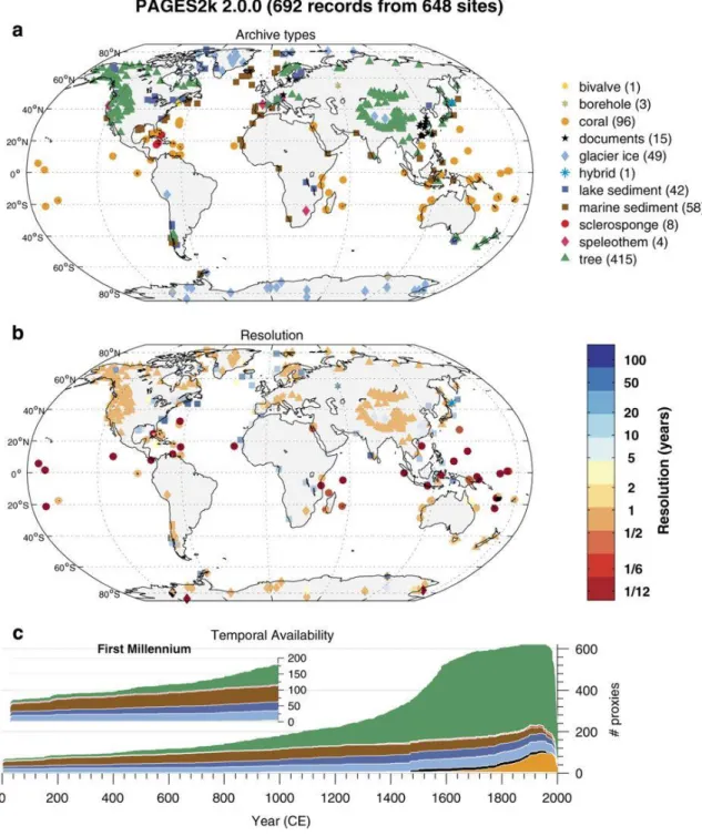
Figure 1.2. Spatiotemporal data availability in the PAGES2k database. (a) Geographical distribution,

by archive type, coded by color and shape. (b) Temporal resolution in the PAGES2k database, deﬁned here as the median of the spacing between consecutive observations. Shapes as in (a), colors encode the resolution in years (see colorbar). (c) Temporal availability, coded by color as in (a). ... 4

Figure 1.3. Observed and simulated time series of the anomalies in annual and global mean surface

temperature. All anomalies are differences from the 1961–1990 time-mean of each individual time series. The reference period 1961–1990 is indicated by yellow shading; vertical dashed grey lines represent times of major volcanic eruptions. Single simulations for CMIP5 models (thin lines); multi-model mean (thick red line); different observations (thick black lines). Adapted from Flato et al. 2013 ... 6

Figure 1.4 Tambora eruption (Apr 1815) and the simulated tropical Pacific surface temperature

anomalies (°C) during winter 1816 for the 15 CESM-LME simulations that include volcanic forcing. The Dec–Feb (DJF) seasonal surface temperature anomalies for each simulation with volcanic forcing shown here are computed relative to each simulation’s long-term annual cycle. Taken from Otto-Bliesner et al. (2016). ... 7

Figure 1.5 Left panel: printed page of Bento Sanches Dorta weather observations of February 1785 in

Rio de Janeiro (Brazil) (Sanches Dorta 1799b, p. 380) (Farrona et al. 2012); Right panel: complete description of the solar eclipse observation sequence realized by Dorta on February 9th of 1785 in Rio de Janeiro (Brazil). From Vaquero et al. 2005 ... 8

Figure 1.6. Approximate earliest date of continuous instrumental records. From Bradley 2011 ... 9 Figure 1.7. Left column: logbook’ page from the Creoula, a training ship of the Portuguese Navy, of

the year 2015. Right column: logbook’ page from the Spanish Brig S. Francisco Javier (La suerte) of the year 1796. ... 10

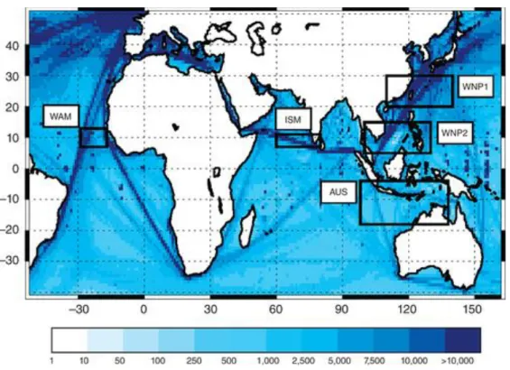
Figure 1.8. Number of wind direction observations in a 1 × 1 grid for the 1800–2014 period available

in ICOADS 3.0. Black rectangles (labeled by white boxes) indicate the areas selected to compute monsoonal indices. From García-Herrera et al. 2018 ... 12

Figure 1.9. Monsoon Instrumental Climatic Indexes developed in the context of the INCITE project

using ICOADS 3.0 for a) the African Summer Monsoon (AMS), b) The Australian Summer Monsoon, c) the Western North Pacific Summer Monsoon and, d) date of the Indian Summer Monsoon onset. Shaded smoothed curves are computed as a robust locally weighted regression with a 21-year window width (Cleveland, 1979). From García-Herrera et al. 2018. ... 13

Figure 1.10. Main modes of atmospheric variability over the Euro-Atlantic sector for winter

(19)

xv

correlation maps between the seasonal time series of the indices and geopotential height at 500 hPa for the 1951-2018 period. ... 15

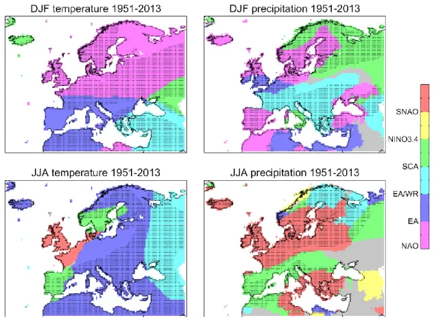
Figure 1.11 Spatial distribution of the dominant modes of atmospheric variability influencing

temperature (left panels) and precipitation (right panels) interannual variations during winter (DJF, top panels) and summer (JJA, bottom panels) seasons of the 1950–2014 period. Colors identify the teleconnection pattern with the largest Pearson (Spearman) correlation coefficient with seasonal-mean temperature (precipitation) data. Dotted (grey shaded) regions identify areas where more than one (none) mode of variability displays significant correlations at the 95% confidence level. The following: NAO, EA, East Atlantic/Western Russian pattern (EA/WR), SCA, ENSO and the high-summer NAO (SNAO). Adapted from García-Herrera and Barriopedro (2018). ... 16

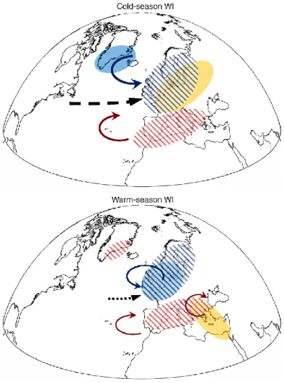
Figure 1.12. Schematic displaying the main signatures in atmospheric circulation (arrows),

temperature (filled shading) and precipitation (hatching) associated with positive phases of the Westerly Index in: top) cold seasons (herein referred to all seasons, except for summer); bottom) warm season (June-to-august). Solid arrows denote enhanced cyclonic (in blue) and anticyclonic (in red) circulation, with dashed arrows indicating the intensity of the westerlies. Orange/blue shading denotes anomalously warm / cold temperatures. Red/blue hatching indicates regions with reduced/increased precipitation. From García-Herrera et al. 2018 ... 19

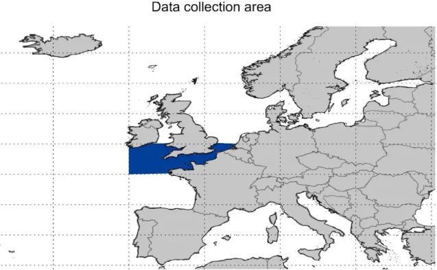
Figure 2.1. Area of analysis. Blue shading shows the selected region for the collection of wind

direction observations during the period 1685-2014 ... 23

Figure 2.2. (a) Monthly time series of the areal-average magnetic declination (in º from true north)

over the English Channel (solid line). Dots indicate historical monthly observations of the magnetic declination from London (red; Malin and Bullard 1891)) and Paris (blue; Hartmann et al. 2013); (b)Total number of daily windy observations retained (1662-2014) over a regular grid of 0.25ºx0.25º in longitude-latitude in English Channel ... 26

Figure 2.3. (a) Annual time series with the daily mean frequency of wind direction observations over

the English Channel (in # per day) from Royal Navy Ships’ logbooks and ICOADS V3.0; b) Monthly time series showing the percentage of days with missing data (grey line) along the 1685–2014 period. The black line depicts a 12-month running average. ... 28

Figure 3.1 Averaged correlations between 1000 randomly degraded DIr series computed with only

one wind record per day and the DIp series computed from a minimum percentage pd (x-axis, ranging from 1 to 95%) of wind records with a d-wind direction over the English Channel: a) NI; b) EI; c) SI and; d) WI. Lines (shading) indicate the mean correlation (full range of correlations) obtained from the 1000 random DIr series for different sub-periods (see legend). The vertical dotted line identifies the pd threshold value adopted for each DI. ... 41

Figure 3.2 Annual time series of the accumulated frequency of different types of conflicts and

undefined wind days (in % with respect to the total number of days of the analyzed period). ... 43

Figure 3.3. Distribution of estimated uncertainties of the DIs as a function of the total number of

monthly observations (in percentage of days in the month): a) NI; b) EI; c) SI and; d) WI. Colored lines represent the four seasons (see legend in panel b). ... 45

Figure 3.4. Standardized seasonal series of DIs for 1685-2014 (blue line) with the associated

uncertainty (grey shading, ± sigma). Vertical blue bars indicate years with at least one missing month. ... 46

Figure 3.5. Distribution of the SC parameter value as a function of the number of breakpoints in the

(20)

of breakpoints in the corresponding DI series, with their locations shown in the lower right corner of each panel. ... 48

Figure 4.1. a) Annual cycle of the DIs for 1685-2014, expressed in percentage of days of each month

with wind blowing from that direction. Red (Blue) lines indicate the 75th₍₂₅th_{) percentile; b) Seasonal}

and annual mean values of the DIs for 1685-2014, expressed in percentage of days of the month with wind blowing from that direction: NI (blue), EI (green), SI (orange) and WI (red) with error bars indicating the ± 1 sigma interval. ... 52

Figure 4.2. Winter (a-d) and summer (e-h) differences between scaled anomaly composites for high

(>1 SD) and low (< -1 SD) DIs. The following variables are shown: geopotential height at 500 hPa (Z500, contours), land near-surface temperature (shading), 500 hPa wind (arrows) and 500 hPa temperature advection (hatching). All units are dimensionless. Solid (dashed) contours represent positive (negative) values, with thick lines indicating significant differences from climatology at p<0.1. Only temperature differences that are significant at p<0.1 are shown. Cross-hatched areas with lines orientated 45º/-45º from the east indicate significant (p<0.1) warm/cold temperature advection. The size of the arrows is proportional to the magnitude of the 500 hPa wind anomaly (a reference value is shown in the bottom right corner of each panel). For better readability, hatched areas (arrows) are only displayed over land (ocean). Numbers in the left bottom corner of each panel represent the number of cases employed in the composite for high / low DIs. Significance is assessed with a 1000-trial bootstrap test. ... 54

Figure 4.3. As Figure 2 but for the following variables: storm tracks (2–5 high pass filtered Z500

variance, contours), land precipitation (shading), 1000–500 hPa vertically integrated moisture transport (arrows) and 1000–500 hPa moisture convergence (hatching). All units are dimensionless. Solid (dashed) contours represent positive (negative) values, with thick lines indicating significant differences from climatology at p<0.1. Only precipitation differences that are significant at p<0.1 are shown and gridpoints with climatological mean precipitation below 10 mm are omitted. Cross-hatched areas with lines orientated 45º/-45º from the east indicate significant (p<0.1) moisture divergence/convergence. The size of the arrows is proportional to the magnitude of the moisture transport anomaly (a reference value is shown in the bottom right corner of each panel). For better readability, hatched areas (arrows) are only displayed over land (ocean). Numbers in the left bottom corner of each panel represent the number of cases employed in the composite for high / low DIs. Significance is assessed with a 1000-trial bootstrap test. ... 56

Figure 4.4. As Figure 4.2 but for spring (a-d) and autumn (e-h). ... 58 Figure 4.5. As Figure 4.3 but for spring (a-d) and autumn (e-h) ... 59 Figure 4.6. Stepwise regression model for the period 1901-2014 showing the best DIs predictors of

seasonal: (a-h) temperature and; (i-p) precipitation anomalies. The best predictor of each season is shown in panels (a-d) for temperature and (i-l) for precipitation. Panels (e-h) and (m-p) indicate the second best predictor of temperature and precipitation, respectively. Rows indicate the respective season from winter (DJF, first row) to autumn (SON, last row). Colors represent the DI: NI (orange), EI (red), SI (green) and WI (blue). White areas show regions where none of the DIs is able to explain a significant amount of variance. ... 61

Figure 4.7. Explained variance (in percentage) of seasonal: (a-h) temperature and; (i-p) precipitation

anomalies based on Stepwise Regression Models for 1901-2014 using the DIs only (panels (a-d) for temperature and (i-l) for precipitation) and the DIs + NAO ((e-h) for temperature and (m-p) for precipitation) as predictors. White areas denote regions where none of the predictors is able to explain a significant amount of variance. ... 63

(21)

xvii

Figure 4.8. Standardized annual series of DIs for 1685-2014 (black line) with the associated

uncertainty (grey shading, ± 1 sigma) and an 11-year running mean (grey line) superimposed. Green/orange shading highlights periods above/below the 1685-2014 mean. Horizontal lines indicate ±1.5 sigma relative to the 1685-2014 period. Vertical blue bars indicate years with at least one missing month. ... 65

Figure 4.9. Frequency difference of positive minus negative seasonal DIs extremes for running

11-year intervals of the 1685-2014 period (x-axis), with red (blue) shading denoting positive (negative) differences. Positive (negative) DIs extremes are defined as those above the 95th (below the 5th) percentile of their seasonal 1685-2014 distribution. Seasons are displayed from the top (winter, DJF) to the bottom (autumn, SON) in the left y-axis. For each season, the DIs are arranged clockwise from the NI (top of each season) to the WI (bottom of each season), as shown for the winter season in the right y-axis. ... 67

Figure 4.10. Superposed epoch analyses of the seasonal standardized DIs following the strongest

(VEI≥5) tropical volcanic eruptions of 1685-2014. For each DI (colored bars, see legend) and season, anomalies are expressed as the difference between the largest standardized anomaly of the years 0 and +1 and the averaged value for the five years preceding each volcanic eruption. Columns with dotted top bars indicate significance at the 90% confidence level after a 5000-trial bootstrap test. Error bars indicate the ±0.5·sigma level. ... 72

Figure 4.11. Reconstructed mean seasonal anomalies (with respect to 1901-2014) of: (a-d):

temperature (ºC) and; (e-h) precipitation (in percentage of normal) following explosive tropical volcanic eruptions of 1685-2014. Red/blue colors indicate positive/negative temperature anomalies and below-/above-normal precipitation. The reconstructed anomalies are derived by applying the Stepwise Regression Model of the DIs series for 1901-2014 to the DIs anomalies recorded after each volcanic eruption. White areas show regions where none of the DIs is able to explain a significant amount of variance. Hatching indicates regions for which 66% of the volcanic eruptions display an anomaly of the same sign. See text for details. ... 73

Figure 5.1. Standardized winter DIs time series for the LMM (1685-1715), with dark (light) grey bars

highlighting years with values above (below) the 1981-2010 average. ... 78

Figure 5.2. Seasonal frequencies of DIs (in percentage of total days) averaged for the LMM (color

bars). Grey thin bars indicate the corresponding value for the 1981-2010 reference period. Grey bars with dotted tops indicate significance differences between the two periods at the 90% confidence level after a two-tailed t-test. ... 79

Figure 5.3. Monthly mean 8-point wind-roses for the LMM: a) December; b) February; c) March. The

frequencies are expressed in percentage of days (contour interval of 8%) with orange (green) colors highlighting wind directions whose frequency is significantly above (below) that of the 1981-2010 period at the 90% confidence level. The climatology of the 1981-2010 period is shown with thick lines. ... 82

Figure 5.4. Monthly mean 8-point wind roses for the first (1685-1699, blue) and second (1700-1715,

red) half of the LMM: a) December; b) January; c) March. Purple indicates the overlapped areas between both subperiods. For a better comparison, the frequency of each bin is expressed in percentage of normals with respect to 1981-2010 (contour interval of 40%). ... 83

Figure 5.5. Scatter plot of the cumulative index (CI) for: a) the LMM winters; b) winters of the

reference period (1981-2010), with colors indicating the year within the LMM. The x-axis (y-axis) represents the CIT (CIC) coordinate of the CI. ... 84

(22)

Figure 5.6. As Figure 5.5a but with open blue squares (red triangles) representing winters of the

cluster one (two). The number of winters of each cluster is shown in the lower right corner. Black symbols denote the centroid CI values of the cluster one (black square, CIT = −2.55, CIC = 0.17) and two (black triangle, CIT = 1.25, CIC = 1.81). Symbols filled with blue (red) in b) represent well documented cold (warm) winters in the literature. ... 86

Figure 5.7. LMM mean winter anomalies with respect to 1981-2010, as inferred from circulation

analogues of the 1901-2014 period: a) near-surface temperature (in ºC); b) precipitation (in percentage of totals). ... 88

Figure 5.8. Winter composites of near-surface temperature (shading, in ºC) and geopotential height

at 500 hPa (contours, in dam) anomalies for the winter analogues of: a) Group 1 (G1); b) Group 2 (G2); c) Group 3 (G3); d) the difference between G2 and G3. Dotted areas highlight those regions where the MSSS is significantly above the climatology at the 90% confidence level. Numbers at the left bottom of each panel indicate the total number of winters of each group. ... 91

Figure 5.9. As Figure 5.8 but for the average of the best analogues of each winter of Group 4: a)

1693; b) 1700; c) 1709. See text for details. ... 93

Figure 6.1. Winter composite differences between positive (>0.5 SD) and negative (<-0.5 SD) phases

of a, c): NAODI (upper panel ) and b, d): EADI (lower panel) for 1901-2010: a, b) near-surface

temperature (shading, in ºC) and geopotential height at 500 hPa (contours, in dam) anomalies; c, d) precipitation (shading, in percentage of normals) and SLP (contours, hPa) anomalies. Only temperature and precipitation anomalies that are significantly different (p<0.05) from the climatology are shown, after a 5000-trial bootstrap test. We used monthly near surface temperature from the CRU TS v3.23 (Harris et al. 2014) and total monthly precipitation from the GPCC (Schamm et al. 2014) on a grid of 1°x1°, as well as geopotential height data at 2.5°x2.5° from the ERA-20C reanalysis (see Section 2.1.2.2). ... 99

Figure 6.2. Winter standardized series of: a) NAODI; b) EADI for 1685-2014 (in SD, black line) and a

7-year running mean (grey line), with red (blue) shading indicating periods above (below) the 1685-2014 mean. Vertical grey shading identifies periods of missing data. ... 100

Figure 6.3. Winter composites of: a-d) near-surface temperature (shading, in ºC) and geopotential

height at 500 hPa (contours, in dam) anomalies; e-h) precipitation (shading, in percentage of normals) and SLP (contours, hPa) anomalies for different combinations of NAODI and EADI indices with

absolute values larger than 0.5 SDs: a) NAODI+/EADI+; b) NAODI+/EADI-; c) NAODI-/EADI+; d) NAODI-/EADI

-. Anomalies are computed with respect to 1901-2010-. Numbers in the left bottom corner of each panel represent the number of cases employed in each composite. Only temperature and precipitation anomalies that are significantly different (p<0.05) from the climatology are shown, after a 5000-trial bootstrap test. Horizontal red arrows and vertical purple lines summarize the composited winter anomalies of the jet speed and latitude respectively, with the length being proportional to the anomaly. Eastward (westward) red arrows indicate a strengthening (weakening) of the jet. Purple lines pointing upward (downward) indicate a poleward (equatorward) shift of the jet. ... 102

Figure 6.4. As Figure 6.3 but for the NAO and EA indices of the Climate Prediction Center (NOAA) and

the 1950-2010 period. Groups are defined without demanding a minimum threshold to the indices so that all winters are included in the composites. Anomalies are relative to 1950-2010. ... 104

Figure 6.5. a) Frequency and type of the dominant winter NAODI/EADI combination for each 7-year

overlapping interval of the 1685-2014 period, with the black color indicating intervals without a dominant combination. The highest values (columns) imply that 5 out of 7 years are dominated by

(23)

xix

that NAODI/EADI combination. Vertical grey shading identifies periods of missing data; b)

Reconstructed jet latitude anomaly (in SD with respect to 1685-2014) with a 7-year running mean (grey line). The corresponding 7-year running mean of the jet speed anomalies are shown in color, with orange (blue) colors shading denoting a strengthening (weakening) of the jet. ... 109

Figure 7.1. Wind direction observations from ICOADS for the period 1663-1857 in blue dots. ... 120 Figure A1. As Figure 4.8 but for winter (December-to-February, DJF) ... 153 Figure A2. As Figure 4.8 but for spring (March-to-April, MMA) ... 154 Figure A3. As Figure 4.8 but for summer (June-to-August, JJA)... 155 Figure A4. As Figure 4.8 but for autumn (September-to-November, SON) ... 156

(24)

List of Tables

Table 2.1. Description of the NAO and EA indices employed in this Thesis. ... 31 Table 6.1. Pearson correlation coefficients between the two first SVD vectors of the DIs and different

NAO and EA indices for different periods. The correlation coefficient with the first (SVD1) / second (SVD2) vector is shown in the last column. Significant correlations at p<0.01 are highlighted in bold. ... 98

Table 6.2. Stepwise Regression Model of the jet speed (top) and latitude (bottom) standardized

anomalies onto the NAODI and EADI indices for 1901-2010. For each jet parameter, the first two rows

indicate the regression coefficients for each index with their p-values in parentheses (based on a t-test with null hypothesis of zero coefficient). The last row shows the multiple correlation coefficient (i.e., explained variance) with the p-value of the goodness-of-fit F-statistic in parentheses. ... 107

Table A1. Assessment of the temperature conditions for each winter of the LMM. Columns indicate

the evidence found for each winter, including the temporal resolution, the affected region and the description provided by the bibliography. The sources are represented by 1 (2) if they are based on historical (multiproxy) evidences. The last column classifies all winters in four groups: G1 (dynamically cold winters cataloged as cold in other studies); G2 (dynamically cold winters that have not been documented in the literature or whose evidence of cold conditions is spatially and temporally restricted); G3 (dynamically mild winters that have been either undocumented or reported as mild in the literature); G4 (dynamically mild winters that have been described as cold in the literature). ... 157

(25)

1

Chapter 1 1. Introduction

1.1 Climate variability and change

Current climate conditions can be viewed as the result of diﬀerent processes interacting at a wide range of timescales under certain boundary conditions. Climate variability arises from internal dynamics and feedbacks in the climate system (Delworth and Zeng, 2012) or as a response to changes in natural or anthropogenic external forcings (Otterå et al. 2010; Myhre et al. 2013). External forcings include natural (e.g., volcanic eruptions, solar variability) and anthropogenic (e.g., changing concentrations of greenhouse gases, land cover and use changes produced by human activities, etc.) factors. Regarding the atmospheric circulation, much of its variations are related to internal mechanisms, but there is growing evidence of a role of external forcings (Fischer et al. 2007; Woollings and Blackburn, 2012; Mbengue and Schneider, 2013; Barnes and Polvani, 2013; Xu et al. 2018).

In the context of the ongoing climate change, the forced responses in some parts of the climate system, particularly the atmospheric circulation, are complex and characterized by non-additive effects that result from a combination of feedbacks and non-linear processes (Cubasch et al. 2013). This complexity contributes to the large uncertainty in the climate change projections of atmospheric circulation among models from the CMIP (Coupled Model Intercomparison Project), particularly on regional scales (Shepherd 2014). The detection and attribution of climate change signals is further complicated by the fact that the forced responses often project onto the internal modes of atmospheric variability (Gillet and Fyfe, 2013). Another source of uncertainty arises from the non-robust response of the models (Flato et al. 2013) to the same external forcings (Figure 1.1). For example, regional circulation changes to a CO2 doubling perturbation depend on the parametrized orographic wave drag

(Sigmond and Scinocca, 2010) or the simulated changes in the stratospheric circulation (Manzini et al. 2014). The considerable spread of climate change projections for the end of the 21st_{century under a given scenario is partly due to model-dependent projections in the}

degree of upper-troposphere tropical warming and lower-troposphere Arctic warming, which have competing effects on the atmospheric circulation (Woollings and Blackburn, 2012;

(26)

Francis and Vavrus, 2012; Barnes and Polvani, 2013; Zappa and Shepherd, 2017; Peings et al., 2018).

Figure 1.1. Non-robustness of the predicted circulation response to climate change. Lower tropospheric (850

hPa) wintertime zonal wind speed (grey contours, 5 ms−1 spacing) over the North Atlantic, and the predicted response to climate change over the twenty-first century under the Representative Concentration Pathway 8.5 scenario (color shading), from four different CMIP5 models, averaged over five members from each model ensemble. Stippling (density is proportional to grid spacing) indicates regions where the climate change response is significant at the 95% level based on the five ensemble members. From Shepherd 2014

On near-term horizons (middle of the 21st century), internal climate variability is the dominant source of uncertainty in the simulated climate response of atmospheric circulation, accounting for more than half of the inter-model spread (Deser et al. 2012). Internal variability occurs at a variety of time scales (from daily to at least multidecadal time scales), some of which are poorly characterized due to the short observational record and the transient influence of anthropogenic signals in the industrial era (Masson-Delmotte et al. 2013). Thus, an extension of the instrumental record back to periods when the footprint of the anthropogenic forcing is negligible is required to better constrain the range of internal variability, characterize the forced responses and overall understand the climate system. This backward extension allows studying the climate system on a wide range of time scales and puts present and future climate change in a better context, helping to disentangle natural and anthropogenic forcing signals and potentially improving the predictions of future climate change (Marcos and Amores, 2014; Allen et al. 2018).

(27)

3 1.2 Past climate beyond the industrial period

There are several approaches to study past climate beyond the industrial period, such as the analysis of indirect (proxy) sources of climate information, the use of climate models or the recovery of historical records found in different kinds of documents. Despite their different advantages and caveats all of these approaches can help to expand the knowledge gained from instrumental records alone to multidecadal and longer time-scales (Jones et al., 2009; Masson-Delmotte et al., 2013).

Proxy records (mostly natural archives) testimony past climate conditions in very different ways (biological, chemical, physical processes), being able to record climate-related phenomena (e.g., Jones et al. 2001; Mann 2002; Jones and Mann; 2004; Figure 1.2). These data are used in statistical models that are calibrated with instrumental data to provide estimates of the past evolution of a particular climatic variable of interest (e.g., Mann et al. 2007). They may extend back continuously from the present, or provide discrete windows of the past, shedding light on climate conditions in earlier times (Hughes et al. 2011; Michel et al. 2019). Some proxy indicators, including most sediment cores, low accumulation ice cores, and preserved pollen, have low (decadal to centennial) resolution, sometimes even impeding validation against instrumental data (Mann 2002; Jones et al. 2009). Therefore, high-resolution reconstructions are often based on specific climate records such as growth and density from tree rings, corals or historical documents that can describe past climate fluctuations on interannual timescales (Moberg et al. 2005; Crowley and Unterman, 2013; Morrill et al. 2013; Pages 2k consortium 2013). Despite their potential to provide useful past climate information, multi-proxy reconstructions present different problems (McShane and Wyner, 2011): 1) merging proxies from different sources and areas contributes to larger uncertainties and noise (e.g., Li et al. 2010); 2) it is not always clear the spatial (local or regional) and temporal (seasonal or annual means) representativeness of the proxy signal (e.g., Neuwirth et al. 2007; Neukom et al. 2018); 3) quite often proxies reflect the influence of more than one meteorological variable, making the interpretation difficult (e.g., Mann et al. 2005; McShane and Wyner, 2011); 4) due to non-linear and non-stationary relationships between proxies and the climate variable (e.g., Emile-Geay and Tingley, 2016; Schultz et al. 2015) multiproxy reconstruction methods have problems in preserving the variance in all frequencies (e.g., Masson-Delmotte et al., 2013). Although most studies have focused on the reconstruction of past temperature and hydrological-related fields (i.e., the typical variables

(28)

recorded by proxies), proxy signals have also been used to infer regional atmospheric circulation by assuming stationary impacts of the latter on surface climate (e.g., Pauling et al. 2006; Trouet et al., 2009; Ortega et al., 2015).

Figure 1.2. Spatiotemporal data availability in the PAGES2k database. (a) Geographical distribution, by archive

type, coded by color and shape. (b) Temporal resolution in the PAGES2k database, deﬁned here as the median of the spacing between consecutive observations. Shapes as in (a), colors encode the resolution in years (see colorbar). (c) Temporal availability, coded by color as in (a).

(29)

5

On the other hand, climate models offer a surrogated reality of the climate system compatible with some boundary conditions (external forcings) in which different hypotheses can be tested (e.g., Smerdon 2012). The models range from simple energy balance models (e.g., Crowley et al. 2001; Hegerl et al. 2007) to complex Earth System models which include a more realistic representation of some components, such as the carbon cycle (e.g., Lehner et al. 2015). Idealized and forced transient climate experiments for the past, present and future (Flato 2011, Braconnot et al. 2012) allow us to: 1) evaluate the range of internal variability and the forced responses to external forcings as well as the mechanisms involved (Jerome et al. 2010; Hegerl et al. 2011); 2) validate the statistical methodologies applied in reconstructions (Smerdon 2012); 3) narrow the ranges of climate sensitivity (Hegerl et al. 2007). Although models provide the most comprehensive and exhaustive representation of the climate system, they also contain their own sources of uncertainty, (e.g., limited knowledge of boundary conditions, complexity and spatial resolution, parametrizations and different model formulations (e.g., Hawkins and Sutton, 2009; Knutti et al., 2010). As a consequence, differences arise from the intercomparison of models, with no one emerging as “the best” overall (Flato et al. 2013). Even if models largely capture the main large-scale signatures of the observed climate and its evolution through the 20th century (Figure 1.3), one cannot be sure that they will also provide realistic outputs for all initial and boundary conditions (i.e., under other climate conditions representative of paleoclimate or future states; AchutaRao and Sperber, 2006; Knutti 2008; Stott and Forest, 2007; Winton 2011; Williams et al. 2012). In this sense, it can be said that models cannot be “verified”, since it is a non-trivial problem to prove that a response of a model to a certain forcing is “right” because of the “right reasons” (Von Storch 2010).

(30)

Figure 1.3. Observed and simulated time series of the anomalies in annual and global mean surface temperature.

All anomalies are differences from the 1961–1990 time-mean of each individual time series. The reference period 1961–1990 is indicated by yellow shading; vertical dashed grey lines represent times of major volcanic eruptions. Single simulations for CMIP5 models (thin lines); multi-model mean (thick red line); different observations (thick black lines). Adapted from Flato et al. 2013

Increasing computing resources have allowed model improvement and the performance of large ensembles of simulations, which can be used to estimate the range of internal variability, detect the fingerprints of external forcings and attribute observed or reconstructed climate changes to forced responses. Although models may reproduce well the observed level of internal variability and the involved phenomenon (e.g., the El Niño-Southern Oscillation, ENSO, Flato et al. 2013), they are not expected to simulate accurately the observed evolution of internal fluctuations (Goosse et al. 2012). Therefore, if an observed anomalous period was internally forced by a given phenomenon or combination of phenomena, model simulations would fail to unambiguously detect and attribute it to the right causes. In this context, recent studies concluded that the reported agreement between model simulations and reconstructions of the last millennium has been overstated (Fernández-Donado et al. 2013). Assuming that current reconstructions are sufficiently reliable, the model-data disagreement for some anomalous periods of the past (such as the Medieval Climate Anomaly, MCA, 950-1250 CE) suggests that either models failed to capture the forced responses, or that these periods largely resulted from internal (and unknown) phenomena. Other recent multi-ensemble exercises have also reported substantial uncertainty in the simulated responses to external forcings, even across the members of the same model (Figure 1.4), suggesting that the forced responses may depend on the background state and/or interact with internal variability (Deser et al. 2012; Otto-Bliesner et al. 2016).

(31)

7

Figure 1.4 Tambora eruption (Apr 1815) and the simulated tropical Pacific surface temperature anomalies (°C)

during winter 1816 for the 15 CESM-LME simulations that include volcanic forcing. The Dec–Feb (DJF) seasonal surface temperature anomalies for each simulation with volcanic forcing shown here are computed relative to each simulation’s long-term annual cycle. Taken from Otto-Bliesner et al. (2016).

Finally, a third option can be found in historical records, including early instrumental data (Jones et al. 1997; Slonosky et al. 2001; Cornes et al. 2013), weather reports (Wheeler 1996, 2005), letters with weather information (Garcia et al. 2001; Fernández-Fernández et al. 2015) and other types of historical documents such as newspapers, civil and ecclesiastical records or agricultural returns (e.g., Barriendos 1997; Domínguez-Castro et al. 2012; Fernandez-Fernandez et al. 2015; Domínguez-Castro et al. 2015). In any case, these historical records contain always some kind of direct observations of past meteorological conditions. As an example, the left panel of Figure 1.5 shows a printed page of a meteorological diary for February 1785 from the earliest known eight-year meteorological record of instrumental observations for the Southern Hemisphere (Farrona et al. 2012). The right panel of Figure 1.5 shows a description of the solar eclipse on February 9th of 1785 that was published within a much longer report of meteorological and astronomical observations made in Rio de Janeiro during 1785 (Vaquero et al. 2005).

(32)

Figure 1.5 Left panel: printed page of Bento Sanches Dorta weather observations of February 1785 in Rio de

Janeiro (Brazil) (Sanches Dorta 1799b, p. 380) (Farrona et al. 2012); Right panel: complete description of the solar eclipse observation sequence realized by Dorta on February 9th of 1785 in Rio de Janeiro (Brazil). From Vaquero et al. 2005

Although historical data most often provide direct observations, this kind of information is only continuously available at the global scale since the late 19th century, and in very few places since the 18th century (Figure 1.6). Besides, these records were always taken over land and most of the them cover short periods or have been poorly preserved. Consequently, continuous records are mainly confined to specific and scarce places around the world, such as Europe and east Asia (e.g., Mann et al. 2002; Zang 2004; Bradley et al. 2011; Alcoforado et al. 2012; Brázdil 2018). Europe is also the region where these records start further back in time, reaching the mid-18th century (Figure 1.6; Bradley et al. 2011). Instrumental data from mainland Europe have been used to develop temperature, precipitation or sea level pressure reconstructions (e.g., Jones et al. 1999; Pauling et al. 2006).

(33)

9

Figure 1.6. Approximate earliest date of continuous instrumental records. From Bradley 2011

1.3 Ships’ logbooks as source of climatic information

During the last decades much more attention has been devoted to recover historical observations over the ocean, a region poorly covered by instrumental meteorological measurements until the 19th century (e.g., Wheeler 2014; Herrera et al. 2017; García-Herrera et al. 2018). These observations are mostly related to a unique type of documents which are ships’ logbooks. Logbooks are a reliable source of climate information, less exploited than observations in land (García-Herrera et al. 2018). They contain information related to the conditions that the ships experienced along their routes across the world oceans. In addition to a variety of non-climatic information, ship’s logbooks provide temperature, pressure and wind data, the midday position and a description of sea and weather state. The two first only begin to appear frequently towards the end of the 19th century. On the other hand, wind information goes much further back in time, since it was the most important variable for navigation, being regularly measured and preserved in logbooks. As an example, Figure 1.7 illustrates two different logbooks separated by more than two hundred years. The high degree of similarity between them stresses the long-term homogeneity of standard observational procedures. The logbook content also offers a homogeneous data source irrespective of the country of origin (García-Herrera et al. 2005a; Wheeler and García-Herrera 2008; Wheeler et al. 2010). Thanks to projects such as CLIWOC (García-Herrera et al. 2005b; Können and Koek 2005) or RECLAIM (Wilkinson et al. 2011), ships’ logbooks are already a crucial piece to reconstruct past climate (García-Herrera et al. 2018 and references therein). Most of the data collected in these projects are now included in the International Comprehensive Ocean-Atmosphere Data set (ICOADS, http://icoads.noaa.gov/), which

(34)

includes meteorological observations over the oceans from different platforms (ships, buoys, etc.).

Figure 1.7. Left column: logbook’ page from the Creoula, a training ship of the Portuguese Navy, of the year

2015. Right column: logbook’ page from the Spanish Brig S. Francisco Javier (La suerte) of the year 1796.

Previous studies have demonstrated that wind records from ships’ logbooks provide consistent and robust instrumental measurements that can be used as a reliable source of meteorological information. On the one hand, wind strength was recorded through descriptions of the state of the sea, the effects of wind on the sails, cloud observations or using the ship speed calculated with a rope with knots. The latter was the maritime speed unit (equivalent to one nautical mile per hour). Most of these descriptions could be directly related to the current Beaufort scale (García-Herrera et al. 2005a). Thus, in recent years, the wind force derived from ships’ logbooks has been widely employed to recover long climatic series (e.g., Wheeler and Wilkinson 2005; Jones and Salmon 2005; Küttel et al. 2010). Nevertheless, the re-expression of wind force terms to Beaufort scale equivalents can be problematic due to the evolution of nautical vocabulary used in the descriptive information of the wind force (Wheeler and Wilkinson 2005; Gallego et al. 2007). On the other hand, wind direction does not suffer from such a problem since it has been measured with a ship’s compass for centuries. Therefore, wind direction can be considered an instrumental measure, with the

(35)

11

additional advantage of not requiring subjective judgments or re-scaling to modern quantitative standards (Jackson et al. 2000; Jones and Salmon 2005; Wheeler et al. 2010). As compass reading is made with respect to the magnetic north, wind direction only requires a correction to true north by taking into account the known spatial and temporal patterns of variations in the geomagnetic field (Wheeler and García-Herrera 2008). In short, ships’ logbooks contain first-hand and well-dated daily (sometimes sub-daily) weather information beyond the instrumental era, providing a unique source of early meteorological observations over an area of the globe poorly covered in the past (García Herrera et al. 2018 and references therein).

1.4 Wind directional indices

Ships’ logbooks offer the possibility of collecting long and continuous records of wind direction over regions frequently sailed by ships (main routes of navigation) around the world (García-Herrera et al. 2005b; García-Herrera et al. 2017; García-Herrera et al. 2018). Figure 1.8 shows the number of wind direction observations from ICOADS over the oceans for the 1800-2014 period. They provide a considerable amount of meteorological observations in many parts of the world. As such, during the last decade, wind direction observations have been used to construct climate indices to characterize the regional atmospheric circulation and its variability in the past. The common strategy is to compute monthly indices over a specific area based on the percentage of days in the month with prevailing wind blowing from a specific direction. These wind directional indices have been derived for different areas that range from subtropical to subpolar regions, characterizing the regional atmospheric circulation and key global phenomena (García-Herrera et al. 2018 and references therein).

As an example of wind directional indices, here we illustrate recent developments and applications to characterize monsoonal subsystems, which are key drivers of regional climates over the tropics and mid-latitudes, with large socio-economic impacts in areas such as Africa, India, Australia or China. Their study has traditionally been carried out using monthly precipitation series because these were the longest instrumental observations for most of these areas, sometimes extending back to the early 20th century (Wang and LinHo, 2002).

(36)

Figure 1.8. Number of wind direction observations in a 1 × 1 grid for the 1800–2014 period available in

ICOADS 3.0. Black rectangles (labeled by white boxes) indicate the areas selected to compute monsoonal indices. From García-Herrera et al. 2018

In the framework of the INCITE project (“Instrumental Climatic Indexes Application to the study of the monsoon Mediterranean Teleconnection”), new monsoonal indices going back to the beginning of the 19th century were developed in different areas of the world. They are based on wind directional indices constructed from the ICOADS dataset, taking into account that the most salient feature of monsoons is the change in the dominant wind direction. Figure 1.8 confirms that a sufficiently large number of meteorological observations is available over strategic areas to capture the major monsoon subsystems (boxes from Figure 1.8). Figure 1.9 shows the long-term variability of the wind directional indices for the: a) West African Monsoon (WAM; Gallego et al. 2015); b) the Australian Summer Monsoon (ASM; Gallego et al. 2017); c) the Western North Pacific Summer Monsoon (WNPSM; Vega et al. (2018) and d) the Indian Summer Monsoon (ISM; Ordoñez et al. 2015). These indices are the longest instrumental monsoonal indices of their respective areas, providing a wider temporal context to interpret recent changes. For example, the African Southwesterly Index (ASWI, Figure 1.9 a) indicates that the anomalous behavior of the WAM since 1970s has no precedents in the last 170 years (Gallego et al. 2015). Figure 1.9b shows the intensification of the ASM in the 20th century, in agreement with previous studies (e.g., Smith 2004; Taschetto

(37)

13

and England 2009) and also indicates that it was noticeably weaker before 1900 (Gallego et al. 2017). On the other hand, the Western North Pacific Directional Index (WNPDI, Figure 1.9c) unveiled non-stationary relationships between the WNPSM and ENSO on multidecadal timescales (Vega et al. 2018). Similarly, Ordoñez et al. (2015) reported multidecadal fluctuations in the onset of the ISM since the 19th_{century (Figure 1.9d), and a good agreement}

with the official ISM onset dates developed by the India Meteorological Department, which rely on satellite data and cannot be applied before the 1970s.

Figure 1.9. Monsoon Instrumental Climatic Indexes developed in the context of the INCITE project using

ICOADS 3.0 for a) the African Summer Monsoon (AMS), b) The Australian Summer Monsoon, c) the Western North Pacific Summer Monsoon and, d) date of the Indian Summer Monsoon onset. Shaded smoothed curves are computed as a robust locally weighted regression with a 21-year window width (Cleveland, 1979). From García-Herrera et al. 2018.

Wind directional indices have also proven to be powerful tools to characterize the atmospheric circulation in mid-latitude regions. For example, Gomez-Delgado et al. (2018) developed the Northerly Wind Index (NWI), which captures the persistence of the summertime northerly winds over the eastern Mediterranean (the so-called Etesian winds) since the opening of the Suez Canal in 1869 (Bunel et al., 2017). They show that Etesian winds have become less frequent in the second half of the 20th century. As for the extratropical regions, Ayre et al. (2015) collected a significant number of logbooks for the

(38)

Artic latitudes beyond the instrumental period with observations of sea ice coverage and iceberg sightings. Arctic logbooks were used to build climate indices of the wind direction and force, and snow cover extension over the Arctic since the end of the 18th_century,

providing a unique and valuable source of climatic information for this area of scarcity of observations.

1.5 Euro-Atlantic atmospheric circulation

There are regions in Figure 1.8 with large density of observations, such as the North Atlantic, making them suitable to build climate indices that can help to improve our current understanding of the Euro-Atlantic atmospheric circulation. The atmospheric circulation in this sector largely determines the European surface climate variability and is dictated by the North Atlantic jet stream and its wave-like distortions generated by eddy-mean flow interactions (e.g., Woollings et al. 2010). Anomalies in wind speed, latitudinal location, waviness and/or tilt of the jet reflect the variability of mid-latitude weather systems and the action centers of the Euro-Atlantic atmospheric circulation (i.e., the Azores High (AH) and Iceland Low (IL)), which ultimately determine European climate anomalies. For example, in observational and model studies the jet is strongly related to the occurrence of mid-latitude weather extremes (e.g., Mahlstein et al. 2012; Röthlisberger et al. 2016), the location of the storm tracks (e.g., Athanasiadis et al., 2010) and the occurrence of atmospheric blocking (e.g., Trigo et al., 2004; Barnes and Hartmann, 2010). Indeed, future regional changes in European climate strongly depend on the responses of the jet-stream to climate change, which are subject to large uncertainties (e.g., Zappa and Shepherd 2017; Peings et al. 2018).

On longer time scales, the North Atlantic jet connects the regional climates to the main modes of atmospheric circulation variability in the Euro-Atlantic sector (Christensen et al., 2013). The latter are largely driven by internal dynamics (i.e., eddy-mean flow interaction) and therefore summarize preferred states of the jet stream. Figure 1.10 shows the three first modes of atmospheric circulation variability and their explained variance for each season. The first one is the well-known North Atlantic Oscillation (NAO; e.g., Hurrell 2003; Luterbacher et al. 2002; Cornes et al. 2013; Ortega et al. 2015), a meridional dipole involving a large-scale pressure seesaw between the AH and IL that was first described by Teisserenc de Bort (1883), albeit the name was coined by Sir Gilbert Walker in 1924 (Walker 1924). Positive phases of the NAO are associated with warm conditions in central and northern Europe and