M ASTER OFS CIENCE IN E CONOMICS M ASTER ´SF

M

ASTER OF

S

CIENCE IN

E

CONOMICS

M

ASTER

´

S

F

INAL

W

ORK

DISSERTATION

T

HE

R

ELATIONSHIP

B

ETWEEN

I

NEQUALITY AND

E

CONOMIC

G

ROWTH IN THE

E

URO

A

REA

A

RMIN

V

ALENTIN

G

RUSCHKA

M

ASTER OF

S

CIENCE IN

E

CONOMICS

M

ASTER

´

S

F

INAL

W

ORK

D

ISSERTATION

T

HE

R

ELATIONSHIP

B

ETWEEN

I

NEQUALITY AND

E

CONOMIC

G

ROWTH IN THE

E

URO

A

REA

A

RMIN

V

ALENTIN

G

RUSCHKA

S

UPERVISOR

:

J

OSÉ

A

NTÓNIO

C.

P

EREIRINHA

A

In past decades rising interest in economic literature has emerged concerning the

question of how inequality is related to economic growth. No consensus has been

reached yet. A reliable answer might help policy makers to design distributional policies

that improve economic growth. This paper analyses the relationship between inequality

and growth for euro area countries by regressing the Gini coefficient on accumulated

GDP per capita growth and growth spells. Moreover, the fit of channels from the

trans-mission mechanism to data is analysed in terms of correlation and causality. This paper

makes use of OLS , FE and System GMM estimators, while using Granger causality tests

to check for the causal direction of the variables of interest. An insignificant but slightly

positive relationship between inequality and economic growth in the euro area was

found. Countries with more inequality experienced on average fewer but longer growth

spells. Further, only three out of 11 hypotheses regarding the transmission mechanism

were confirmed by the data at hand.

Keywords: Inequality; Economic Growth; Euro Area; Transmission Mechanism.

T

C

LIST OFFIGURES v

LIST OFTABLES v

LIST OFABBREVIATIONS vi

1 INTRODUCTION 1

2 LITERATUREREVIEW 4

2.1 Transmission Mechanism: Theory . . . 4

2.1.1 Arguments for a Negative Relationship . . . 4

2.1.2 Arguments for a Positive Relationship . . . 8

2.1.3 Arguments for a Non-Linear Relationship . . . 9

2.2 Support of Data . . . 11

2.3 Issues and Ambiguities with Data and Estimations . . . 12

2.4 Historical Development of the Debate . . . 14

2.5 Policy Implications . . . 15

3 DATA ANDMETHODS 17 3.1 Data . . . 17

3.2 Main Variables . . . 18

3.3 Methods . . . 19

3.4 Econometric Specification . . . 23

4 ANALYSIS 25 4.1 Accumulated Growth . . . 25

4.1.1 Whole Period . . . 25

4.1.3 Medium Run: Five Year Periods . . . 28

4.1.4 Short Run: Three Year Periods . . . 29

4.1.5 Two Periods . . . 30

4.2 Growth Spells . . . 32

4.3 Transmission Mechanism . . . 36

4.4 Causality . . . 37

4.5 Models . . . 39

5 CONCLUSION 42 REFERENCES 45 APPENDICES 47 A Variables . . . 47

B Correlation Matrix - Two Periods . . . 48

L

F

1 Evolution of Variables by Regime . . . 20

2 Relationship: Gini and Accumulated Growth (95-14) . . . 25

3 Relationship: Gini and Accumulated Growth for Two Periods . . . 31

4 Relationship: Gini and Growth Spells for Regimes . . . 34

5 Fit to Data . . . 39

L

T

II Relationship to Accumulated Growth for 10 Year Periods . . . 27

III Relationship to Accumulated Growth for Five Year Periods . . . 28

IV Relationship to Accumulated Growth for Three Year Periods . . . 29

V Relationship to Accumulated Growth for Two Periods . . . 31

VI Growth Breaks . . . 32

VII Growth Spells . . . 32

VIII Average Before, During and After Growth Spells . . . 33

IX Relationships of Growth Spells . . . 35

X Correlation Matrix for all Variables - Whole Period . . . 36

XI Causality Matrix . . . 38

L

A

Av. Average

C Constant

Cnty Number of countries

COC Complete coverage

Dur. Duration

FE Fixed Effects

GDP Gross Domestic Product

GMM Generalised Method of Moments

Inst. Number of instruments

LoA List of Abbreviations

No Number

Obs. Number of observations

OECD Organisation for Economic Co-operation and Development

OLS Ordinary Least Squares

PPPs Purchasing Power Parities

R&D Research and Development

Red. Redistribution

Sl Slope

1.

I

Economic growth is being considered one of the most important determinants of a

country’s performance in recent decades. Nowadays, in times of developed countries

reaching high levels of welfare, other variables as happiness or health start to be

con-sidered important as well. Nevertheless, economic growth seems to remain the main

concern of policy makers and in economic literature. Therefore, recent economic

litera-ture put a focus on investigating the main drivers of economic growth and answering the

question of how to create an environment that optimises a country’s growth prospects.

Innovation, which is linked to investment in human capital, knowledge, infrastructure

and equipment, is widely considered to be the main driver of economic growth. To be

able to guarantee a working foundation on which investment and innovations are free to

unfold their potential a high quality of institutions is essential (Fatás & Mihov, 2009).

During approximately the last 20 years an increasing interest in a social phenomenon,

namely inequality, as a potential determinant of economic growth has emerged. Before,

although there had been some literature analysing the issue at hand, economists had

treated inequality generally as a secondary issue and it had just been perceived to be a

necessary trade-off between efficiency and equality. In this field of research economic

theory and empirical evidence have only been able to provide partial guidance. One

pos-sible explanation for this circumstance is that models suffer from uncertainty regarding

the choice of and relationship between covariates and transmission mechanisms, which

are difficult to account for accurately (Kourtellos & Tsangarides, 2015).

Obtaining a significantly positive or negative result for the relationship between

in-equality and economic growth might have important policy implications suggesting

give guidance on questions like the size of the welfare state, how governments should

channel expenditures to achieve high growth rates and on how much redistribution is

beneficial.

This paper investigates the sign of the inequality-growth relationship for the 19 euro

area countries. Taking the euro area as a sample might have several advantages over

larger samples like the OECD countries. Although having less observations, arguably

more reliable and comparable data from Eurostat can be used. Having the same currency

and being part of the European Union makes countries more homogeneous in terms

of formal institutions and economic conditions they face. Nevertheless, data evidences

quite a variance of economic growth and income inequality within such an economic

space (euro area), which is justifying this research. Further, with Europe being one of

the most developed continents, considering only euro area countries narrows the sample

to countries which are in a highly developed stadium compared to other regions in the

world. Despite the drawback that it makes the results less generalisable since it cannot be

assumed that they hold in a one to one relation for poorer countries facing different

con-ditions, such a segmentation is of high interest since it has the potential to provide more

reliable answers for euro area countries themselves. Moreover, if determinants of growth

can be identified and aspects of the European framework prove to be growth enhancing,

these qualities of the euro area might serve as a role model for other countries.

The question of how inequality is related to growth in the euro area is the main

con-cern in this paper. It is dealt with by carrying out estimations for different time frames

and sets of euro area countries taking previous literature into account. More specifically

the conducted research tackles the investigation of elements of the transmission

mech-anism and a segmentation of the investigated period. 11 hypotheses are generated by

paper. This paper aims to answer the following research questions:

1. What is the relationship between inequality and growth in the euro area?

(a) What is the sign of the relationship and how significant is it?

(b) To which extend does inequality affect growth or growth affect inequality?

2. What is the transmission mechanism at hand?

A post-positivist paradigm was used when conducting this research. The chosen

re-search design is relationship-based and the route of extension driven by population,

set-ting, method and measurement was followed for most part. Quantitative research

meth-ods were chosen in this research working with data sets while using a non-probability

sampling technique. As a starting point, literature on the theory of the growth inequality

nexus was taken based on which hypotheses were extracted and data collected to account

for related variables. Models were build around the available variables and other data

analysis techniques were made use of.

Resulting from the analysis a slightly positive or insignificant relationship between

inequality and growth could be observed. Further, countries with a higher level of

in-equality showed to have on average longer but fewer growth spells. Considering the

hypotheses extracted from the theory on the transmission mechanism only three out of

11 could be confirmed by data.

The structure of the paper is as follows: In section 2 there is a literature review, section

3 introduces the empirical analysis used in this paper, section 4 presents the results and

2.

L

R

The set of economic literature concerning the relationship between inequality and

growth encompasses a variety of theoretical and empirical justifications, which are in

favour of a positive, negative, non-linear or even insignificant relationship between

in-equality and growth. Thereby, it is not clear to which extend inin-equality affects growth or

vice versa. The following review presents the most relevant theoretical arguments for the

transmission mechanism between inequality and growth focusing on the causal

direc-tion from inequality to growth. Several hypotheses are deducted from the transmission

mechanism theory and tested for in section 4.

2.1. Transmission Mechanism: Theory

Economic literature suggests different models and assumptions used in the theoretical

debate on the transmission mechanism, which indicate various possible results regarding

the sign of the relationship and other characteristics like different impacts depending on

the kind of country and its development stage. Thereby, it is possible that mechanisms

coexist in a complex system of interactions and have opposing impacts and different

sig-nificance in affecting growth and inequality. Moreover, the weights of these mechanisms

might be significantly different across countries and over time, which both can explain

the ambiguity of findings in literature regarding the impact of inequality on growth

(Hel-lier & Lambrecht, 2012).

2.1.1. Arguments for a Negative Relationship

The possibly most prominent transmission channels found in literature can be

at-tributed to the field of political economy. The political economy model by Alesina &

inequal-ity and growth.

Hypothesis 1. More inequality leads to less growth.

In this model, more unequal distributed income leads to a higher proportion of people

voting for redistribution policies specifically through taxation.

Hypothesis 2. More inequality leads to more redistribution.

This would lead to a trade-off of more income for poor people and higher taxes on

capital reducing the growth rate (Charles-Coll, 2013).

Another possible trade-off can be seen between an equitable and efficient distribution

of resources. It can be argued that more equitably distributed resources and associated

benefits have a growth enhancing impact while disturbing optimal production and

allo-cation of resources associated with a detrimental impact. Okun (1975, apud Kourtellos

& Tsangarides, 2015) argues that redistribution might diminish incentives to accumulate

wealth due to the progressive structure of taxation. Further, transaction costs

result-ing from the perception of ineffective redistributive policies and allocation of resources

and an efficiency loss during the redistribution process might occur (Kourtellos &

Tsan-garides, 2015).

Another mechanism, which also relates higher inequality to more redistributive

tax-ation argues that redistribution creates adverse incentives for investment in human and

physical capital and therefore decreases growth (Ehrhart, 2009).

Hypothesis 3. More redistribution leads to less human and physical capital.

Perotti (1993, apud Charles-Coll, 2013) presents a different political economy

perspec-tive through which inequality can affect growth negaperspec-tively. In his theoretical model

growth rates depend on the level of inequality, the associated distribution of voters

pref-erences, resulting redistributive decisions and investment in human capital, which

inequality leads to more people being able to obtain education and thereby an increase

in human capital and growth (Charles-Coll, 2013).

Hypothesis 4. More inequality leads to less education and less human capital.

Hypothesis 5. More education and human capital lead to more growth.

Persson & Tabellini (1994, apud Charles-Coll, 2013) argue in line with Perotti (1993,

apud Charles-Coll, 2013) that inequality has a negative impact on growth through human

capital accumulation using a different line of argumentation. A high level of inequality

would lead to a political equilibrium associated with high taxes on capital gains resulting

in lower returns on investment in human capital and thereby discouraging people to

invest in human capital meaning a lower growth rate (Charles-Coll, 2013).

Saint Paul & Verdier (1996, apud Ehrhart, 2009) point out that from a theoretical

ba-sis the relationship between inequality and redistribution is not necessarily positive as

implicitly assumed in the above-mentioned theories. One reason for this is that an

in-crease in inequality does not necessarily imply a dein-crease in the relative position of the

median agent compared to the average meaning there would not be an increase in the

tax rate. If one takes into account that agents can have different weights in politics or

assumes endogenous political participation, the main idea of Saint Paul & Verdier (1996,

apud Ehrhart, 2009) is strengthened. Moreover, to measure inequality by the ratio of

me-dian income over mean income to determine the level of tax imposition makes only sense

given lump-sum transfers and flat tax rates (Ehrhart, 2009).

A further channel through which inequality can impact growth negatively is through

political instability, which captures the likelihood of government changes. More

inequal-ity is associated with more political instabilinequal-ity, which negatively impacts the qualinequal-ity of

property rights. This decreases the investment rate and ultimately economic growth

Piketty (2014, apud Kourtellos & Tsangarides, 2015) shows that “extreme” inequality,

which occurs when returns on capital are bigger than the economic growth rate, often

causes political instability and weakens democratic values. Stiglitz shares the view that

inequality harms democracies, while adding that economic inequality directly translates

into political inequality (Kourtellos & Tsangarides, 2015).

Hypothesis 6. More inequality leads to more political instability.

Hypothesis 7. More political instability leads to less growth.

Stiglitz (2013, apud Kourtellos & Tsangarides, 2015) argues that political power is held

by moneyed interests and therefore produces inequality due to a two-tiered society

cre-ating volatility, enhancing crises and diminishing growth consequently (Kourtellos &

Tsangarides, 2015).

Next to explanations based on political economy models economic literature offers a

variety of other possible channels through which inequality affects growth negatively.

Given an imperfect capital market more unequally distributed assets imply that a

higher proportion of the population does not have access to credit to finance productive

investments resulting in a lower growth rate (Ehrhart, 2009).

Another possibility through which inequality can impact economic growth negatively

is through socio-political problems, which are more prominent in countries with unequal

income distributions. These problems affect the investment rate negatively and therefore

have a negative impact on economic performance (Charles-Coll, 2013).

One of the better-established arguments relating inequality negatively to growth

con-cerns fertility differentials among different income brackets: more inequality leads to a

higher fertility differential among poor and rich people and causes less investment in

human capital. Therefore, it affects long term growth negatively (Charles-Coll, 2013).

fertility rate preferring many children, which are badly educated over a few ones with

good education (Ehrhart, 2009).

Hypothesis 8. More inequality leads to a higher fertility rate.

Hypothesis 9. A higher fertility rate leads to less education and human capital.

A model where inequality affects growth negatively through social capital is

devel-oped by Josten (2004, apud Charles-Coll, 2013). In this model, the communities’ social

capital decreases when inequality grows, which is assumed to have a negative impact on

the growth rate (Charles-Coll, 2013).

It can be argued that increasing inequality leads to more collective and private

vio-lence, which in turn reduces growth (Ehrhart, 2009).

Inequality can have a negative effect on growth due to its weakening impact on the

social consensus needed in adjustment decisions when facing shocks (Ostry et al., 2014).

Assuming imperfections in the credit market one can argue that only rich people have

access to the credit needed to invest in human capital leading to lower growth when

facing more inequality (Simões et al., 2014).

A case could be made for that having higher levels of inequality leads to smaller

do-mestic market sizes. Therefore, economies of scale are exploited to a lesser degree leading

to less growth (Ehrhart, 2009).

2.1.2. Arguments for a Positive Relationship

Li & Zou (1998, apud Charles-Coll, 2013) present a contrasting view. If government

spends its entire money on consumption, a more equal income distribution leads to

peo-ple voting in favour of higher income taxes to increase government consumption, which

Patridge (1997, apud Charles-Coll, 2013) presents a mechanism which also relates

in-equality positively to economic growth. Assuming political power is disproportionately

distributed in favour of people with high incomes, caused by a positive relationship

between political influence or power and political contributions, the likelihood of

hav-ing growth enhanchav-ing policies goes up with increased inequality and therefore a rise in

growth rates is experienced (Charles-Coll, 2013).

A positive relationship can arise when arguing that a higher level of inequality leads

to more incentives for entrepreneurship and innovation (Ostry et al., 2014).

In line with Kaldor (1957, apud Simões et al., 2014) rising inequality can increase

savings and investment assuming rich people save a bigger proportion of their income,

which then leads to more physical capital accumulation and ultimately to an increased

growth rate (Simões et al., 2014).

Hypothesis 10. More inequality leads to more investment.

Hypothesis 11. More investment leads to more growth.

Assuming a scenario where the whole population has a very low level of income rising

inequality by increasing the income for the richer people financed by a decrease for the

poorer ones can also impact growth positively due to allowing at least some individuals

to inquire the minimum needed to start businesses or to invest in education, which is a

more relevant argument for poor countries (Ostry et al., 2014).

2.1.3. Arguments for a Non-Linear Relationship

Banerjee & Duflo (2003, apud Charles-Coll, 2013) created a model where inequality

has a non-linear effect on growth. In this model growth is decreased if inequality changes

in any direction since this would lead to distortive policy decisions. The justification

changes due to costs associated with negotiations and agreements on policy decisions

(Charles-Coll, 2013).

Perotti (1993, apud Ehrhart, 2009) and Saint-Paul & Verdier (1993, apud Ehrhart, 2009)

build models of political economy where the causality between inequality and growth

works in both directions due to an endogenous interaction of those two variables until

a steady state is reached implying more ambiguous conclusions regarding their

relation-ship (Ehrhart, 2009).

While there exists a broad set of theories justifying a positive or negative relationship

only some arguments have been made relating to some conditional relationships

allow-ing for mechanisms to work in opposite directions dependallow-ing on the conditions of an

economy. Some of them will be presented in the following.

One theory argues that inequality can be beneficial for growth in the short run because

of allowing for more savings and physical capital accumulation generated by richer

peo-ple, while it can have negative effects in the long run since poor people cannot invest in

human capital and in other activities which might be growth enhancing due to having

imperfect credit markets (Charles-Coll, 2013).

Pagano (2004, apud Charles-Coll, 2013) claims that in rich countries it can be observed

that inequality has a growth enhancing effect and in poor ones a growth detrimental one

(Charles-Coll, 2013).

There are some theoretical considerations regarding the effect of redistribution on

eco-nomic growth mentioned before. It can be argued that inequality should be stronger

linked to redistribution in democracies than in authoritarian regimes since preferences

of voters regarding the income distribution are taken more seriously in consideration

(Ehrhart, 2009).

capital accumulation but decreases growth when it is driven by human capital or when

one considers inequality related social disturbances. Furthermore, pro-equality policies

can impact growth in different ways depending on how they influence factor

accumula-tion. Galor & Moav (2004, apud Hellier & Lambrecht, 2012) argue that in early stages of

development growth is driven by physical capital accumulation while in later stages it is

driven by human capital accumulation. They conclude therefore that inequality is good

for economies which are in their early stages while it is bad for economies which are in

their late stages of development (Hellier & Lambrecht, 2012).

Further, Benhabib (2003, apud Ostry et al., 2014) constructs a theoretical model, which

implies that increasing inequality from low levels leads to growth-enhancing incentives

up to a point where rent seeking is encouraged and hence growth decreases (Ostry et al.,

2014).

When answering the question, how large each mechanisms’ impact is for economies,

it is not sufficient to discuss them out of a theoretical perspective only. The next part

elaborates to which extent data supports these theoretical considerations.

2.2. Support of Data

It is difficult to isolate the impacts of each of the transmission channels that are

avail-able in economic theory. Nevertheless, literature came to the consensus that human

capi-tal inequality has a significantly negative impact on growth and generally supports

theo-retical arguments related to investment in human capital. According to Castelló-Climent

(2004, apud Charles-Coll, 2013) human capital inequality serves as a “high quality proxy”

for wealth inequality. Further, she argues that income inequality is not a good measure

because of deficiencies in quality and quantity of available data (Charles-Coll, 2013).

The endogenous fertility approach, which is closely entangled with human capital

by data. According to Ehrhart (2009) inequality of assets has a significantly negative effect

on growth suggesting that wealth redistribution has a growth enhancing effect. Although

out of a theoretical perspective inequality of assets or wealth can find more support to

have a significantly negative relationship with growth than inequality of income, it can be

argued that empirical literature focuses on inequality of income rather than assets when

evaluating the respective impact on growth since data on wealth distribution is much

harder to find (Ehrhart, 2009).

Following the discussion on support of data the next part elaborates on issues related

to data and estimations.

2.3. Issues and Ambiguities with Data and Estimations

When conducting empirical work to estimate the relationship between inequality and

growth several problems or ambiguities can arise. For data to be considered of “high

quality” Deininger & Squire (1996, apud Charles-Coll, 2013), who produced one of the

most relevant dataset on income inequality, mention basic criteria, which should hold.

Data should be taken from household surveys and the whole population should be

cov-ered e.g. not only data from urban areas should be used. Concerning how to measure

income inequality, it is possible to measure it through expenditures or different kinds of

income and to include not only wage income but also non-monetary and non-wage

in-come. Particularly in developing countries the informal income accounts for a big part

of total expenditure and income. Another issue is whether one should use gross or net

income. If one decides to use gross income upward biases could be created on the

es-timations of income inequality due to not considering the impact of redistribution. The

decision of which measure of inequality to choose can turn out to make a crucial

dif-ference for the result. Knowles (2005, apud Charles-Coll, 2013) discovered that when

expenditure data, the relationship turns to be significantly negative (Charles-Coll, 2013).

While interpreting results from estimations, various possible biases need to be

con-sidered. A significant correlation between inequality and growth might be explained by

omitted variables. Birdsall Ross & Sabot (1995, apud Ehrhart, 2009) claim, for instance,

that education can be such an omitted variable, which is correlated with both the

distribu-tion of income and growth, leading to an overestimadistribu-tion of the direct effect of inequality

on growth. Moreover, a negative effect of inequality on growth might be sensitive to

the inclusion of regional dummy variables. Inconclusive econometric results might arise

due to different real underlying transmission channels than suggested by theory, which

is being tested. Another explanation refers to data and instruments used, which might be

insufficient to estimate how inequality affects growth using structural models (Ehrhart,

2009).

Kourtellos & Tsangarides (2015) point out that two of the main reasons why economic

literature could not reach a consensus on the relationship between inequality, growth and

redistribution are that most studies fail to account for model uncertainty in an adequate

way. In turn, this leads to unclear interpretations regarding the variables used and

am-biguity concerning the unit of analysis leading to diverse results and interpretations in

different studies. Little theoretical guidance exists on how to specify the growth theories

used. It is possible to argue that they are intrinsically open-ended to allow for many

dif-ferent specifications of determinants. Therefore, it makes sense to aim for a framework

where all possible transmission channels might operate simultaneously. When it comes

to the unit of analysis, most studies work with average growth rates for different time

span lengths, which capture the overall growth but ignore to account for volatility of

growth rates and duration of growth periods. Therefore, some more recent studies aim

Another issue when comparing different studies on this topic is the lack of comparability

since data sources are often incomplete and have different values for the same

observa-tions. The recent trend on dealing with this issue is to try to improve the comparability

of datasets rather than not considering incomplete or incomparable data.

The relationship between inequality and growth has been grasped in different ways.

The next section summarises how the perception of this topic has developed.

2.4. Historical Development of the Debate

For most part of the 20thcentury when analysing the inequality-growth relationship

economists were concerned with the causal effect growth has on inequality. The focus of

economic literature did not switch to the opposite causal relation up to roughly 20 years

ago. Since then, economists did not manage to agree on a generalised position regarding

the sign of the relationship. It is possible to attribute two big waves of results regarding

the sign of the relationship. In the early stages of research, the predominant position was

suggesting a negative relationship, which can be labelled as the “Conventional

Consen-sus View”, named by Rehme (2007, apud Charles-Coll, 2013). Some deficiencies to the

first wave of studies have been identified like the fact that only two mechanisms had been

used to describe the channel through which inequality affects growth: the socio-political

instability mechanism and the political economy channel. Moreover, datasets used for

measuring income inequality were quite irregular mixing data from different sources and

giving little emphasis on characteristics and composition. To measure inequality income

shares and ratios have been used rather than the Gini coefficient. Ordinary Least Squares

and Two Stage Least Squares have been the predominant econometric methodologies

(Charles-Coll, 2013).

It was only after approximately a decade after the start of this first “wave” that a

of data and methodology used to examine this relationship. Because of this, the results

obtained got more ambiguous in a sense that studies did not show overall a significant

negative effect but varied a lot in their results. Researchers acted much more delicately

with methodological issues further emphasizing the ambiguity of results (Charles-Coll,

2013).

In the 2000s some estimates suggested a positive relationship between inequality and

growth. Nevertheless, those works were criticised for their methods and that they failed

to account for the circumstance that this relationship can vary across countries and with

time (Hellier & Lambrecht, 2012).

Forbes (2000, apud Kourtellos & Tsangarides, 2015), Panizza (2002, apud Kourtellos

& Tsangarides, 2015) and Halter et al (2014, apud Kourtellos & Tsangarides, 2015) found

some evidence that the relationship between inequality and growth likely depends on

the considered time horizon and country’s economic development. This suggests that

there is not a unique decisive relationship, which holds in every scenario (Kourtellos &

Tsangarides, 2015).

The next section discusses possible policy implications resulting from the

investiga-tion of the relainvestiga-tionship between inequality and growth.

2.5. Policy Implications

Under the assumption that a negative relationship between inequality and growth

exists, different policy recommendations have been suggested aimed at decreasing

in-equality. The most popular one is redistribution. Nevertheless, there are other potential

policies fostering growth. Chusseau & Hellier (2007, 2008, apud Hellier & Lambrecht,

2012) suggest the implementation of a minimum wage leads to a reduction in the relative

wage of skilled workers and thereby decreases R&D costs in relation to costs resulting

re-distribution, which can be labelled the “Scandinavian model”, can also be successful in

increasing growth (Hellier & Lambrecht, 2012).

Redistribution can be defined as “the difference between the market and net

inequal-ity series”. Even though inequalinequal-ity might be bad for growth it cannot be deducted that

redistribution automatically increases growth because it decreases inequality. From a

the-oretical perspective efforts to redistribute are often viewed to have a direct negative

im-pact on growth, while the resulting decrease in inequality would have an indirect positive

impact. In fact, policy literature focused primarily on the direct effect of redistribution

assuming in general a negative impact on growth since more taxes and subsidies lower

the incentive to work and invest (Okun, 1975, apud Ostry et al., 2014). Therefore, one

should account for the possibility of having different outcomes relating to growth when

increasing redistribution. To isolate the impact of redistribution on growth one should

distinguish between market and net inequality. In their empirical estimations Ostry et

al. (2014) concluded that when holding the level of redistribution fixed a significantly

negative relationship between net inequality and growth exists. Moreover,

redistribu-tion shows to have only in extreme cases a negative direct effect on growth making the

combined direct and indirect effects on average pro-growth. One can argue that

politi-cal power is more evenly distributed than economic power in democracies giving most

voters the opportunity to vote for redistribution. Stiglitz (2012, apud Ostry et al., 2014)

emphasises that this does not need to be necessarily the case since rich people can have

more political influence than poor people (Ostry et al., 2014).

After summarizing most relevant considerations in theory on the growth inequality

3.

D

M

This section is divided into four parts. First a discussion regarding the choice of data

is provided. Second main variables are introduced. Third methods applied in this paper

are introduced. Fourth a discussion of the chosen econometric specification is provided.

3.1. Data

The following analysis is based on using comparable and high-quality annual panel

data. Only reliable websites were considered and mixing of data sources was avoided.

Therefore, as much as possible data was retrieved from Eurostat and only supplemented

by other websites, for some variables, which were not available in Eurostat, or covered

for a too small period. Using this approach bias in the obtained results is reduced at

the price of a weakened significance due to less observations. In most studies more

em-phasis is put on obtaining significant results by trying to collect as much data as

pos-sible by combining different sources of data. The comparability of data seems to be a

secondary issue. Nevertheless, considerable work has been conducted towards making

those sources comparable. However, one cannot totally get rid of biases, which occur

from combining different data sources. Different ways to obtain and measure variables

can have a considerable impact on the results.

An overview of the variables used for the analysis part of this paper is presented in

Appendix A, their measurement, source and time span for complete coverage. The Gini

coefficient serves as a proxy for inequality. Data for the Gini coefficient, which is one of

the main variable of interest for the analysis of the relationship between inequality and

growth, covers the period of 1995-2015, hence, the following analysis focusses on this

period. As shown by the complete coverage section in Appendix A for most variables

consists of the 19 euro area countries for which data coverage varies. The aim of the

included variables in this data set is to best account for the main variables of concern:

inequality, economic growth and redistribution and for the relevant variables considered

in the theory on the transmission mechanism. Not all those variables could be obtained

from Eurostat. Therefore, the Penn World Table 9.0, World Bank and the Robert J. Barro

and Jong-Wha Lee dataset have been used to substitute for missing values. In line with

Stetter (2015) dummy variables are included to segment the data set into different regimes

to see whether there are regime specific differences.

The following part describes the main variables of interest.

3.2. Main Variables

The arguably most important variables used for the analysis are the Gini coefficient,

GDP per capita and redistribution.

To account for inequality this paper makes use of the Gini coefficient or index, which

is one of the most commonly used measures found in socio-economic literature on

in-equality. While many concepts of inequality exist, in economics, the two most common

variables used for the measurement of inequality are income and wealth. The

availabil-ity of data on wealth inequalavailabil-ity is quite limited. Therefore, the more common approach

of using income as the variable for the measurement of inequality is chosen. This paper

uses the Gini coefficient of equivalised disposable income retrieved from Eurostat1.

The same approach as in Ostry et al. (2014) is undertaken defining redistribution as the

difference between the Gini of transfer and post-transfer income making use of

pre-transfer income data, which has only been available since recently. Again, for pre-pre-transfer

Gini coefficient the same source (Eurostat) is used, while using the identical definition of

income as before. For data on pre-transfer Gini coefficient there exists the distinction in 1_{A more detailed description on the construction and composition of this variable can be found on the}

the definition of transfers, where pensions are included or excluded. Although making

use of both definitions in the analysis part this paper chooses to focus on the latter

defini-tion of transfers when constructing the redistribudefini-tion variable, which seems to be the less

volatile option for the results and make more intuitive sense when thinking of pensions

as a direct consequence or link to working income.

This paper utilises expenditure-side real GDP at chained PPPs (in 2011US$) divided

by population retrieved from Penn World Table 9.0. to account for economic growth.

Growth rates are calculated from here on in standard fashion. The reason for using PPPs

is that it better accounts for the standard of living than using real GDP, which has some

impact on the results since there are some differences in countries for costs of living even

though all of them are in the same monetary union. Another possible approach could

also be to see whether a countries’ economic power is growing disregarding the number

of its citizens or their standard of living. Choosing the per capita values for GDP has the

purpose of accounting for population movements.

Following the introduction of the main variables of interest methods used in this paper

are summarised in the next section.

3.3. Methods

To estimate the impact inequality has on economic growth this paper makes use of

two different ways economic growth can be viewed. First, the initial Gini coefficient or

the average Gini coefficient of the chosen period is taken as the independent variable

and plotted against the accumulated growth for the same period. Hereby, four different

lengths of periods, three, five and 10 years and the maximum period from 1995 to 2014,

are considered to account for short-, medium- and long-term effects. The most common

approach undertaken in literature is to use the Gini coefficient of a given year and plot

the impact of inequality takes some time until it gets transformed into economic growth,

(a) Gini (b) GDP per Capita Growth

(c) Redistribution

FIGURE1: Evolution of Variables by Regime

Notes: Variables are explained in Appendix A and LoA. The gray shaded area attempts to highlight the time span of the financial crisis.

which makes intuitive sense for many variables in the transmission mechanism like

ed-ucation, from which benefits most likely take some time to be harvested. Nevertheless,

it can be argued that it is impossible to assign a time value for this lag since many

trans-mission channels work simultaneously while taking different amounts of time until they

are transformed into growth. Consequently, each effect would have to be segmented and

much more of a structural variable, which does not vary much, compared to economic

growth.

Thus, one can argue that it does not make a significant difference which Gini value

to choose, a lagged one, the one from the start of the period or an average value for the

whole period. Considering redistribution as presented in Figure 1c one can see that this

variable behaves more volatile than the Gini coefficient itself but less volatile than GDP

per capita growth.

Different specifications of lagged effects of redistribution might have a much bigger

impact on the results than specifications for the Gini coefficient. In this paper, the

ap-proach of not specifying a lag for the effect of redistribution on growth is taken bearing

in mind that the results must be treated with caution.

A second approach of looking at economic growth is to consider the duration and

fre-quency of growth spells, which are defined as periods with a growth rate of at least 2%,

following the approach of Kourtellos & Tsangarides (2015). The advantage of this

proce-dure over the accumulated growth approach is that results give insight into sustainability

of growth assuming that economies prefer sustained growth over large fluctuations in the

growth rate.

To examine whether the theory of the transmission mechanism holds proxy variables,

which are listed in Appendix A, are used to account for various transmission channels.

Hereby, this paper uses a correlation matrix to see if those variables are correlated with

inequality and economic growth with the same sign as predicted in theory.

Reverse causality is one of the biggest problems when analysing the inequality growth

relationship. It is not clear to which extent inequality impacts growth andvice versa. This

problem also occurs in the transmission mechanism theory where it is also not obvious

versa. Hence, when analysing those relationships simply considering correlation between

variables is not sufficient. Additionally, one should assess the degree of causality to

inter-pret econometric results correctly. Econometric tools, which try to answer the question of

causality are quite limited. This paper makes use of the Granger and Dumitrescu Hurlin

causality tests.

The standard Granger causality test investigates how much of a variable of interest Y

can be explained by past values of another variable X. Hereby, one can add lagged values

of X to see if the explanation is improved. Nevertheless, what is tested for is not “true

causality”. Granger causality measures information content and precedence. Two-way

causation is not excluded as a possibility. X can Granger cause Y, while Y simultaneously

Granger causes X (IHS, 2015).

Dumitrescu & Hurlin (2012) propose a simpler Granger non-causality test loosening

up the null hypothesis of X Granger causing Y everywhere in the panel. The Dumitrescu

Hurlin non-causality test allows taking two dimensions of heterogeneity into account:

“the heterogeneity of the causal relationships and the heterogeneity of the regression

model used”. The heterogeneous non-causality hypothesis used assumes a causal

re-lationship for a subgroup rather than for the whole sample of individuals. For this

pur-pose, “the cross-section average of individual Wald statistics associated with the standard

Granger causality tests based on single time series” is made use of.

In the lag specification of the Granger causality tests this paper chooses only one lag

aimed at avoiding an over specification, which seems to be a sensible option because of

working with annual data.

The following part elaborates on the econometric specification of the models used in

3.4. Econometric Specification

This paper works with four different model specifications starting with a base model,

which has only one dependent variable, GDP per capita growth rate or accumulated

three, five and 10 year growth rates respectively and one independent variable, Gini.

In the subsequent three specifications control variables are added. Regional and regime

specific effects are accounted for using dummy variables for OLS models using the

con-servative or continental regimes as the base group. In an attempt to choose “good”

es-timators this paper follows the approach of Kolev & Niehues (2016) offering three

dif-ferent estimators, OLS, FE and System GMM to produce a realistic range of results. The

rationale behind using those three estimators is to provide a comparison between simple

estimators like the OLS and FE estimators, which are likely to have the propensity to be

biased in opposite directions given the presence of short T panels and lagged dependent

variables, and consistent GMM estimators. The drawback of using the more traditional

approach of OLS is that it fails at least some if not most of the underlying Gauss-Markov

assumptions in the chosen framework indicating biased estimates. The feasible

gener-alised least squares technique FE is chosen since most tests conducted indicate FE as a

reasonable specification. FE is asymptotically more efficient than OLS given the presence

of time constant attributes. Using the System GMM dynamic panel estimator introduced

by Blundell and Bond in 1998 is a popular option in literature on the growth inequality

nexus because of its favourable properties. Nevertheless, it can be argued that this

es-timator is biased due to the presence of weak instruments given that lagged differences

of the independent variables, especially inequality, add little explanatory power to

cur-rent inequality levels. Difference GMM would be another possible approach also often

tried for in literature. Both Difference and System GMM estimators have been commonly

en-dogenous regressors. Further, since finding good instruments in the given framework

is difficult it is convenient to use System or Difference GMM, which assume that only

internal instruments are available coming in form of lags of the instrumented variables.

Nevertheless, external instruments can be additionally used. As indicated by Roodman

(2009), both estimators are suited well for panels with many individuals and short time

periods, not strictly exogenous independent variables, fixed effects, autocorrelation and

heteroscedasticity, which seems to be fitting to the framework this paper works in. The

general approach taken in the Difference GMM estimator, established by Arellano and

Bond in 1991, is to transform all regressors in the model by differencing and using lagged

levels of the dependent variable as instruments for the lagged dependent variable aiming

at eliminating country-specific effects. Given there are persistent processes present in the

chosen framework Difference GMM might not be the best strategy to adopt since little

information on future changes might be provided by using lagged levels. When facing

the situation that past changes are better predictors of current levels than past levels of

current changes, System GMM is likely to be the better estimator since the level equation

can also include time-invariant variables. Assuming fixed effects are uncorrelated with

the first differences of instrumental variables, System GMM allows for the possibility of

including more instruments and thereby increasing efficiency. System GMM works with

a system consisting of two equations, the transformed and original equation. In

con-trast to Difference GMM it follows a different strategy to eliminate fixed effects. Instead

of transforming the regressors it transforms the instruments by differencing them. For

these reasons, this paper chooses not to use difference GMM arguing that system GMM

is the superior approach in the given context (Kolev & Niehues, 2016;Roodman, 2009).

After introducing the choices regarding data collection and methodology, the next

4.

A

As indicated earlier the analysis is divided into two parts, the first one using

accumu-lated growth and the second one duration or number of growth spells as the dependent

variable. Afterwards elements of the transmission mechanism are analysed using

cor-relation matrices. Then the problem of reverse causality is being addressed. Last some

models are presented.

4.1. Accumulated Growth

For accumulated growth, five different time span specifications are analysed: one,

three, five and 10 years and the whole period. Further, the whole period is split into two

periods: one accounting for the period before and one during/after the financial crisis.

4.1.1. Whole Period

FIGURE2: Relationship: Gini and Accumulated Growth (95-14)

Notes: Variables are explained in Appendix A and LoA. The black line represents the regression line. Regimes are distinguished by colour/symbol. The regression equation and R2are depicted in the upper left corner.

accu-mulated GDP per capita growth rate in the period from 1995 to 2014. For this period, a

positive relationship is estimated. An increase of one Gini point is estimated to lead on

average to an increase of roughly 6.7 percentage points in the accumulated growth rate,

ceteris paribus. Considering the positioning of countries, it stands out that democratic,

conservative and liberal regimes show similar Gini coefficients and growth rates

rela-tive to the other countries of their respecrela-tive regime. Mediterranean regimes, apart from

Malta, experienced collectively low growth rates while having high levels of inequality.

Eastern European regimes stand out in this regression for two reasons. First the Baltic

countries Lithuania, Latvia and Estonia experienced much higher accumulated growth

relative to all other countries. One could even argue that those countries are outliers in

this regression. Keeping this in mind the positive relationship result between inequality

and growth should be treated with caution. Second, not all Eastern European regimes

have experienced similar growth and have similar Gini coefficients, which is the case for

the other regimes. In contrast to Latvia, Lithuania and Estonia, who have high Gini

coef-ficients and growth rates, Slovenia and Slovakia show comparably low levels of growth

and low Gini coefficients. Following the segmentation of regimes performed by Stetter

(2015) it is not surprising that Eastern European regimes stand out since they developed

from systems with large social benefits to systems, which are a mix of the features of the

other mentioned regimes. One possible approach, used in this paper, is to further

seg-ment the Eastern European regimes into a Baltic group and a group consisting of Slovenia

and Slovakia.

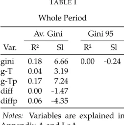
The relationships between the independent variables Gini before and after transfers

and redistribution with the dependent variable accumulated growth of GDP per capita

for the whole period are depicted in Table I. Since only for Gini after transfers data is

TABLEI

Whole Period

Av. Gini Gini 95

Var. R² Sl R² Sl

gini 0.18 6.66 0.00 −_0.24

g-T 0.04 3.19 g-Tp 0.17 7.24 diff 0.00 −_1.47

diffp 0.06 −4.35

Notes: Variables are explained in Appendix A and LoA .

of the available data in this period. The result for using the Gini values from the starting

point as the independent variable is not comparable with the other results, which use

averages, since less observations are available in 1995. For both variables Gini before

and after transfers and both specifications in the definition of including pensions or not a

positive relationship to accumulated growth is present, while redistribution seems to be

negatively but less significantly correlated with accumulated growth.

4.1.2. Long Run: 10 Year Periods

TABLEII

Relationship to Accumulated Growth for 10 Year Periods

Av. Gini Gini t Av. Gini-T Gini t - T Av. Diff. Diff. t

TS R² Sl R² Sl R² Sl R² Sl R² Sl R² Sl

95-05 0.31 3.22 0.14 2.09 0.43 4.51 0.01 −_1.04

96-06 0.37 4.32 0.09 1.28 0.38 5.18 0.05 −_2.37

97-07 0.32 4.50 0.08 0.96 0.25 4.83 0.06 −_3.14

98-08 0.23 3.53 0.06 0.56 0.09 2.72 0.12 −_3.94

99-09 0.20 2.60 0.20 1.09 0.04 1.30 0.16 −_3.57

00-10 0.16 2.39 0.26 2.70 0.04 1.27 0.12 −_3.07

01-11 0.10 2.12 0.15 2.40 0.04 1.41 0.04 −_1.99

02-12 0.08 1.93 0.14 2.44 0.02 1.22 0.03 −_1.77

03-13 0.06 1.61 0.15 2.32 0.02 1.05 0.23 −_{2.90 0.02} −_{1.34 0.48 3.46}

04-14 0.06 1.62 0.21 2.49 0.03 1.21 0.21 2.70 0.01 −_{1.04 0.01 0.64}

Notes:Variables are explained in Appendix A and LoA.

To shorten the analysis, from this point onwards pensions are excluded in the definition

of transfers. Again, the relationship between average Gini and accumulated growth is

positive and the relationship between redistribution and accumulated growth negative

for all possible periods. The positive relationship for both pre- and post-transfer Gini

tends to get weaker the more one advances in time. Results for taking the starting value

of Gini or redistribution as the independent variable should be treated with caution since

different sample sizes of countries are considered.

4.1.3. Medium Run: Five Year Periods

TABLEIII

Relationship to Accumulated Growth for Five Year Periods

Av. Gini Gini t Av. Gini-T Gini t - T Av. Diff. Diff. t

TS R² Sl R² Sl R² Sl R² Sl R² Sl R² Sl

95-00 0.05 0.55 0.03 0.58 96-01 0.25 1.22 0.03 0.42 97-02 0.31 1.36 0.09 0.51

98-03 0.31 1.50 0.21 0.63 0.38 2.08 0.00 −_0.12

99-04 0.29 1.72 0.18 0.79 0.29 2.13 0.02 −_0.58

00-05 0.26 1.82 0.25 1.79 0.26 2.08 0.07 −_1.39

01-06 0.27 2.00 0.25 1.98 0.21 2.07 0.09 −_1.73

02-07 0.23 2.00 0.26 2.16 0.14 1.86 0.09 −_1.93

03-08 0.11 1.19 0.20 1.52 0.01 0.49 0.24 −_{1.09 0.13} −_{2.07 0.19} −_0.78

04-09 0.06 0.56 0.39 0.95 0.01 −_{0.19 0.22 0.86 0.23} −_{1.58 0.14} −_0.75

05-10 0.00 0.12 0.01 0.17 0.04 −_{0.47 0.00} −_{0.12 0.12} −_{1.02 0.04} −_0.60

06-11 0.01 −_{0.19 0.00} −_{0.05 0.02} −_{0.38 0.00} −_{0.01 0.01} −_{0.27 0.00 0.10}

07-12 0.02 −_{0.36 0.03} −_{0.43 0.03} −_{0.46 0.03} −_{0.50 0.00} −_{0.16 0.00 0.10}

08-13 0.00 0.03 0.00 0.18 0.01 0.33 0.02 0.48 0.01 0.46 0.01 0.48 09-14 0.02 0.57 0.05 0.95 0.05 0.97 0.09 1.29 0.02 0.67 0.01 0.39 05-14* 0.00 0.05 0.00 0.17 0.00 0.01 0.01 0.32 0.00 −_{0.05 0.00 0.17}

Notes:Variables are explained in Appendix A and LoA. *_{All possible combinations}

In Table III the same relationships are presented as in Table II for five year periods,

or the medium run. Estimation results from regressing the starting value of Gini or

re-distribution on accumulated growth are more reliable from 2005 onwards since from this

sig-nificant in general and the relationships less strong, which makes sense, since in shorter

periods countries have less time to accumulate growth leading to less volatile results.

For the periods starting in 2006 and 2007 even a small insignificant negative relationship

between Gini and accumulated growth is observable. For pre-transfer Gini, this period

gets extended to periods starting from 2004 until 2007. Considering average

redistribu-tion, a switch in the sign from negative to positive is apparent for 2008 and 2009, while

when taking the starting level of each period for redistribution this period gets extended

to 2006 until 2009. Combining all possible observations from 2005 until 2014 all estimated

relationships turn out to be rather insignificant.

4.1.4. Short Run: Three Year Periods

TABLEIV

Relationship to Accumulated Growth for Three Year Periods

Av. Gini Gini t Av. Gini-T Gini t - T Av. Diff. Diff. t

TS R² Sl R² Sl R² Sl R² Sl R² Sl R² Sl

95-98 0.06 0.42 0.15 0.83 96-99 0.00 0.10 0.00 0.07 97-00 0.06 0.36 0.02 −_0.17

98-01 0.22 0.51 0.05 0.20 99-02 0.31 0.99 0.25 0.66

00-03 0.32 1.29 0.27 1.17 0.35 1.79 0.31 −_1.37

01-04 0.23 1.03 0.18 0.94 0.16 1.07 0.04 −_0.52

02-05 0.21 0.90 0.22 0.95 0.21 1.06 0.04 −_0.65

03-06 0.22 0.93 0.24 1.01 0.16 0.98 0.00 0.05 0.06 −_{0.81 0.01} −_0.12

04-07 0.24 1.25 0.39 1.45 0.16 1.23 0.39 1.69 0.06 −_{1.01 0.01} −_0.25

05-08 0.08 0.65 0.08 0.58 0.00 −_{0.08 0.01 0.22 0.20} −_{1.49 0.10} −_1.02

06-09 0.02 −_{0.21 0.01} −_{0.09 0.31} −_{0.81 0.15} −_{0.55 0.23} −_{0.90 0.15} −_0.74

07-10 0.13 −_{0.56 0.16} −_{0.60 0.27} −_{0.86 0.27} −_{0.88 0.04} −_{0.40 0.01} −_0.17

08-11 0.03 −_{0.31 0.03} −_{0.29 0.00 0.06 0.00 0.06 0.07 0.55 0.08 0.68}

09-12 0.00 0.21 0.02 0.42 0.04 0.58 0.06 0.73 0.02 0.59 0.01 0.42 10-13 0.02 0.44 0.07 0.85 0.04 0.60 0.10 0.89 0.01 0.35 0.01 0.34 11-14 0.02 0.36 0.05 0.52 0.04 0.45 0.08 0.61 0.00 0.17 0.01 0.26 05-14* 0.00 0.09 0.01 0.20 0.00 0.01 0.01 0.28 0.00 −_{0.12 0.00 0.10}

Notes:Variables are explained in Appendix A and LoA. *_{All possible combinations}

short run. Again, for most of the periods the relationship between Gini and accumulated

growth turns out to be slightly positive. Only for Gini after transfers in the periods

start-ing from 2006 to 2008 and for average Gini before transfers for the periods startstart-ing from

2005 to 2007 a negative relationship exists. For redistribution, a negative relationship is

apparent for all periods with starting points until 2007. From 2008 onwards the

relation-ship switches to positive. Results for all possible combinations of observations from 2005

until 2014 are again insignificant.

Because of the presence of a slight change in the sign for the Gini to accumulated

growth relationship around the years of the outbreak of the financial crisis the next

logi-cal step in the analysis is arguably to split the whole sample period into two. One, where

there is a positive relationship before the structural break and one, where there is a

neg-ative one to see how this impacts the analysis. The best attempt of doing so seems to be

the period prior to the financial crisis from 1995 to 2007 (period A) and the crisis/post

crisis period from 2007 to 2014 (period B).

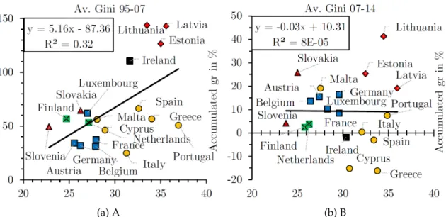
4.1.5. Two Periods

The relationship between average Gini and accumulated GDP per capita growth for

the period 1995 to 2007 is represented in Figure 3a. A strong positive relationship is

esti-mated mainly driven by the immense growth of the Baltic countries, which all have high

levels of inequality. Further, Ireland also having a high level of inequality experienced a

lot of growth in this period. Again, all countries within one regime tend to be positioned

very similar to other countries in the same regime, showing similar growth rates and

levels of inequality.

Figure 3b shows the relationship between the average Gini and accumulated GDP

per capita growth for period B from 2007 to 2014. Compared to period A the situation

re-(a) A (b) B

FIGURE3: Relationship: Gini and Accumulated Growth for Two Periods

Notes: Variables are explained in Appendix A and LoA. The black lines represent the regression lines. Regimes are distinguished by colour/symbol. The regression equations and R2are depicted in the upper left corners.

lationship turned slightly negative. Mediterranean regimes, with the exception being

Malta, performed badly showing negative growth rates for Spain, Cyprus and Greece.

Ireland, which experienced a high growth rate for period A, also shows to have a

nega-tive growth rate for period B. The Baltic countries still have high growth rates. Otherwise

the relative positioning of the involved countries is very similar as in the other

regres-sions.

TABLEV

Relationship to Accumulated Growth for Two Periods

Whole A (95-07) B (07-14)

Av. t Av. t Av. t

Var. R² Sl R² Sl R² Sl R² Sl R² Sl R² Sl

gini 0.18 6.66 0.00 −_{0.24 0.32 5.16 0.13 2.70 0.00} −_{0.03 0.00} −_0.12

g-T 0.04 3.19 0.00 0.08 0.01 0.38

g-Tp 0.17 7.24 0.00 −_{0.13 0.00} −_0.14

diff 0.00 −_{1.47 0.00} −_{0.16 0.00 0.02}

diffp 0.06 −_{4.35 0.00 0.15 0.02 0.48}

Notes:Variables are explained in Appendix A and LoA.

and the division of period A and B. For period A, only the relationship to post-transfer

Gini can be considered because of limited data availability. As stated before, this

rela-tionship is positive, while in period B all relarela-tionships are rather insignificant.

The following part of this paper deals with growth spells. The methods applied follow

closely Kourtellos & Tsangarides (2015). First some descriptive statistics of up-breaks,

down-breaks and growth spells are provided, followed by regressions on durations and

frequencies of growth spells.

4.2. Growth Spells

TABLEVI

Growth Breaks

Region Cnty Total Av. size 95-99 00s 10-14

Up 19 59 2.86 11 30 18

SD 2 6 2.17 1 3 2

CC 5 23 2.17 4 14 5

L 1 3 2.00 0 1 2

M 6 15 2.73 3 9 3

EE 5 12 4.92 3 3 6

Down 19 59 2.18 4 43 11

SD 2 7 2.71 0 5 2

CC 5 23 1.64 1 15 6

L 1 3 2.00 0 2 1

M 6 16 3.06 1 14 1

EE 5 10 1.70 2 7 1

TABLEVII

Growth Spells

Region Spells Av. dur. ≥_{10 yrs}

Complete 48 2.94 0.04

SD 6 2.17 0.00

CC 21 2.24 0.00

L 2 2.50 0.00

M 12 2.92 0.00

EE 7 5.86 0.29

Incomplete 21 3.05 0.05

SD 1 5.00 0.00

CC 3 2.67 0.00

L 2 4.00 0.00

M 7 3.71 0.00

EE 8 2.13 0.13

Combined 69 2.97 0.04

SD 7 2.57 0.00

CC 24 2.29 0.00

L 4 3.25 0.00

M 19 3.21 0.00

EE 15 3.87 0.20

Notes:Variables are explained in Appendix A and LoA.

All identified up- and down-breaks for each regime are shown in Table VI. Up-breaks

are defined as periods in which the growth rate increases from below 2% to above 2%,

up-breaks and 59 down-breaks have been identified. The average break size was similar

for most regimes. Only for eastern European countries it was substantially larger. Most

of the down-breaks occurred in the 2000s, while Mediterranean countries had the largest

average down-break size and eastern European countries the lowest.

Table VII presents duration and frequency of growth spells. Hereby, one can

distin-guish between complete and incomplete growth spells. For complete growth spells the

earlier mentioned definition applies. Incomplete growth spells refer to periods, in which

the growth spell is cut off by the time frame used, meaning periods, which had growth

rates of at least 2% but not simultaneously an up- and down-break. The only regimes,

which have growth periods of at least 10 years, are the Eastern European regimes. There

are 69 total spells in the sample, which have an average duration of close to three years

for all regimes. On average Eastern European regimes experienced the longest and social

democratic ones the shortest growth spells.

TABLEVIII

Average Before, During and After Growth Spells

(a) Growth

Region Before During After

Complete −_{0.44 4.55} −_0.61

SD −_{0.46 4.85} −_0.56

CC −_{0.30 3.93} −_0.15

L −_{1.87 4.54} −_1.25

M −_{0.09 4.66} −_0.91

EE −_{1.05 5.95} −_1.31

Incomplete −_{1.47 5.02} −_1.35

SD 0.00 6.35 0.06

CC 1.23 4.15 −3.58

L 1.72 6.20 0.49

M −_{0.15 4.27 0.08}

EE −3.99 5.54 −3.58

(b) Gini

Before During After

28.32 28.44 28.46 26.41 25.37 25.97 27.63 27.54 27.62 29.90 31.09 30.08 31.70 31.30 31.29 22.97 28.02 27.66

30.66 30.92 31.33 27.00 27.38 28.30 28.80 26.00 30.15 31.35 29.80 32.31 33.35 33.24 30.71 30.41 34.50

(c) Redistribution

Before During After

6.02 5.70 5.76

7.78 7.58 7.65

6.51 6.58 6.62

12.37 12.66 14.26

2.50 2.59 2.90

3.60 4.11 3.66

5.43 5.79 3.20

6.93 7.03

16.15 15.80

3.95 4.67

3.58 4.26 3.20

Notes:Variables are explained in Appendix A.

Table VIIIa displays the average growth rates before, during and after growth spells.

slightly negative for all regimes. For incomplete growth spells the results are much more

volatile since there is not much data on this variable. Eastern European regimes’ growth

rates turn out to be far more volatile than for other regimes, having high growth rates

on average during growths spells, while having highly negative ones before and after

growth spells.

Average inequality before, during and after growth spells is depicted in Table VIIIb.

The results must be treated with caution since data is limited for the Gini coefficient.

Nevertheless, one can see that inequality before, during and after incomplete or complete

growth spells does not vary much from scenario to scenario for the regimes involved.

Table VIIIc shows average redistribution before, during and after growth spells. Due

to the small number of observations results for incomplete growth spells must be treated

with caution. In the case of complete growth spells there are no big differences for

aver-age levels of redistribution before, during and after growth spells.

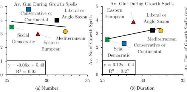
The next part summarises conducted regressions for growth spells.

(a) Number (b) Duration

FIGURE4: Relationship: Gini and Growth Spells for Regimes