UNCORRECTED PROOF
Thin-Walled Structures](]]]])]]]–]]]
Numerical analysis of piping elbows for in-plane bending and internal
pressure
E.M.M. Fonseca
a,, F.J.M.Q. de Melo
b, C.A.M. Oliveira
caDepartment of Applied Mechanics, Polytechnic Institute of Braganc
-a, Portugal bDepartment of Mechanical Engineering, University of Aveiro, Portugal c
Department of Mechanical Engineering, Faculty of Engineering of University of Porto, Portugal Received 27 October 2005; accepted 12 April 2006
Abstract
This work presents the development of two different finite piping elbow elements with two nodal tubular sections for mechanical analysis. The formulation is based on thin shell displacement theory, where the displacement is based on high-order polynomial or trigonometric functions for rigid-beam displacement, and uses Fourier series to model warping and ovalization phenomena of cross-tubular section. To model the internal pressure effect an additional formulation is used in the elementary stiffness matrix definition. Elbows attached to nozzle or straight pipes produce a stiffening effect due to the restraint of ovalization provided by the adjacent components. When submitted to any efforts, the excessive oval shape may reduce the structural resistance and can lead to structural collapse. For design tubular systems it is also important to consider the internal-pressure effect, given its effect on the reduction of the pipe flexibility. Some conclusions and examples are compared with results produced by other authors.
r2006 Published by Elsevier Ltd.
Keywords:Finite piping elbow element; Flexibility; Tubular section; In-plane bending; Internal pressure
0. Introduction
The main objective of this investigation has focused on the development of a computational model for the analysis of the stiffness piping elbows under any type of mechanical loading. Piping systems are constituted by straight and curved elements and exhibit complex deformations given their toroidal geometry and the multiplicity of the loading conditions. Several authors have studied the bending stiffness of curved thin-walled pipes: von Ka´rma´n [1]
solved the problem using the Rayleigh–Ritz method, O¨ry and Wilczek[2]presented a economical method which uses a transfer matrix to able stress and deformation calcula-tion, Thomson [3]worked with an analytical formulation using a development with trigonometric series functions
and realized many experimental studies, Thomas [4]
studied the stiffening effect on thin-walled piping elbows using a thin-shell element from a finite-difference program,
more recently Bathe and Almeida [5] formulated a pipe
elbow element using a cubic displacement interpolation based on finite-element method with ovalization phenom-ena contribution. In this paper an alternative formulation is presented for the characterization of the deformation of thin-walled piping elbow element, based on shell displace-ment field and on additional formulation to obtain the elementary stiffness matrix due to internal pressure. A finite element with two nodes was developed, where the displacement field is based on high-order polynomial functions for rigid beam displacement, such as the equations developed by Fonseca et al. [6]or a new model proposed here with trigonometric functions and the development of Fourier series to model warping and ovalization of tubular section, reported in [3]. The two different computational models presented in this work have been tested with some numerical examples and experi-mental measurements obtained by other authors.
www.elsevier.com/locate/tws 1
3
5
7
9
11
13
15
17
19
21
23
25
27
29
31
33
35
37
39
41
43
45
47
49
51
53
55
57
59
61
63
65
67
69
71
73
75
77
79
81 0263-8231/$ - see front matterr2006 Published by Elsevier Ltd.
doi:10.1016/j.tws.2006.04.005
Corresponding author. Fax: +351 273 313 051.
UNCORRECTED PROOF
1. Essential assumptions
The geometric parameters considered for the piping elbow element definition are: the arc length s, the mean curvature radiusR, the thicknessh, the mean section radius of the pipe r and the central angle a. Fig. 1 presents the geometric parameters defining the two nodal tubular sections.
The deformation field of a piping elbow element refers to membrane strains and shell curvature variations. The following assumptions, referred to in[6–9], were considered in the present analysis: the curvature radius is assumed much larger than the section radius; a semi-membrane deformation model is adopted and it neglects the bending stiffness along the longitudinal direction of the toroidal shell but considers the meridional bending resulting from ovalization. The shell is considered thin and inextensible along the meridional direction for only the mechanical loading case.
2. Finite piping elbow element formulation
The shell finite-element displacement field resulting from the superposition of rigid-beam displacement and the complete Fourier expansion for ovalization and warping terms are as shown in the following equations:
u¼Uð Þs rcosy jð Þs þu s;ð yÞ, (1a)
v¼ Wð Þs sinyþv s;ð yÞ, (1b)
w¼Wð Þs cosyþw s;ð yÞ, (1c)
wherew(s,y) is the surface displacement in radial direction resulting from ovalization, v(s,y) the meridional displace-ment due to ovalization, u(s,y) the longitudinal
displace-ment due to warping tubular section effect, U the
tangential beam displacement, W the transversal beam
displacement and j represents the beam rotation in z
direction.
The displacements u, v and w are calculated on shell surface from the finite piping elbow element (Fig. 1), as a function of a displacement field under mean line arc (U,W
and j) as shown Fig. 2. Those parameters are related
through simple differential equations from beam-bending theory.
Two different models will be presented for the displace-ment field calculation in piping elbow eledisplace-ments. In the first model, a high-order formulation should be used and six parameters are necessary to define the beam displacement
field. From this, U can be approached by the following
fifth-order polynomial (5P):
UðsÞ¼aoþa1sþa2s2þa3s3þa4s4þa5s5. (2a)
The transverse displacement and the rotation can be calculated as
Wð Þs ¼ R
dU
ds ¼ R a1þ2a2sþ3a3s 2
þ4a4s3þ5a5s4
,
(2b)
jð Þs ¼dW
ds ¼ R 2a2þ6a3sþ12a4s 2
þ20a5s3
. (2c)
The coefficients are determined as a function of imposed boundary conditions under the curved referential.
The second model is a formulation based on trigono-metric functions (TF) and four parameters are necessary to define the beam displacement field.Ucan be approximated by the following function:
UðsÞ¼b1 cos
s R
þb2sin s R
þb3 cos 2 s R
þb4 sin 2 s R
.
(3a)
The transverse displacement can be calculated as
WðsÞ¼ R
dU
ds ¼b1 sin s R
b2 cos s R
þ2b3 sin 2 s R
2b4 cos 2 s R
. ð3bÞ
For the rotation field a linear polynomial may be used:
jð Þs ¼b5þb6S. (3c)
The coefficients are determined using the same imposed boundary conditions under the curved referential. For straight-pipe elements a formulation based on third-order polynomial (3P) was used with Hermitian shape functions. The surface displacements in radial and in meridional directions result from ovalization, in-plane, as discussed by Thomson[3]and are given by the following equations:
w s;ð yÞ ¼ X
n2
an cosny
!
Niþ
X
n2
an cosny
!
Nj, (4)
1
3
5
7
9
11
13
15
17
19
21
23
25
27
29
31
33
35
37
39
41
43
45
47
49
51
53
55
57
59
61
63
65
67
69
71
73
75
77
79
81
83
85
87
89
91
93
95
97
99
101
103
105
107
109
111
113 Fig. 1. Geometric parameters of finite piping elbow element.
UNCORRECTED PROOF
v s;ð yÞ ¼ X
n2
an
n sinny
!
Niþ
X
n2
an
n sinny
!
Nj. (5)
The longitudinal displacement due to warping tubular section effect is calculated by the following equation, discussed by Thomson[3]:
u s;ð yÞ ¼ X
n2
bn cosny
!
Niþ
X
n2
bn cosny
!
Nj. (6)
The terms anand bnare constants to be determined as function of developed Fourier series.
The mechanical deformation model considers that pipe undergoes a semi-membrane strain field, discussed[8–10], and is given by.
ess
gsy
wyy 8 > < > : 9 > = > ; ¼ q qs siny R cosy R 1 r q qy q
qs 0
0 1
r2 q qy 1 r2 q2
qy2 2 6 6 6 6 6 6 6 4 3 7 7 7 7 7 7 7 5 u v w 8 > < > : 9 > = > ; , (7)
whereessis the longitudinal membrane strain,gsythe shear strain andwyythe meridional curvature form ovalization.
The application of the virtual-work principle gives finally the system of algebraic equations to be solved. The matrix force–displacement equation for this finite-element pipe is
K
½ f g ¼d f gF . (8)
d is a nodal unknown displacement vector and F the
applied nodal forces. The element stiffness matrix K is calculated from the matrix equation
Kglobal¼½ T
Z
s
B
½ T½ D½ BdS
T
½ T, (9)
where dS¼rdsdy, T is the transpose matrix for global system,Bresults from the derivative of the shape functions for the finite piping elbow element and the elasticity matrix Dappears with a simple algebraic definition, dependent on the elastic modulus, the piping elbow thickness and Poisson’s ratio.
In the piping elbow element formulation, a Gaussian integration was carried out along variableswhile an exact one was used along the circumferential direction y. In detail, the stiffness terms resulting from the beam shear deformation were calculated using one-point gauss inte-gration when a reduced inteinte-gration (for TF polynomial) and a complete integration for (5P and 3P polynomials) are used, while all the remaining stiffness terms were calculated with two-point gauss integration (ovalization and warping terms). Due to the uncoupled formulation of the displace-mentWand the section rotationjin the TF element, it is necessary that a different type of integration should be used along variables. This expedient avoids the element locking, a numerical drawback associated with the contribution shear terms in the stiffness matrix when exact integrations are used. The use of selective reduced integration only for
shear terms has shown a remarkable improvement in the numerical behaviour of pipe elements, a procedure used by Melo and Castro[8]and Prathap[11].
The total number of degrees of freedom for this element is 2(3+2Ny), where Ny is the number of terms used in Fourier expansions (8 terms).
3. Influence of internal pressure in stiffness matrix determination
To consider the effect of the internal pressure in the tubular system an infinitesimal pipe area is defined, accounting for the work produced by the pressure load in the pure bending of the piping elbow, as in[5]. Considering the tubular section inextensible, the piping-elbow length is the same but there is a volume variation produced by an increase of pipe deformation work, due to internal pressure. The deformation work is calculated as
Welbow¼pDV¼
Z L
0 Z 2p
0
pðRrcosyÞa
2 dA s;ð yÞ, (10)
Wstraigth¼pDV¼
Z L
0 Z 2p
0 p
2LdA s;ð yÞ, (11)
where p represents the internal pressure, (Rcosy)a or L the arc length for the mean piping-elbow surface, s the longitudinal coordinate and dA(s,y) the modified tubular section area.
Considering a differential element area before and after ovalization,Fig. 3, the following expression may be used to calculate dA(s,y).
In Fig. 3the arc element length AB is equal to the arc element length A0B0, considering the inextensible condition. The infinitesimal area ABA0B0, is given by the following equation, neglecting the second-order quantities and dv¼ wdy (pipe inextensible):
UNCORRECTED PROOF
dA s;ð yÞ ¼1
2ðrþwÞðrþwÞdy 1 2rrdy
1
2ðrþwÞdydw
þwv
2
1
2ðvþdvÞðwdwÞ
ffiw2dyþ1
2vdwþwrdy¼w 2dy
þwrdy
þ12vdw
dy dy ð12Þ
If internal pressure is considered as a dominant factor into piping elbow ovalization,w andvrepresents the displace-ments by Eqs. (4) and (5), respectively.
Substituting the expressions and considering the internal product of wwith rdy equals zero, the deformation work for tubular curved and straight pipes may be calculated:
Welbow¼
3 4paRpa
2
i or Wstraight¼
3 4ppLa
2
i. (13)
Results from these equations must be added to the diagonal terms of elementary stiffness matrix, Eq. (9), referred to as ovalization terms.
4. Study case: Flexibility factor for in-plane bending with internal pressure effect
Fig. 4represents an half of a tubular structure reported in Ref. [5]. One-dimensional mesh was used with straight and curved elements considering the two different models presented (5P+3P and TF+3P). It was applied a vertical load at an extremity of the structural piping system and different values of internal pressure were used. The elbow
factorh¼hR= r2 ffiffiffiffiffiffiffiffiffiffiffiffiffi
1n2 p
¼0:1084.
Fig. 5 represents the calculated flexibility factor k¼ 4Er3tj
ðnode6Þ=MR 1n2
for the piping-elbow system using our two different models and results reported in Ref.[5]. It was shown the internal pressure has influence on the global stiffness of the structure. The main effect of the internal pressure consists in decreasing of the piping-elbow flexibility.
5. Study case: Flexibility coefficient determination in different types of piping elbows and nozzle constraints
Fig. 6 show the geometry created for in-plane bending and with internal-pressure effect. This figure represents also the one-dimensional mesh used for each model. The
bending moment is equal M¼73450 Nm and in the
internal pressure considered is equal P¼100 MPa.The
pipe material has an elasticity modulus equal to 210 GPa. For simulating the stiffening effect of a nozzle, a different length of constraintXis considered as well as a built-in-end extremity. The numerical results obtained with our two different formulations (5P+3P and TF+3P) for different imposed loadings (bending moment or a bending moment and internal pressure) are compared with solution pre-1
3
5
7
9
11
13
15
17
19
21
23
25
27
29
31
33
35
37
39
41
43
45
47
49
51
53
55
57
59
61
63
65
67
69
71
73
75
77
79
81
83
85
87
89
91
93
95
97
99
101
103
105
107
109
111
113 P
h=0.5 in r=14.75 in
45
°
R=45 in L=59 in.
1
2
3
4
5
6 7
8 9
10 11
12 13
14 15 16 Y
X Z
Fig. 4. Piping elbow geometry and loading. One-dimensional mesh used.
0 2 4 6 8 10 12 14 16
0 200 400 600 800 1000 1200
Pressão [Psi]
Flexibility factor k
ADINAP ref [7] Exper. ref [7]
(5P+3P) (TF+3P)
UNCORRECTED PROOF
sented by Thomas[4], when considering the elbow factor
h¼hR
r2¼0:1304.
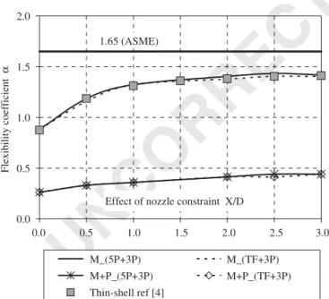
The curves shown inFig. 7represent the elbow bending flexibility coefficient a¼2Ert2j
ðnode13Þ=M, using equation
k¼a=h, which is affected by the presence of nozzle
constraint and is obtained with different loading types. As seen when the internal pressure is added, the structural stiffness increases. According to the ASME Designing Code, the calculation of the flexibility factorkin the curved pipe under uniform bending and unflanged bends is determined using k¼1:65=h, represented inFig. 8.
It was shown the elbow with a rigid flange at one end and a pipe on the other is about twice as stiff as an isolated elbow. The presence of a rigid restraint near one end of the elbow shifts the maximum ovalization from the mid-span of the elbow. These conclusions are in good agreement with the observations of Thomas, when finite thin-shell elements are used.
Fig. 8 presents the ovalization problem obtained with our numerical results calculated at the surface tubular section, for any differentXlength, at the transverse-section elbow at mid-span for each loading situation.
6. Conclusions
Results of flexibility coefficient from mechanical actions, including internal pressure, was presented with two 1
3
5
7
9
11
13
15
17
19
21
23
25
27
29
31
33
35
37
39
41
43
45
47
49
51
53
55
57
59
61
63
65
67
69
71
73
75
77
79
81
83
85
87
89
91
93
95
97
99
101
103
105
107
109
111
113 Fig. 6. Piping elbows geometry and loading conditions used. One-dimensional mesh used.
0.0 0.5 1.0 1.5 2.0
0.0 0.5 1.0 1.5 2.0 2.5 3.0 Effect of nozzle constraint X/D
Flexibility coefficient
α
M_(5P+3P) M_(TF+3P)
M+P_(5P+3P) M+P_(TF+3P) Thin-shell ref [4]
1.65 (ASME)
UNCORRECTED PROOF
different formulations. With these new finite piping elbow elements it is possible to calculate the displacement field due to any type of load for in-plane loading. It is a simple finite element and easy to operate and avoids a pre-processing expensive mesh generation for shell definition surface. The purpose of this paper is to provide an easy and an alternative formulation when compared with a complex finite shell, solid or beam element analysis for the same application. Several case studies presented were compared with results reported by other authors and discussed.
References
[1] von Ka´rma´n Th. Die Forma¨nderung du¨nnwandiger Rohre. Insbe-sondere federnder Ausgleichsrohre, Zeitschrift des Vereins deutscher Ingenieure, 1911.
[2] O¨ry H, Wilczek E. Stress and stiffness calculation of thin-walled curved pipes with realistic boundary conditions being loaded in the plane of curvature. Int J Pressure Vessels Piping 1983;12:167–89. [3] Thomson G. The influence of end constraints on pipe bends. PhD
Thesis, University of Strathclyde, Scotland, 1980.
[4] Thomas K. Stiffening effects on thin-walled piping elbows of adjacent piping and nozzle constraints. Pressure Vessels Piping Div ASME 1981;50:93–108.
[5] Bathe KJ, Almeida CA. A simple and effective pipe elbow element. Pressure stiffening effects. J Appl Mech 1982;49:914–6.
[6] Fonseca EMM, Melo FJMQ, Oliveira CAM. The thermal and mechanical behaviour of structural steel piping systems. Int J Pressure Vessels Piping 2005;82(2):145–53.
[7] Fonseca EMM, Melo FJMQ, Oliveira CAM. Determination of flexibility factors on curved pipes with end restraints using a semi-analytic formulation. Int J Pressure Vessels and Piping 2002;79(12):829–40.
[8] Melo FJMQ, Castro PMST. A reduced integration Mindlin beam element for linear elastic stress analysis of curved pipes under generalized in-plane loading. Comput Struct 1992;43(4):787–94. [9] Flu¨gge W. Thin elastic shells. Berlin: Springer; 1973.
[10] Kitching R. Smooth and mitred pipe bends. In: Gill SS, editor. The stress analysis of pressure vessels and pressure vessels components. Oxford: Pergamon Press; 1970 [Chapter 7].
[11] Prathap G. The curved beam/deep arch/finite ring element revisited. Int J Num Meth Eng 1985;21(3):389–407.
1
3
5
7
9
11
13
15
17
19
21
23
25
27
29
31
33
35
37
39
41
43
45
47
49
51
53
55
57
59
61
63
65
67
69
71
73
75
77
79
81
83
85
87
89
91 90°
0°
180°
270° Moment
indeformable section
>>X
90° 0°
180°
270° Moment+Pressure indeformable section
>>X

![Fig. 4 represents an half of a tubular structure reported in Ref. [5]. One-dimensional mesh was used with straight and curved elements considering the two different models presented (5P+3P and TF+3P)](https://thumb-eu.123doks.com/thumbv2/123dok_br/16862838.753775/4.892.40.826.102.798/represents-structure-reported-dimensional-straight-considering-different-presented.webp)