V ELMA DEJ ESUSR ODRIGUES

(1)

M

ASTER IN

FINANCE

M

ASTER

’

S

F

INAL

W

ORK

P

ROJECT WORK

F

ITTING THE

T

ERM

S

TRUCTURE OF YIELD SPREADS

V

ELMA DE

J

ESUS

R

ODRIGUES

(2)

M

ASTER IN

FINANCE

M

ASTER

’

S

F

INAL

W

ORK

P

ROJECT WORK

F

ITTING

T

HE

T

ERM

S

TRUCTURE OF

Y

IELD

S

PREADS

V

ELMA DE

J

ESUS

R

ODRIGUES

S

UPERVISOR

:

P

ROFESSOR

D

OCTOR

R

AQUEL

M

EDEIROS

G

ASPAR

C

O

-S

UPERVISOR

:

D

OCTOR

P

EDRO

B

ALTAZAR

(3)

Abstract

This study aims to fit and analyze the behavior of the Yield Spread curve in the

context of Portugal Government Bonds, covering a period of January 2004 through

June 2014, when Portugal faced a liquidity and debt crisis. In order to extract

the Yield Spread curve, we use a disjoint method. This method requires as an

in-put both a defaultable and non-defaultable term structure: we use the default-free

curve estimated by the ECB and the defaultable term structure is estimated by

the Nelson-Siegel model (1987). Due to the important role that forecasting plays

in understanding how term structure evolves, the secondary objective of this work

is to forecast the yield curve by predicting the parameters of Nelson-Siegel model

(1987) using the Random Walk with drift as the benchmark model and the AR(1)

and the VAR(1) model as competitors models. The results include the empirical

analysis of Portuguese Government yield spread curve and, concerning the yield

curve forecasting, we conclude that AR(1) and VAR(1) slightly outperformed the

benchmark model and these models performance improves as the forecasting time

horizon increases.

Keywords: Yield Curve, Yield Spread, Nelson-Siegel Model, Forecasting, Term

(4)

List of Abbreviations

ACT/ACT- Actual/Actual convention

AIC -Akaike’s Information Criterion

AR(1)- Autoregressive Process of Order 1

BIC - Bayesian Information Criterion

ECB - European Central Bank

EMU- Economic Monetary Union

ICMA - International Capital Market Association

ISIN- International Securities Identification Number

OLS - Ordinary Least Squares

GLS - Generalized Least Squares

RW- Random walk

VAR(1)- Vector Autoregressive Process of Order 1

List of Tables

1 Regressions estimated for Random Walk with Drift . . . 26

2 Regressions estimated for AR(1) . . . 27

3 Regressions estimated for VAR(1) . . . 28

A1 Descriptive Statistics of Portuguese Government Bonds Yield Curve.The

(5)

A2 Descriptive Statistics of Estimated Parameters, sample period: 2004:01

to 2014:06. . . 35

A3 Descriptive Statistics Portuguese Government Bonds of Yield Spread. Sample Period: 2004:01 to 2014:06. . . 36

A4 Out-of-sample Forecasting Results, RW with drift: 1-month ahead . . 37

A7 Out-of-sample Forecasting Results, AR(1): 1-month ahead . . . 38

A10 Out-of-sample Forecasting Results, VAR(1): 1-month ahead . . . 39

A13 Forecasting Model Selection Criteria computed for the RW with drift, AR(1) and VAR(1). . . 40

List of Figures

1 Selected Fitted Yield Curve . . . 18

2 Selected Fitted Yield Curve (Continuation) . . . 19

(6)

4 Portuguese Government Bonds Yield Spread over the period January

2004 through June 2014 . . . 21

5 Impact of financial bailout on the yield curve . . . 24

A1 Portuguese Treasury Bonds Yield Curve daily fit of year 2006. . . 41

A2 Portuguese Government Bonds Yield Curve daily fit of year 2011. . . 41

A5 Pricing errors generated by estimating the yield curve over the period

January 1st _{2004 through June 30}th _{2014. . . 43}

A6 Yield errors generated by estimating the yield curve over the period

(7)

1 Introduction

In the recent past, the financial industry as a whole has changed rapidly. The rapid

development of government bond markets in Euro-zone may be explained by the

ef-fects of globalization and the process of European Monetary integration. Although

the creation of European Monetary Union theoretically eliminates the exchange rate

risk, yield spread still exists due to liquidity issues and country-specific default risk

explained by the adoption of a certain fiscal policy and external shocks. So,

un-derstanding the evolution of yield spread is a crucial subject in finance, since the

historical spreads may give to investors an overview about market expectations,

po-tential investment opportunities or how to hedge portfolios. A proper yield spread

evolution assessment will bring value to fixed income managers and, since the yield

spread is a source of risk, it must be considered in financial risk management,

pric-ing financial products, fiscal debt, portfolio allocation, or even in monetary policy

implementation.

Given the importance of this topic, there are several empirical literature that

focus on the time-series dynamics of yield spread. Duffee (1999) and Elton et al.

(2001) both fitted the credit spread using non-callable corporate bonds. The

em-pirical research of Elton et al. (2001) investigates the existence of risk premium

in corporate bonds spread and they conclude that the credit spread may be

ex-plained by the expected default loss, tax premium and risk premium. Since a large

part of existence empirical research on fitting the yield spread of corporate bond

(9)

1 INTRODUCTION

of callable corporate bonds by treating simultaneously the effect of credit risk and

optionality. There are also empirical studies based on the extraction of

Govern-ment yield spread, such as, Dullman and Windfuhr (2000), Geyer et al. (2003) and

Duffie et al. (2003). The research of Dullman and Windfuhr (2000) investigates

the dynamics of the yield spread between Italian and German Government bonds

after the exchange-rate agreement in 1998. Geyer et al. (2003) deducted the yield

spread of Government bonds issued by member states of EMU and they noted a

significant and volatile credit spread between German Bund yields and the others

member states of EMU yields. Duffie et al. (2003) developed a model, under the

framework of Duffie and Singleton (1999), that estimate the term structure of credit

spread using the Russian dollar-denominated bonds, which takes into consideration

the risks of default, risk of restructuring and compensation for lack of liquidity.

Regarding the term structure modeling, there are also a vast literature concerning

this field. The most used approach among the financial market practitioners and

central banks is the class of Nelson-Siegel Models (1987), which is used to fit the

term structure of interest rates through a flexible and smooth parametric function.

In order to increase flexibility in the standard Nelson-Siegel model (1987), Svensson

(1994) proposed to add a second hump-shape factor with its own decay parameter.

However, a multicolinearity problem may arise by adding a second decay parameter.

To overcome the multicolinearity issue Pooter (2007) proposed an Adjusted Svensson

model. Note that the original Nelson-Siegel model is a static model, which fits the

cross section of interest rates at a given point in time. That is why Diebold and Li

(10)

1 INTRODUCTION

Despite the progress in the term structure of interest rate modeling, the

practi-cal estimation of yield spread field using Portugal empiripracti-cal data has been

under-explored. This study tries to fill this gap by fitting the yield spread curve in the

context of Portuguese Government Bonds. The latter yield spread curve is computed

as the difference of Portuguese Yield Curve, which is estimated using the standard

Nelson-Siegel model (1987), and the yield curve of AAA-rated countries in euro area

estimated by ECB, which is considered as the benchmark zero-coupon yield curve.

Since this research covers the period that Portugal was under the Economic and

Financial Adjustment Programme, besides the yield spread curve behavior analysis,

is also addressed the impact of the financial bailout.

Much of this research focuses on fitting the Portuguese Treasury Bonds yield

curve and consequently the extraction of its yield spread. However, many tasks

such as pricing financial instruments, portfolio diversification or risk management,

require not only the term structure of interest rates but also the knowledge of how

the term structure will evolve plays an important role in finance. So, the secondary

aim of this research is to better understand the dynamic evolution of the yield curve.

To meet the latter objective, is performed the forecasting of the yield curve using

three different models: Random Walk with drift, AR(1) and VAR(1).

The remaining of the text is organized as follows. Section two provides a brief

discussion of the theoretical framework, where some basic concepts are highlighted.

Section 3 presents the methodology used to fit the term structure of yield spread

as well as the data chosen to achieve this purpose. Section 4 analyses the empirical

(11)

2 THEORETICAL FRAMEWORK

of this study.

2 Theoretical Framework

Here is introduced some basic concepts prior to discussing in detail the term

struc-ture model used to generate the yield curve in this research. Afterwards, is explained

the approach used to extract the yield spread curve as well as different models used

in the yield curve forecasting.

2.1 Term Structure: Basic Concepts

The term structure of interest rate depicts a series of interest rates as a function of

time to maturity. Further, there are three equivalent theoretical representation of

term structure: yield curve, forward curve and discount curve. As the latter curves

names suggest, they graphically depict a series of yields, forward rates and discount

factors as a function of maturity, respectively.

Regarding the yield curve, yt(τ), it can be computed as an equally-weighted

average of instantaneous forward rates. This sort of rate is defined as forward rate,

f_t(τ), with the limit of maturity tending to zero. More precisely, it can be interpreted

as a forward rate marginal cost for a very short period of time. So, the yield curve

or spot rate curve, withτ periods to maturity, is given by:

yt(τ) =

1

τ

Z τ

0

(12)

2.1 Term Structure: Basic Concepts 2 THEORETICAL FRAMEWORK

This important relationship between yield and forward rate is a critical point of the

Nelson-Siegel class of model.

The discount curve,Pt(τ), as mentioned before, is a function that depicts the

re-lationship between the discount factors and term to maturity and it can be obtained

from the yield curve by the following relation:

Pt(τ) = exp[−τ yt(τ)] (2)

Therefore given the relations mentioned above, we can find the following link

be-tween these three curves:

f_t(τ) =− 1

Pt(τ)

dPt(τ)

dτ =yt(τ) +τ dyt(τ)

dτ (3)

Once the yield curve or the forward curve is known, any coupon bearing bond can

be priced as a sum of discounted cash flows. Though, the three term structures

representation mentioned before are not directly observed in the market for an

ex-tensive range of maturities. Saying so, these curves must be estimated from bond

prices observed in the market using theoretical models to fit the term structure, such

as the Bootstrapping of Fama and Bliss (1987), cubic spline function of McCulloch

(1975), exponential splines of Vasicek and Fong (1982), parametric function

sug-gested by Nelson-Siegel (1987), and later extended by Svensson (1994), Bjork and

Christensen (1999), Pooter (2007) or non-parametric model introduced by Linton

et al. (2001). There are several studies that empirically compare these different

(13)

2.2 Nelson-Siegel Model (1987) 2 THEORETICAL FRAMEWORK

2.2 Nelson-Siegel Model (1987)

Nelson and Siegel (1987) proposed a three parameter exponential-polynomial

func-tion. This approach fits the forward curve with:

f_t(τ) = β0,t+β1,texp

−τ

λt

+β2,t

τ λt exp −τ λt (4)

This expression can be viewed as a constant plus a Laguerre function, which is a

product between a polynomial and an exponential decay term.

As described in the previous subsection, the yield curve is obtained by an

equally-weighted average of instantaneous forward rates. So the spot yield curve is given

by:

yt(τ) =β0,t+β1,t

   

1−exp −τ λt τ λt    

+β2,t

   

1−exp −τ λt τ λt −exp −τ λt     (5)

Thus, the shape of the yield curve is given by the sum of three components, each of

them resulting from the product of weighting functions and the model parameters

β0,t, β1,t and β2,t. Each component can be interpreted as follows. The component

β0 is multiplied by one for all maturities, so it can be interpreted as a long-term

component. The component of β1 is the short-term component, since its weighting

function starts at 1 and afterwards will decay rapidly to zero. Lastly, in the

com-ponent ofβ2, the weighting function starts at zero, increases for medium maturities

and then decays to zero again, which produce a hump-shaped curve. Moreover,

yields converge to β0 if maturity tends to infinity and converge to the sum of β0

and β1 if maturity tends to be an infinitely short period of time. Thus, β0+β1 can

(14)

2.3 Modeling the Yield Spread 2 THEORETICAL FRAMEWORK

β0 +β1 must be positive. Note that the λt parameter determines the rate of decay

and also at which maturity the medium-term component reaches its maximum.

The basic parametric model of Nelson-Siegel (1987) is a static approach, which

gives an estimation of yield curve at a certain point in time. However, Diebold and

Li (2006) suggest a dynamic version of Nelson-Siegel, where the dynamics factors

β0,β1 and β2 can be viewed as level, slope and curvature of yield curve, respectively.

Besides that, in the new dynamic framework they propose to fix the decay parameter

λ at a pre-specified value in order to ease the estimation process. More precisely, if

λ is fixed, the nonlinear measurement equations become linear and the estimation

proceed using the cross-sectional OLS procedure.

It is also worth noting that Nelson-Siegel model has enough flexibility to capture

a range of shapes of yield curve observed in the market (such as monotonic, humped

and S-shaped curve) and its dynamic version is able to replicate the stylized facts

of yield curves such as: yield curve are normally upward sloping, when yields reach

high (low) levels tend to decrease (increase) in the next moment -behavior of mean

reversion, shorter term yields are more volatile than the longer term yields,

long-term yields are more persistent than the shorter long-term.

2.3 Modeling the Yield Spread

With respect to the literature about the yield spread modeling, there are two

dif-ferent parametric models: disjoint and joint method.

Regarding the disjoint method, the basic idea is deriving both the term structure

(15)

2.3 Modeling the Yield Spread 2 THEORETICAL FRAMEWORK

separately. Thus, the term structure of zero-coupon yield spread is obtained by

the difference between the risky coupon yield curve and the benchmark

zero-coupon yield curve. In short, it is a three-step procedure. Dullman et Windfuhr

(2000) empirically computed the yield spread between German and Italian Sovereign

Bonds as the difference between the yields of Italian and German bonds. Annaert

(2000) and Landschoot (2004) both modeled the European credit spread as the

difference between the yield of the corporate bond and the yield of government

bond. However, Annaert (2000) made this subtraction with respect to the bonds

with same average duration and Landschoot (2004) divided the term structure of

yield spread by rating categories. Elton et al. (2001) empirically computed the yield

spread curve as the difference between the yield of the zero-coupon corporate bond

and the yield of zero-coupon government bond of the same maturity.

The joint estimation framework, proposed by Houweling et al. (2001), consists in

jointly estimating both term structure of zero-coupon yields simultaneously. In other

words, since a defaultable term-structure comprises in a default-free curve (proxied

by a theoretically riskless government curve) and in a yield spread curve, the basic

idea of this approach is a decomposition of the defaultable term structure into these

two features. By saying so, this method focuses in modeling the spread and the

default-free is considered as a part from the government curve. In short, all the

parameters in the model for the discount spread function and the government curve

are simultaneously estimated from a combination of both data set and performing

(16)

2.4 Forecasting the Yield Curve 2 THEORETICAL FRAMEWORK

2.4 Forecasting the Yield Curve

Modeling the yield curve is an important field in financial economics, so the

fore-casting. Many tasks such as pricing financial instruments, portfolios allocation,

managing financial risks require not only the current term structure of interest rates

but also the understanding how the yield curve may evolve. The results of the

forecast also may serve as a guideline for strategic plans concerning the fiscal debt

structuring and monetary policy.

In the context of the Nelson-Siegel model, time series models can fit to the

history of β parameters and used to forecasts. To accomplish the latter aim, the

out-of-sample forecasting will be performed using three different models: Random

Walk with drift, AR(1) and VAR(1).

The Random Walk is the simplest model. It is defined as a process where the

future value is given by the previous value plus an error. The error term is defined

as a white noise process, which is formed by a sequence of uncorrelated variables

with zero mean and constant variance. This process has the following form:

yt(τi) =yt−1(τi) +εt(τi), εt(τi)∼N(0, σ2(τi)) (6)

and it implies that all the expected future values ofYt+δ,δ >0, is given by Yt.

Whenever the time series present an average upward or downward trend, it is

expected that the forecasted values continue to exhibit a trend. In this case, a

non-zero constant trend is added to the random walk and the process is represent as

follows:

(17)

Note that forα >0 the time series will exhibit an upward trend and, consequently,

α <0 will denote a downward trend.

The random walk with drift process is particularly relevant since many financial

time series seem to follow a pattern that exhibits a trend.

The AR(1) is an univariate autoregressive model of first order and is represented

as follows:

yt(τi) =θ(τi) +φ(τi)yt−1(τi) +εt(τi), εt(τi)∼N(0, σ

2₍_τ

i)) (8)

Actually, it is a linear regression model, which the forecasted value depends on its

own past values. In this case, since there is only one lag in the autoregressive process,

the expected future value is given by the previous value plus the θ(τi). The value

of φ defines whether the time series is stationary or not. If |φ| >1, the process is

non-stationary and it grows exponentially. If|φ|<1, the process is stationary. Once

again, the error term is formed by a series of random shocks and it is uncorrelated

with the past values of the AR series. Note that whenφ(τi) takes the value of 1 this

becomes a random walk process.

The VAR(1) is a vector autoregressive process of first order, which may be used

to forecast multivariate time series. This process is given by:

yt=µ+ ΓFt−1+εt, εt∼N(0,Σ) (9)

Where Ft−1 represents the factor matrix.

The VAR(1) assumes that theεtare uncorrelated through time and independent

and identically distributed.

(18)

parameter of the Nelson-Siegel (1987) model is regressed against its own past values.

In the other hand, in VAR(1) is created a matrix where each parameter forecasted

is regressed against its own past values and against all other parameters included in

the system.

Regarding the empirical research of this field, there are several authors that

in-vestigated the quality of forecasting models based on Nelson Siegel model (1987).

Diebold and Li (2006) used several forecasting model such as Random Walk, Slope

Regression, Fama-Bliss forward rate regression, Cochrane-Piazzesi (2002) forward

curve regression, AR(1) and VAR(1) on yield levels and VAR(1) on yield changes.

By assessing the quality of the forecast based on dynamic version of Nelson-Siegel,

Diebold and Li (2006) argued that their forecasting approach produced accurate

re-sults, outperforming several benchmark forecasting model, especially for a 6 and

12-months forecast horizon. Pooter (2007) used the benchmark Random Walk model,

AR(1) and VAR(1) and the empirical results suggest that the four-factor model,

which is the model that adds a second slope to the Nelson-Siegel model, produces

forecast that outperform the benchmark Random Walk. Molenaars et al (2003)

re-sults suggest that the forecasting models used, which are the AR(1) and dynamic

Nelson-Siegel model, underperform the random walk model. Further, there is no

(19)

3 DATA AND METHODOLOGY

3 Data and Methodology

In this section is provided a detailed discussion regarding the data used in this

re-search as well as the procedure followed to fit the term structure of yield spread.

Hereafter, will be explained how the forecasting is performed.

3.1 Data Description

This research uses daily prices of Government bonds of varying maturities issued by

Portugal over the period January 1st _{2004 through June 30}th _{2014, providing ten}

years and six months of daily data, taken from Bloomberg database. Besides daily

bonds prices, the data set includes for each bond considered the issue date, maturity

date, ISIN, first coupon payment date, coupon rate, date count convention and the

amount issued.

In order to avoid distortions in the estimation, several filters are considered to

determine the sample of bonds. Similar to Diebold and Li (2006), we exclude bonds

with liquidity issues, which are Treasury Bills with less than one month to maturity

and bonds with less than one year to maturity, bonds with option features and

perpetual bonds are excluded as well.These filters, which are also applied by the

Center for Research in Security Prices, leaves us with a data set of 116 bonds.

For yield spread fitting purpose, besides the Portuguese yield curve, which is

con-sidered as the term-structure of risky zero-coupon yield, we also need a nondefault

(20)

3.2 Methodology 3 DATA AND METHODOLOGY

the government bonds yield curve of AAA-rated countries in euro area estimated

by ECB using the Svensson model (1994). Note that the ECB considered the

rat-ing provided by Fitch Ratrat-ings. Usrat-ing this AAA-rated yield curve, we extract the

yield for maturities 3-months, 6-months, 9-months, 1-year, 15-months, 18-months,

21-months, 2-years, 30-months, 3-years, 4-years, 5-years, 6-years, 7-years, 8-years,

9-years, 10-years, 15-years and 20-years. We select these maturities with the aim

to analyze the behavior of yield spread throughout the maturity spectrum, which

ranges from short to long-term maturities.

3.2 Methodology

3.2.1 Fitting the Yield Spread Curve

The traditional disjoint method mentioned in subsection 2.3 is used to fit the term

structure of yield spread. According to this method, the defautable term structure

and the riskless term structure must be estimated separately. In this study, the

defaultable term structure is the Portuguese Government Bonds yield curve and as

the risk-free term structure is assumed the yield curve of AAA-rated countries in

euro area estimated by ECB.

The Nelson-Siegel model (1987) and Svensson model (1994) is two of the most

widely used approach to model yield curves. This research uses the Nelson-Siegel

model to fit the Portuguese yield curve because the Svensson model produces higher

yield errors than the Nelson-Siegel approach (see Geyer and Mader 1999)) and the

fit using Svensson method is a time-consuming process, Bolder and Streliski (1999)

(21)

time than Nelson-Siegel method. Besides that, Nelson-Siegel model produces a

parsimonious function of yield curve and avoids over-parametrization. Since the

latter model provides a continuous function, there is not necessary to apply other

models to interpolate intermediate points to obtain the discounted cash flows for all

maturities.

Given the filtered sample of bonds, the first step is to determine the cash-flow

and the corresponding cash-flow payment date associated to each bond. With these

information is possible to create a matrix that include all cash flows payments dates

and the respective cash-flow of the sample of bonds. Note that each bond is identified

by their ISIN. Suppose that bond j pays the cash-flow cij in the date mij; for the

sample of k bonds, the matrix is given by M = {mij} and C = {cij} with t rows

and k columns, with i = 1,...,t and j = 1,...,k. The number of rows defined by t

determines the number of cash-flows of the bond with longest maturity. The dates

when the bondj does not pay any cash-flow is completed with zero.

Prior to proceed with the estimation, is also required the computation of the

ac-crued interest, which is calculated following the day convention ACT/ACT (ICMA).

Therefore, the price of the bond,p, is given by the sum of accrued interest plus the

quoted market price and the theoretical price of the bond j, ˆpj, is given by:

ˆ

p=

n

X

i=1

cije−y(τi)τi (10)

which cij denotes the cash-flow i paid by the bond j with τi periods to maturity.

Regarding the yield curve estimation, by analyzing the functional form of

Nelson-Siegel model (1987) described in section 2.2 we conclude that there are four

(22)

analyzed. So, an optimization process is needed to obtain the accurate parameters

that best fit the existing bond prices. The parameters vector of the yield function,

θ, is obtained by a nonlinear minimization of residual sum of squares between the

observed prices, p, and the theoretical prices,ˆp:

RSS(θ) =

n

X

i=1

(pi−pˆ)2 (11)

Once the parameters of Nelson-Siegel model is estimated, we obtain the Portuguese

yield curve fitted from observed coupon prices.

The termstrc package in R (see Ferstl and Hayden (2010)), allows the search

for the optimal set of starting value by applying the start parameter grid search

and, then, it applies numerical optimization approaches to perform the nonlinear

minimization of RSS.

Therefore, in order to fit the yield spread curve, we assume as default-free yield

curve the term structure estimated by ECB that contains only the AAA-rated euro

area central government bonds. By the disjoint method, the yield spread is computed

as the difference between the Portuguese Governemnt Yield and the AAA-rated euro

area central government bonds yield both with the same maturity.

3.2.2 Forecasting

This research predicts the Portuguese Treasury Bonds yield curve by forecasting

each parameters of the Nelson-Siegel model (1987)

To accomplish this aim we, follow the framework used in Diebold and Li (2006),

Pooter (2007) and Molenaars et al. (2003). These empirical researches assess the

(23)

4 EMPIRICAL RESULTS

Walk as the benchmark model. Duffee (2002) suggested that forecast results are

more accurate under the assumption that yields follow a Random Walk model.

Therefore, we assumed as the benchmark model the Random Walk with drift

due to the pattern that is observed in many economic time series, which suggests

a trend component. To analyze the forecasting capacity of Nelson-Siegel model, we

forecasted its parameters using AR(1) and VAR(1). For each one of the models

applied, the forecasting time horizon was 1-month, 3-months and 6-months ahead.

The conclusion concerning the forecasting capacity of Nelson-Siegel model is

obtained by comparing the out-of-sample results of AR(1) and VAR(1) with the

benchmark model. Lastly, in order to determine which model provides a better fit,

the forecasting model selection criteria computed are AIC and BIC. The AIC is

computed as:

AIC =−2∗log(L) + 2∗k (12)

and BIC is calculated as:

BIC =−2∗log(L) +k∗log(n) (13)

Which L stands for the likelihood value, k is the number of estimated parameters

and n the sample size used in the estimation.

4 Empirical Results

Prior to detail and analyze through descriptive statistics and graphical

representa-tions the results of in-sample as well as the out-of-sample fit, we should stress the

(24)

4.1 In-sample fit Results 4 EMPIRICAL RESULTS

When an estimation process is made in an automatic way for a large sample as the

one used in this study, it becomes difficult to control and ensure the quality of the

entire output set. Therefore, it is important to adopt the cleaning data process,

which consists in removing particular invalid data points from the output set and

then confirm if the remaining data is reliable.

Diebold and Li (2006) obtained the interval values of 4.427 < βˆ0,t < 12.088,

−5.616 < βˆ1,t < 0.919 and −5.249 < βˆ0,t < 4.234 for the parameters estimated

in the context of U.S. Treasuries. Even taking into consideration the differences

between the US Treasury and Portugal Government Bonds regarding the liquidity

issues, amount of Treasury Bonds issued, nature of bonds and others factors that

affect the estimation of yield curve; we considered that the parameters estimated

with value higher than 100 is not reliable. So, is considered as outliers the dates

which the absolute value of the corresponding parameters estimated are higher than

100. Particularly in this research is removed a total of 14 data points.

4.1 In-sample fit Results

In this subsection will be discussed the results of fitting the yield curve and

conse-quently the yield spread curve.

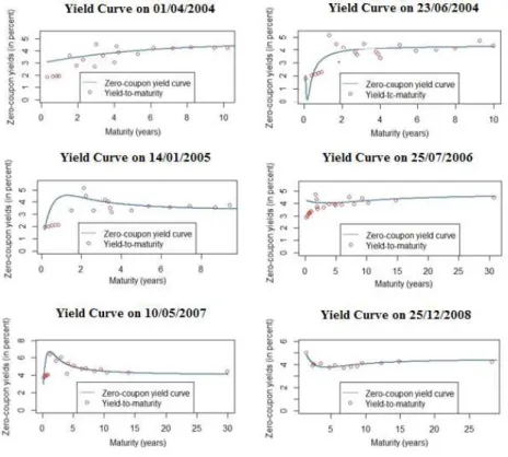
The Figure 1 and 2 depict several yield curve fitted by Nelson-Siegel model at

some specific dates throughout the period studied . As these yield curves show, the

Nelson-Siegel model is capable to capture different range of yield curve shapes: flat

or almost flat (e.g. yield curve on 01/04/2004 and 25/07/2006), upward sloping

(25)

Figure 1: Selected Fitted Yield Curve

yield curve on 23/06/2004, 14/01/2005 and 10/05/2007). In this case, the yield

curve depicts how the yield of the Portuguese Government Bond depends on its

maturity. Note that the slope of the yield curve depicts the gap between the short

and long term yields.

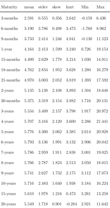
The Table A1 in the appendix, presents for varying maturities the descriptive

statistics of the estimated Portuguese Government Bonds yield curve that covers

the period from January 2004 through June 2014, such as mean yield, standard

deviation, kurtosis, skewness, minimum and maximum value achieved. Through the

analysis of these descriptive statistics, we can see that the yield curve on average

is upward sloping since the yields increase as the maturity increases, achieving its

(26)

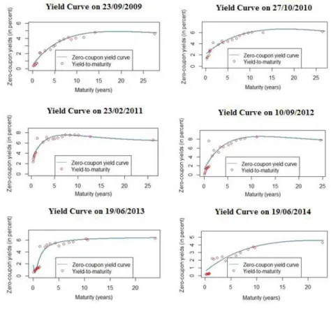
Figure 2: Selected Fitted Yield Curve (Continuation)

analysis, we conclude that on average the medium-term maturity is more volatile

than the short and long-term maturity, achieving its maximum at the maturity of

5 years; this means that, at some point, the volatility decreases as the maturity

increases.

The Table A2 in the appendix, details the basic descriptive statistics of the

parametersβ0, β1, β2, λt estimated by nonlinear least squares for each day t of the

period analyzed and in Figure 3 plots the evolution of each one of the parameters

estimated.

The β0, which can interpreted as long-term factor and defines the level of the

(27)

Figure 3: Evolution of Estimated Parameters over the period January 2004 through

June 2014.

maturity approaches to infinite. On average, β1 is negative, which means that

throughout the period from January 2004 to June 2014 the yield curve is on average

upward sloping. Theβ2, on average, is also positive and specified the position of the

curvature. The parameter more volatile is β2, which can explain that the curvature

of the yield curve is changing over time and in some cases the hump does not even

exist (e.g. yield curve on 19/06/2014, Figure 2). It is also important to stress the

ADF test done for each one of the parameters estimated. An Augmented version

of the Dickey-Fuller tests the existence of unit root for a univariate time series and

this result is particularly relevant for forecasting purpose. The more negative it is

the value of ADF, stronger is the rejection of the hypothesis that the univariate

time series has an unit root. Saying so, in this case the hypothesis of unit root is

rejected for all the parameters, which make the time series estimation appropriate

(28)

As the Figure 3 confirms, the curvature factor represented by β2 is the most

volatile parameter, especially in years 2009 to the end of 2013. Since the existence

of a ”hump” in the yield curve can be interpreted as a predictor of financial instability

and economic transition; the high volatility of parameter β2 may be explained by

the global financial crisis in July 2007 and by the impact of European Sovereign

debt crisis, consequently by the austerity measures applied in Portugal at 2011.

The primary objective of this study is to extract the term structure of yield

spread. Saying so, once the Portuguese yield curve is estimated, the yield spread

curve can be fitted using the disjoint method. In Figure 4 is depicted the yield

spread curve for varying maturities. Table A3 reports the descriptive statistics of

yield spread for varying maturities.

Figure 4: Portuguese Government Bonds Yield Spread over the period January 2004

through June 2014

In order to understand how the yield spread performs along the maturity

(29)

Table A3 in the appendix, we can see that, on average, the medium-term maturities

yield spread is higher than the shorter term maturities; however, at about 3-years

maturity the average yield spread tends to decrease as the maturity increases.

Re-garding the volatility of the mean yield spread, the medium-term maturities are

more volatile than the shorter and longer term maturity.

Figure 4 depicts the evolution of yield spread over the period January 1st _{2004 to}

June 30th_{2014 for the maturities of 3-months, 9-months, 1-year, 3-years, 5-years,}

10-years, 15-years and 20-years. Instead of depicts all the maturities analyzed in Table

A3, we chose references maturities in order to ease the graphical analysis. We can

see that until late of 2009, the yield spread has been following a stable pattern, with

some seasonal fluctuations. Afterwards, the yield spread rose steadily and peaked

in 2012. Taking into consideration the high level of yield spread experimented by

Portugal during this period, Portugal Government revealed a statement in January

15th _{2010 to reassure to investors that the government is committed to reduce the}

deficit. However, during the period from 2010 through 2012, the Portuguese

Gov-ernment Bonds credit spread of maturities of three and five years have still changed

significantly and reached a peak of about 20% in 2012. And during this period,

sev-eral credit agency lowered Portugal’s sovereign credit ranting by sevsev-eral notch. For

instance, in July 13th _{2010 Moody’s Investors Service lowered Portugal government}

bond rating from Aa2 to A1 and they pointed out the weak growth prospects faced

by Portugal; in March 29th _{2011 Standards & Poor’s downgrades the rating to}

BBB-from BBB; in April 1th _{2011 Fitch Ratings cutted the rating to BBB- from A-; in}

(30)

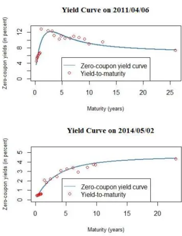
The yield curve estimated from observed prices and the yield spread are strictly

related. The Figure A1 in the appendix depicts the daily yield curve fit of year 2006,

as we can see in this figure the yield remains between 1% to 4% (with some peaks

reaching 5%); consequently, we can see in the Figure 4 that this period corresponds

to relatively low yield spread. Likewise, we can see in the Figure A2 and A3 (which

represent the daily yield curve fit of 2011 and 2012, respectively) that the yield is

increasing over time and reaching a peak of about 20% at the beginning of 2012

and the Figure 4 shows that the yield spread follows the same pattern. Once again,

through the analysis of the Figure A4 (daily fit of year 2014), we can see that the

yield and credit spread are positively correlated.

Not only Portugal, but other countries such as Ireland, Greece, Italy and Spain

have been affected by European Sovereign debt crisis, and consequently all of these

countries experimented significant changes in their yield spread, especially during

2012.

The Figure 5 shows the impact of the financial turmoil faced and the impact

of the austerity measures in Portugal. In April 6th _{2011 Portugal requested for a}

financial bailout from the European Union. As we can see in the first graph of the

Figure 5, the yields are already relatively high at the time of the request due to the

financial instability, Portugal’s government announcement about budget cuts and a

series of measures. In May 3rd _{2011 Portugal agreed with the European Union and}

the International Monetary Fund for ae_{72 billion financial bailout program. At the}

beginning of the program the yield spread increases significantly, especially yield

(31)

Figure 5: Impact of financial bailout on the yield curve

spread reached a peak about 20%). However, after several mission review during

the last three years, the yield spread has been following a decreasing pattern. The

second graph of the Figure 5 depicts the yield curve at the date of the final review

mission to Portugal and, as we can see, the yield reduced significantly and tends to

about 5% for long-term maturity Government bonds.

Moreover, it is also important to address the fitting errors. The price errors are

calculated as the difference between market bonds prices and its theoretical price

and the yield errors is computed as the difference between the bond yield and its

theoretical yield. Figure A5 and A6 in the appendix depict the price errors and

(32)

4.2 Out-of-sample Results 4 EMPIRICAL RESULTS

analysis of these two figures is noticed that the year that provided higher errors is

2012. These errors could be explained by different liquidity premium in the bond

market due to the conditions faced by Portugal described above.

4.2 Out-of-sample Results

As mentioned in the Section 3.2.2, the yield curve is forecasted by predicting the

estimated parameters of Nelson-Siegel model.

This research uses the Random Walk with drift as the benchmark forecast model

and as the competitor models the AR(1) and VAR(1). For each model, we use the

data from January 1st_{2004 to December 31}th_{2013 and the forecast begins at January}

1st _{2014 and go through June 30}th_{2014 for the forecast horizon of 1-month, 3-months}

and 6-months.

Regarding the benchmark Random Walk with drift, the regressions estimated is

presented in the Table 1 and the out-of-sample results can be found in Tables A4,

A5 and A6 for time horizon of 1, 3 and 6-month ahead, respectively.

By analyzing the regressions of the Random Walk with drift, the positive

non-zero constant term suggests that time series of β0,t and λ show an upward trend;

otherwise, the β1,t and β2,t suggest a downward trend. All the estimated drift

com-ponent is significant1_.

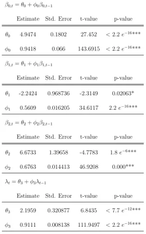
Relatively the AR(1), the regressions estimation are described in Table 2 and

the out-of-sample results are shown in Tables A7, A8 and A9 for forecast horizon of

1, 3 and 6-month ahead, respectively.

(33)

β0,t=α0+β0,t−1

Estimate Std. Error t-value p-value α0 0.000923 0.010713 0.086148 <2.2e−16***

β1,t=α1+β1,t−1

Estimate Std. Error t-value p-value α1 -0.000041 0.482021 -0.000085 0.000013***

β2,t=α2+β2,t−1

Estimate Std. Error t-value p-value α2 -0.00725 0.494452 -0.014657 <2.2e−16_***

λt=α3+λt−1

Estimate Std. Error t-value p-value α3 0.000069 0.029321 0.000047 <2.2e−16***

Table 1: Regressions estimated for Random Walk with Drift

The stationarity of the these time-series is proved by the value estimated forφi,

i=0,1,2,3, which is smaller than 1. Note that all the parameters estimated in AR(1)

are significant.

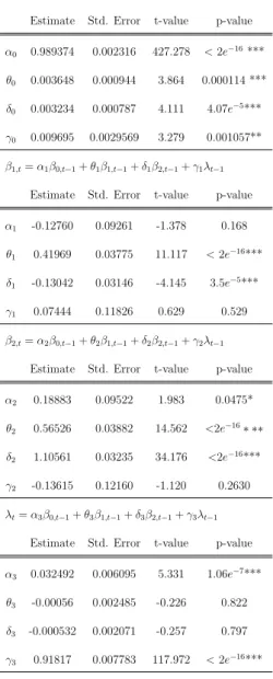
Lastly, the Table 3 details the matrix of regressions for the VAR(1) model and

the Tables A10 ,A11 and A12 display its out-of-sample results for the time horizon

of 1, 3 and 6-months ahead.

To assess the out-of-sample results, we use the yield fitted by Nelson-Siegel model

(1987) for the period of January 1st _{2004 through June 30}th _{2014. Using these yields}

we computed the RMSE for the maturities of 3-months, 1-year, 3-years, 5-years and

10-years. The RMSE is computed as:

RM SE =

v u u t 1 n n X t=1

(ˆyt−yt)2 (14)

which n stands for the number of observations, ˆyt stands for the forecasted yield

and yt stands for the yield extracted from the fitted yield curve.

(34)

β0,t=θ0+φ0β0,t−1

Estimate Std. Error t-value p-value

θ0 4.9474 0.1802 27.452 <2.2e−16***

φ0 0.9418 0.066 143.6915 <2.2e−16***

β1,t=θ1+φ1β1,t−1

θ1 -2.2424 0.968736 -2.3149 0.02063*

φ1 0.5609 0.016205 34.6117 2.2e−16***

β2,t=θ2+φ2β2,t−1

θ2 6.6733 1.39658 -4.7783 1.8e−6***

φ2 0.6763 0.014413 46.9208 0.000***

λt=θ3+φ3λt−1

θ3 2.1959 0.320877 6.8435 <7.7e−12***

φ3 0.9111 0.008138 111.9497 <2.2e−16***

Table 2: Regressions estimated for AR(1)

are quite similar. Both, depending the maturity and the forecast horizon, may

slightly outperform the results of the benchmark model. By comparing the RMSE

of AR(1) and VAR(1), we can observe that AR(1) seems to produce lower errors as

the maturity increases and this performance tends to improve as the forecasting time

horizon increases. This results agree with the Diebold and Li (2006) conclusions,

which argue that the forecasting models based on the Nelson-Siegel model perform

well and this performance improves as the forecasting time-horizon increases.

Regarding the forecasting model selection criteria, Table A13 shows the values

of log-likelihood, AIC and BIC (is a Schwarz criterion also known as Schwarz

(35)

β0,t=α0β0,t−1+θ0β1,t−1+δ0β2,t−1+γ0λt−1

α0 0.989374 0.002316 427.278 <2e−16***

θ0 0.003648 0.000944 3.864 0.000114 ***

δ0 0.003234 0.000787 4.111 4.07e−5_***

γ0 0.009695 0.0029569 3.279 0.001057**

β1,t=α1β0,t−1+θ1β1,t−1+δ1β2,t−1+γ1λt−1

α1 -0.12760 0.09261 -1.378 0.168

θ1 0.41969 0.03775 11.117 <2e−16_***

δ1 -0.13042 0.03146 -4.145 3.5e−5***

γ1 0.07444 0.11826 0.629 0.529

β2,t=α2β0,t−1+θ2β1,t−1+δ2β2,t−1+γ2λt−1

α2 0.18883 0.09522 1.983 0.0475*

θ2 0.56526 0.03882 14.562 <2e−16_{∗ ∗∗}

δ2 1.10561 0.03235 34.176 <2e−16_***

γ2 -0.13615 0.12160 -1.120 0.2630

λt=α3β0,t−1+θ3β1,t−1+δ3β2,t−1+γ3λt−1

α3 0.032492 0.006095 5.331 1.06e−7***

θ3 -0.00056 0.002485 -0.226 0.822

δ3 -0.000532 0.002071 -0.257 0.797

γ3 0.91817 0.007783 117.972 <2e−16_***

Table 3: Regressions estimated for VAR(1)

The model that exhibits a higher log-likelihood and that minimizes AIC and BIC

is considered the one which produces a better forecasts. Saying so, through the

analyses of values displayed in Table A13, one concludes that AR(1) is the model

that reveals a better forecast.

The underperformance of VAR(1) may be explained mainly by two reasons.

First, the regressions are estimated by OLS and when the parameters are

(36)

5 CONCLUSION

economic time series are highly correlated with its own past values and with the past

values of the other time series added in data set, a multicollinearity problem tends

to increase as more time series and lagged values are added in the model. Besides

that, the major drawback of VAR(1) is the fact that by increasing the number of

parameters to be estimated, higher will be the number of variables of the model.

5 Conclusion

The primary aim of this research is to fit the term structure of yield spread, focusing

on Portugal Government Bond over the period January 1st _{2004 through June 30}th

2014. To accomplish this objective, this study uses the disjoint method. Since

the latter method requires as an input a defaultable term structure and a

non-defaultable term structure, we estimated in daily basis the risky term-structure

based on Portuguese Government Bonds daily prices and using the Nelson-Siegel

model (1987). And we assumed as non-defaultable term structure the AAA-rated

curve of euro area government central banks, estimated by ECB using the Svensson

model (1994). Afterwards, the yield spread curve is obtained by the difference of

these two curves.

By analyzing the fitting results, we can see that some stylized facts of yield curves

are replicated in this research, such as: an upward sloping yield curve was the most

frequent shape estimated; the yield curves assumed several of shapes throughout

the time horizon (up sloping, humped and almost flat); some humped-shape curves

(37)

5 CONCLUSION

as the maturity increases.

Regarding the Portuguese Government Bonds Yield Spread, we conclude that

it followed a stable pattern, with some seasonal fluctuations, until the late of 2009.

Hereafter, the yield spread experimented a significant change, especially between the

end of 2009 to 2013. From the period 2009 to 2012, Portugal yield spread increased

sharply and spread of bonds with maturity of 3 and 5-years reached a peak of about

20% at the beginning of 2012. Afterwards, it started to decrease gradually until

2014, where the yield spread values are close to pre-crisis values. Note that the

period from 2009 to 2013 was precisely the years when Portugal faced a liquidity

and debt crisis. This weak debt and financial position leaded Portugal asks for ae₇₂

billion financial bailout from European Union and since then, Portugal was under

an Economic and Financial Adjustment Programme. After several mission review,

the final one was at May 2nd _{and since then, the yield spread seems to stabilize.}

Regarding the out-of-sample results, this research shows that the AR(1) and

VAR(1) slightly outperform the benchmark Random Walk with drift model. This

re-sult agrees with the conclusion of Diebold and Li (2006), which argued that forecasts

based on Nelson-Siegel model provides accurate results and this good performance

increases as the forecasting time-horizon increases.We also computed the forecasting

model selection criterions, which conclude that the AR(1) model provides a better

(38)

6 REFERENCES

6 References

Annaert, J., Ceuster, M. and Jonghr, F. (2000). Modelling European Credit Spreads.

Deloitte & Touche, Reaserch Report.

Berndt, A. (2003). Estimating the term structure of Credit Spreads Callable

Corporate Debt. Stanford University, Department of Statistics, Technical Report

2003-7.

Bjork, T. and B. Christensen (1999). Interest Rate Dynamics and COnsistent

Forward Rate Curves. Mathematical Finance, 323-348.

Bliss, R. R. (1997). Testing Term Structure Estimation Methods. Advances in

Futures and Options Researh (9), 197-231.

Bolder, D. and Str´eliski, D. (1999)Yield Curve Modeling at the Bank of Canada.

Bank of Canada, Technical Report 84.

Cochrane, J. H. and Piazzesi, M. (2002). Bond Risk Premia. Manuscript,

Uni-versity of Chicago and UCLA.

Diebold, F. X. and Li, C. (2006). Forecasting the Term Structure of Government

Bond Yields. Journal of Econometrics 130, 337-364.

Duffee, G. (1999). Estimating the Price of Default Risk. Review of Financial

Studies.

Duffee, G. (2002). Term Premia and Interest Rate Forecast in Affine Models.

The Journal of Finance 57(1).

Duffie, D. and Lando, D. (2001). Term Structures of Credit Spread with

(39)

6 REFERENCES

Duffie, D., Pedersen, L. H. and Singleton, K. J. (2003). Modeling Sovereign Yield

Spreads: A Case Study of Russian Debt. The Journal of Finance, 58(1), 119-159.

Duffie, D. and Singleton, K. J. (1999). Modeling Term Structure of Defaultable

Bonds. The Review of Financial Studies 12(4), 687-720.

D¨ullmann, k. and Windfuhr, M. (2000). Credit Spreads between German and

Italian sovereign bonds - do affine models work, Canadian Journal of Administrative

Sciences 17, 166-181.

Elton, E. J., Gruber, M. J., Agrawal, D. and Mann, C. (2001). Explaining the

Rate Spread on Corporate Bonds. Journal of Finance, 56, 247-77.

Fama, E. F. and Bliss, R. R. (1987). The Information in Long-Maturity Forward

Rates.The American Economic Review 77(4), 680-692.

Ferstl, R. and Hayden, J. (2010). Zero-Coupon Yield Curve Estimation with the

Package termstrc. Journal of Statistical Software 36(1).

Geyer, A. and Mader, R. (1999). Estimation of the Term Structure of Interest

Rates: a Parametric Approach. Austrian National Bank, Working Paper 37.

Geyer, A., Kossmeier, S. and Pichler, S. (2003). Measuring Systematic Risk in

EMU Government Yield Spreads. Review of Finance 8(2), 171-197.

Houweling, P., Hoek, J. and Kleibergen, F. (2001).The Joint Estimation of Term

Structures and Credit Spreads. Journal of Empirical Finance 8, 297 - 323.

Jeffrey, A., Linton, O. and Nguyen, T. (2006). Flexible Term Structure

Estima-tion: Which Method is Preferred? Metrika, 1-24.

Landschoot, A. V. (2004). Determinants of Euro Term Structure of Credit

(40)

6 REFERENCES

Linton, O., Mammen, E., Nielson, J. P. and Tanggaard, C. (2001) Yield Curve

Estimation by Kernel Smoothing Methods. Journal of Econometrics, Elsevier 105(1),

185-223.

McCulloch, J. H. (1975). The Tax-Adjusted Yield Curve. The Journal of Finance

30(3).

Molenaars, T. K., Reinerink, N. H. and Hemminga, M. A. (2013). Forecasting

the yield curve - Forecast performance of the dynamic Nelson-Siegel model from 197

to 2008. RiskCO BV, version 2.

Nelson, C. R. and Siegel, A. F. (1987). Parsimonious Modeling of Yield Curves.

The Journal of Business 60(4), 473-489.

Pooter, M. D. (2007). Modeling and Forecasting Stock Return Volatility and the

Term Structure of Interest Rates. Erasmus Universiteit Rotterdam.

Svensson, L. (1994). Estimating and Interpreting Forward Interest Rates:

Swe-den 1992-1994. National Bureau of Economic Research, Technical Reports 4871.

Vasicek, O. and Fong, H. G. (1982). Term Structure Modeling Using Exponential

(41)

Appendix

Descriptive Statistics of Portuguese Government Bonds Yield Curve

Maturity mean stdev skew kurt Min Max

3-months 2.591 0.555 0.356 2.642 -0.159 6.436

6-months 3.190 3.786 0.498 3.473 -1.768 8.962

9-months 3.733 2.414 1.246 4.841 -0.130 11.523

1-year 4.164 2.413 1.599 3.240 0.726 19.154

15-months 4.499 2.629 1.778 3.214 1.030 14.911

18-months 4.762 2.834 1.952 3.628 1.280 16.279

21-months 4.970 3.003 2.052 3.819 1.393 17.592

2-years 5.135 3.138 2.108 3.893 1.504 18.648

30-months 5.375 3.319 2.154 3.882 1.716 20.131

3-years 5.534 3.409 2.157 3.798 1.917 20.972

4-years 5.707 3.416 2.120 3.600 2.286 21.441

5-years 5.776 3.300 2.062 3.385 2.614 20.928

6-years 5.793 3.136 1.991 3.132 2.906 20.042

7-years 5.786 2.959 1.911 2.838 3.001 19.025

8-years 5.766 2.787 1.824 2.513 3.050 18.015

9-years 5.741 2.627 1.732 2.175 3.112 17.073

10-years 5.716 2.483 1.640 1.938 3.184 16.224

15-years 5.610 1.978 1.216 0.473 3.261 13.258

20-years 5.549 1.718 0.901 -0.284 2.921 11.642

Table A1: Descriptive Statistics of Portuguese Government Bonds Yield Curve.The

(42)

Descriptive Statistics of Estimated Parameters

Parameter mean stdev min max ρ1 ρ12 ρ30 ADF

β0,t 5.522 3.041 7.048e-09 21.529 0.963 0.714 0.486 -5.273

β1,t -3.790 3.557 -1.771e+01 28.013 0.986 0.559 0.248 -6.694

β2,t 5.216 14.702 -5.142e+01 62.634 0.973 0.674 0.194 -4.122

λ 2.842 3.937 6.134e-02 28.460 0.912 0.510 0.301 -6.2641

Table A2: Descriptive Statistics of Estimated Parameters, sample period: 2004:01

(43)

Descriptive Statistics of Portuguese Government Bonds Yield Spread

Maturity mean stdev min max Skew Kurt

3-months 0.759 1.231 -1.350 4.863 1.173 1.028

6-months 1.493 1.726 -1.840 8.415 1.922 3.162

9-months 2.076 2.226 -0.207 11.123 2.040 3.532

1-year 2.506 2.654 -0.013 13.055 2.039 3.455

15-months 2.823 3.008 0.006 14.391 2.007 3.261

18-months 3.056 3.295 0.033 15.944 1.966 3.047

21-months 3.228 3.524 0.065 17.194 1.924 2.845

2-years 3.353 3.704 0.095 18.182 1.884 2.665

30-months 3.504 3.944 0.159 19.519 1.812 2.373

3-years 3.566 4.066 0.217 20.204 1.751 2.153

4-years 3.535 4.093 0.305 20.318 1.653 1.833

5-years 3.400 3.970 0.285 19.510 1.569 1.574

6-years 3.224 3.786 0.202 18.319 1.491 1.327

7-years 3.038 3.586 0.108 17.025 1.416 1.079

8-years 2.858 3.391 -0.048 15.770 1.342 0.835

9-years 2.693 3.209 -0.189 14.617 1.271 0.598

10-years 2.544 3.046 -0.312 13.589 1.204 0.378

15-years 2.047 2.483 -0.724 10.135 0.932 -0.432

20-years 1.829 2.215 -0.949 8.451 0.749 -0.834

Table A3: Descriptive Statistics Portuguese Government Bonds of Yield Spread.

(44)

Out-of-sample Results: Random Walk with Drift

Maturity mean stdev RMSE ρ1 ρ12

3-months 2.273 0.003 0.697 0.864 -0.251

1-year 0.911 0.004 1.927 0.728 -0.313

3-years 0.624 0.009 2.282 0.595 -0.395

5-years 1.687 0.007 2.070 0.466 -0.414

10-years 3.814 0.002 1.405 0.438 -0.360

Table A4: Out-of-sample Forecasting Results, RW with drift: 1-month ahead

3-months 2.282 0.008 0.677 0.886 0.2611

1-year 0.899 0.011 1.930 0.863 0.222

3-years 0.595 0.025 2.289 0.729 0.146

5-years 1.662 0.022 2.076 0.641 0.184

10-years 3.805 0.007 1.400 0.596 0.146

Table A5: Out-of-sample Forecasting Results, RW with drift: 3-month ahead

3-months 2.296 0.016 0.667 0.841 0.488

1-year 0.881 0.021 1.935 0.864 0.467

3-years 0.552 0.050 2.298 0.886 0.445

5-years 1.624 0.043 2.085 0.751 0.424

10-years 3.793 0.0145 1.412 0.774 0.403

(45)

Out-of-sample Results: AR(1)

3-months 1.448 0.098 1.043 0.121 -0.151

1-year 3.721 0.124 1.630 0.720 -0.163

3-years 6.097 0.197 1.676 0.846 -0.248

5-years 6.715 0.209 1.601 0.324 -0.162

10-years 7.137 0.283 1.499 0.367 -0.171

Table A7: Out-of-sample Forecasting Results, AR(1): 1-month ahead

Maturity mean stdev RMSE ρ3 ρ18 3-months 1.547 0.087 1.089 0.851 0.176

1-year 3.547 0.151 1.576 0.811 0.154

3-years 5.743 0.303 1.567 0.831 0.172

5-years 6.350 0.347 1.482 0.838 0.181

10-years 6.6719 0.435 1.335 0.846 0.193

Table A8: Out-of-sample Forecasting Results, AR(1): 3-month ahead

3-months 1.590 0.074 1.073 0.747 0.186

1-year 3.469 0.133 1.075 0.725 0.249

3-years 5.580 0.270 0.503 0.739 0.243

5-years 6.141 0.324 0.410 0.771 0.288

10-years 6.345 0.452 0.748 0.801 0.345

(46)

Out-of-sample Results: VAR(1)

3-months 1.243 0.026 0.940 0.709 -0.291

1-year 3.456 0.194 1.546 0.827 -0.264

3-years 6.051 0.193 1.662 0.835 -0.269

5-years 6.853 0.148 1.643 0.834 -0.268

10-years 7.321 0.168 1.559 0.851 -0.287

Table A10: Out-of-sample Forecasting Results, VAR(1): 1-month ahead

1-year 3.368 0.132 1.518 0.636 -0.141

3-years 5.943 0.139 1.630 0.672 -0.125

5-years 6.761 0.107 1.615 0.669 -0.097

10-years 7.077 0.206 1.478 0.669 -0.097

Table A11: Out-of-sample Forecasting Results, VAR(1): 3-month ahead

1-year 3.563 0.268 1.061 0.309 -0.039

3-years 5.968 0.457 0.135 0.086 0.002

5-years 6.622 0.514 0.649 -0.007 0.026

10-years 6.789 0.316 1.003 0.370 0.229

(47)

Forecasting Model Selection Criteria

Random Walk with drift

Selection Criteria β1,t β2,t β3,t λ

log-likelihood -2152.85 -12034.08 -12100.38 -4595.53

AIC 4307.69 24070.15 24202.76 9193.06

BIC 4313.89 24076.02 24208.63 9198.9

AR(1)

log-likelihood -2086.48 -11715.62 -11875.13 -4540.19

AIC 4178.96 23437.24 23756.26 9086.38

BIC 4196.55 23454.84 23773.86 9103.9

VAR(1)

log-likelihood -24151.55

AIC 48367.11

BIC 48554.78

Table A13: Forecasting Model Selection Criteria computed for the RW with drift,

(48)

Portuguese Government Bonds Daily Yield Curve Estimation

Figure A1: Portuguese Treasury Bonds Yield Curve daily fit of year 2006.

(49)

Figure A3: Portuguese Government Bonds Yield Curve daily fit of year 2012.

(50)

Price Errors of the Yield Curve Estimation

Figure A5: Pricing errors generated by estimating the yield curve over the period

January 1st _{2004 through June 30}th _2014.

Yield Errors of the Yield Curve Estimation

Figure A6: Yield errors generated by estimating the yield curve over the period