Spatial distribution of local economic performance: empirical analysis of employment, income and poverty in Brazilian municipalities

Empirical Analysis of Employment, Income and Poverty in

Brazilian Municipalities

Ciro Biderman

and Danilo Igliori

α

_{Getúlio Vargas Foundation, Lincoln Institute of Land Policy and MIT}

_{University of Sao Paulo and University of Cambridge (corresponding}

author: [email protected])

Abstract

Local economies within a country differ substantially in their economic performance and such differences might persist over long periods of time. Increasing concern with regional disparities and poverty levels have prompted a growing interest in understanding factors giving some places better conditions for enhancing performance and overcoming development challenges. In particular, researchers and policy makers have been trying to investigate the potential roles of public policy at local level. Here, the key question relates to the capability of local governments in significantly impacting their realities despite their historic, economic, social and geographical constraints. The central aim of this paper is to empirically investigate the factors influencing local development across Brazilian municipalities, emphasizing the role of local public policy. To do that we adopt spatial econometric models inspired by growth theory and by some recent development of spatial economics. Our results contribute to the identification of determinants of local economic development measured by three variables, namely employment change, income per capita change and the change in the population below the poverty line. From the empirical estimates evidence is provided regarding the factors suggested by the recent literature on growth, development and spatial economics.

This is a draft of a work in progress. Please do not quote

or circulate.

Spatial Distribution of Local Economic Performance: An

Empirical Analysis of Employment, Income and Poverty in

Brazilian Municipalities

Ciro Biderman

and Danilo Igliori

1. Introduction

Local economies within a country differ substantially in their economic performance and such differences might persist over long periods of time. Although differences in local development performance have always been a familiar feature of the economic landscape, increasing concern with regional disparities and poverty levels have prompted a growing interest in the factors giving some places better conditions for enhancing performance and overcoming development challenges. Moreover, researchers and policy makers have been trying to further understand the related role of public policy at local level. Here, the key question relates to the capability of local governments in significantly impacting their realities despite their historic, economic, social and geographical constraints. The central aim of this paper is to empirically investigate the factors influencing local development across Brazilian municipalities, emphasizing the role of local public policy. To do that we adopt spatial econometric models inspired by the neoclassical growth theory and by some recent development of spatial economics.

Empirical evidence suggests correlations between the proportion of expenditure in education, health or infrastructure expenditures and municipal performance cannot be presumed to be correlated with other initial characteristics. There is enough variance in the sample that gives us a good opportunity to estimate the trade-offs between two classes of expenditures at the local level—education and health spending and infrastructure (energy, transportation, housing, and regional development) spending. However, to measure the implicit trade-offs, we need a measure of the goal of these programs. We believe that a program of LED should have as a basic purpose the improvement of well-being of its residents. While the fundamental concern is with equity and development, the empirical investigation utilizes the population below the poverty line as a proxy for inequality and per capita income as a measure of growth. Program goals often appear among the objectives that should be means and not final objectives. In particular, it is common to find employment, income generation, firm recruitment or the support for local companies among program objectives. This would be a justifiable objective if there were some production scale gains. Thus, the increase of the scale of the municipality would generate productivity gains and consequently increase the well-being of its residents. For that reason, to measure the performance of a local public policy we will look at employment variation as well.

The way we are analyzing public policy at the local level parallels empirical analysis on convergence across municipalities. We want to know which combination of policies leads a municipality converge towards the average level of income, poverty or employment generation at the fastest rate. The empirical analysis of income convergence departs from the classical theory of economic growth. The main idea is that in regions with a smaller stock of capital this factor should be more productive than in regions with a larger stock of capital. So, the argument goes, capital would flow from over-capitalized regions to under-capitalized ones and income would converge within regions. This hypothesis is called “absolute convergence”. One variation of the hypothesis, known as “conditional convergence” states that given differences in preferences or initial conditions, regions may converge to a different level of income. The main findings in Brazil and in many other places is that while conditional convergence is very close, absolute convergence will take a very long time to happen.

In this report we are not worried about whether absolute or conditional convergence occurs, but rather, whether local policies affect the rate of growth. However, given the high pace of conditional convergence, if we did not control for initial conditions we may be neglecting a highly significant variable. Actually, the convergence component is one of the highest determinants for any goal (growth, poverty reduction or employment generation). For income per capita, we confirm the conventional wisdom that we are very close to convergence (less than 2 years) and we find some indirect evidence of convergence clubs, i.e., some municipalities are converging to a lower level and others converging to a (relatively) higher level. Convergence in employment captures the congestion costs (firms leaving very concentrated regions). Convergence in population below the poverty line means that poor migrants are leaving the municipalities with a (relative) high proportion of poor to regions with a lower proportion. We test our results using different statistical methodologies and the results are very robust to any methodology adopted.

Our results contribute to the identification of the determinants of local economic development measured by three variables, namely employment change, income per capita change and the change in the population below the poverty line. From the empirical estimates evidence is provided regarding the factors suggested by the recent literature on growth, development and spatial economics. The remaining of this paper is structured as follows. The next section provides the analytical framework guiding our empirical analysis. Section 3 describes the data and variables used in the estimations. We then present the results and conclude contrasting our findings with potential policy implications. Then we specify the model that we will be running and explain the methodological aspects connected to the use of spatial interactions. Another appendix presents detailed regression results. We include these sections in the appendices for the more technical reader who is interested in following the formal arguments and checking the main technical hypothesis underlying the reported simulations. In the technical appendix we formally derive the convergence model.

2.

Analytical Framework

Our concern with public policy at local level relates to the so-called ‘convergence theory’ put forward by the early neoclassical growth models. In other words we aim to understand what are the factors contributing to the movement of a particular locality towards the national average. The per capita income convergence hypothesis can be summarized as the tendency of a continuous reduction in the differences between more or less advanced economies. The presence of convergence is perhaps the main result coming from the models developed by Solow (1956) and Swan (1956). This is due to the existence of decreasing returns to scale of production inputs. Recent studies however point out that different regions might converge to equally different steady-state income levels and alert for the importance of studying the determinants of steady-state growth rates across different economic realities. Subsequent studies have pointed out that regions will not necessarily converge towards the same steady-state income level. In other words, smaller regions with initial per capita income may grow at higher rates, which do not imply that the equilibrium growth rate (steady-state rate) will be equal to that of regions with greater initial levels of per capita income. Some authors state that the Solow model implies identical growth rates for all regions. However, there is a consensus today that this result is fully compatible with the resulting hypothesis of the Solow model as this model was not developed to examine growth rates between regions, but rather within a single region.

This controversy led to the need to examine the conditional determinants of the steady

state growth rates of each region and how such factors affected this growth. These

studies remained known as conditional convergence studies (Barro and Sala-i-Martin 1995), while previous studies are often characterized as absolute convergence studies. It should be noted that these studies help explain the non-occurrence of absolute convergence between regions. This is because regions differ in their conditioning growth factors and, thus, factors that can be crucial for economic growth may be much more present in developed regions with higher initial levels of per capita income than in regions that, in the initial period, had lower per capita income levels. However, it should be emphasized that the dimension of high per capita income or low per capita income is defined according to the regions that comprise the selected sample.

Also it should be emphasized that empirical studies have examined how institutional factors have conditioned per capita income growth (or of the convergence/divergence of income). Gallup, et. al. (1999) try to relate political and geographical factors to economic performance in developing countries. In general, regions localized close to the coast or close to major navigable rivers presented higher growth rates than others over time. In addition, countries with greater political instability (greater rates of inflation, smaller participation of the population in the decision-making processes, etc.) also presented lower growth rates. For Brazil, in general, the factors that are most frequently cited in the literature pertain to human capital, local infrastructure, the degree of specialization of economic activity (Azzoni, 1998; Azzoni, et. al. (2000); Andrade and Sierra 1998; Chagas and Toneto Jr., 2002).

There are several studies that address convergence patterns in Brazil. The majority of these studies aim to test the existence of convergence rates among Brazilian states, mainly with respect to per capita income, but do not achieve a consensus with to the speed of convergence. Ferreira and Diniz (1995), Schwartsman (1996) and Zini Jr. do not reject the hypothesis of absolute convergence in per capita income for Brazilian states for the period between 1970 and 1985. Azzoni (1997)(2001), using a longer series (1939-1996), also finds indications of absolute convergence of income, but at a much smaller rate.1 In response to Azzoni (1997), Ferreira (1998) estimates Markov transition matrices for state GDP data between 1970 and 1995 and finds convergence evidence. Porto Jr. and Ribeiro (2000) find convergence evidence across states in the period between 1985 and 1998 and in municipal growth in the South between 1970 and 1991.

All of the studies cited in the previous paragraph utilize states as the unit of analysis. Other studies have tried to find convergence evidence at a smaller scale. Azzoni et. al. (2000) find conditional convergence in income between metropolitan regions in Brazil, while Andrade and Sierra (1998) suggest the existence of convergence among average municipalities in Brazil between 1970 and 1991. Chagas and Toneto Jr. (2002) report the existence of conditional convergence for Brazilian municipalities between 1980 and 1991. Andrade, Laurini and Pereira (2005) analyzing the evolution of the relative distribution of per capita income for Brazilian municipalities in the period from 1970 to 1996, utilizing a Markov transition matrix, detect the formation of two convergence clubs, a low-income group formed by municipalities in the Northern and Northeastern regions, and another high-income group formed by municipalities in the Midwest, Southeast, and South regions.

In contrast to Neo-Classical growth models of the Solow variety, which emphasized capital investment and exogenous technological change to explain differences in growth across nations, regions and cities, the more recent research on growth focuses on externalities as the ‘engine of growth’ and in particular on the role of local knowledge externalities as sources of increasing returns. This approach has its origins in the work by Romer (1986), and his revival of the early work by Arrow (1962) on learning by doing, extending the latter to include investment in knowledge. Lucas (1988), adopting a somewhat different approach reaches a similar conclusion. For instance, the so-called Marshall-Arrow Romer (MAR) externalities relate to knowledge spillovers between firms in an industry and this view applied to cities implies that urban concentrations of firms facilitates such spillovers (Glaeser, Kallal, Scheinkman, and Shleifer 1992). Porter (1990) likewise emphasizes the importance of intra-industry knowledge spillovers. On this view, industry specialization favors city growth. By contrast, for Jacobs (1969) it is inter-industry knowledge spillovers that matter most and it is urban industrial diversity that is important for growth. NEG Models provide further insights into the dynamics of urban growth. Krugman (1991) for example, working within the framework of the NEG has emphasized the importance of dynamic externalities for our understanding of spatial patterns of growth but has downplayed their importance except in the case of localities

1 _{Some of these works (Azzoni 2001; Schwartsman, 1996; Zini Jr., 1998) utilize the same methodology}

of Mankiw, Gregory. 1982.estimating a series of regressions in order to identify the determinants of growth differentials among countries.

dominated by high-technology industries. Krugman’s (1991) Core-Periphery (CP) model focuses therefore on increasing returns, pecuniary externalities and transport costs. The mechanics of the model are driven by three effects: market access, cost of living, and market crowding. As summarized by Baldwin et al (2003), the ‘market access effect’ describes the tendency of monopolistic firms to locate their production in the big market and export to small markets; the ‘cost of living effect’ concerns the impact of firms’ location on the local cost of living (goods tend to be cheaper in regions or cities with more industrial firms since consumers will import a narrower range of products and thus avoid more of the trade costs); the ‘market crowding effect’ reflects the fact that imperfectly competitive firms have a tendency to locate where there are relatively few competitors.

The first two effects encourage spatial concentration while the third discourages it. Combining the market-access effect and the cost-of-living effect with interregional migration creates the potential for ‘circular causality’ – also known as ‘cumulative causation’. The natural question is therefore what determines the relative strength of these forces. Trade costs play the key role in balancing centripetal and centrifugal forces. As trade costs decline both dispersion and agglomeration forces diminish. Competition from firms outside the locality becomes approximately as important as competition from locally based firms and there will be very little spatial difference in prices between the two areas.

Building on the NEG approach, Baldwin et al (2003) propose an endogenous growth model, in which long run accumulation of knowledge capital is supported by learning effects from an innovation sector that has a public good component. In the local spillovers version it is assumed that knowledge spillovers dissipate with distance. These models of growth and agglomeration provide analytical underpinning for empirical models using a variety of spatial econometric methods (Abreu, Groot, and Florax 2004; Fingleton 2003).

The recent literature on spatial economics has emphasized the role of agglomeration and clustering of economic activities as fundamental causes of an enhanced level of local economic performance, creating externalities that cause firms to grow faster and larger than they otherwise would do. One important consideration in spatial economics is that the positive externalities generated by agglomerations could be offset to some degree by negative externalities due to congestion effects. Congestion is most likely in the densest agglomerations, so that it is an interesting empirical question to examine whether the balance of positive and negative externalities swings in favor of congestion effects at the higher levels of agglomeration. A second fundamental idea lies on the relevance of transport costs for generating unequal patterns of distribution of economic activity. Here, proximity to markets for both inputs and outputs are central to explain growth and development of cities.

Although our approach is clearly related to the literature outlined above we have objectives that go beyond issues related to convergence or GDP growth. Firstly we are not interested in finding whether there is absolute or conditional convergence between the municipalities. Our primary question looks at the influence of local policy in economic development. In addition we aim to examine the dynamics of other variables regarding local welfare such as poverty levels and employment. The great difficulty is in expanding this approach to the study of objectives other than growth

rates, such as poverty reduction. The objectives of local policy do not merely seek to increase productivity, income, or employment. Some local policies are concerned with poverty reduction. In this study it is assumed that the results are simply a measure of convergence and accept that we can also use the same measure to study the impact of policy on poverty reduction. The coefficient of the lagged dependent variable indicates whether convergence is occurring. The coefficient of public policies indicates if these variables are increasing or decreasing the rate of convergence. These are the equations we seek to test.

Nevertheless, there are two means by which a municipality can increase income and employment or reduce poverty. It can implement policies that increase its productivity or policies that “steal” firms or “expel” its poor households to other municipalities. In other words, the interaction between neighbors is fundamental for the characterization of development policies at the local level. In order to incorporate neighborhood effects we expand the empirical models along the lines suggested by spatial econometrics.

3. Data and Variables

The first difficulty in the construction of the database is to define the unit of analysis. For our ends, we would ideally want to work at the scale of the municipality, the only effectively “local” scale. However, between 1991 and 2000 the number of municipalities in Brazil increased from 4,491 to 5,507. In order to obtain a consistent panel of districts for this period, we utilize the IPEA definition of “Minimum Comparable Areas” (AMC) as our unit of analysis. Given the increase of 1,106 municipalities in the period, IPEA’s effort is remarkable since it succeeded in creating 4,267 comparable areas between in both periods. This is the most detailed scale that is possible for Brazil in the 1990s decade. Actually as can be observed in Table 1, 85% of AMCs only had one municipality while 10% had 2 municipalities. In other words, the quantity of AMC with 3 or more municipalities is very low.

Table 1. Number of Municipalities in each AMC

Number of Municipalities Percentage 1 84,71% 2 10,27% 3 2,30% 4 1,24% 5 0,56% More than 5 0,91% Source: IPEA

This type of analysis by AMC, to our knowledge, has not been carried out in any other study. Some studies have worked on the municipal scale as Laurini, Andrade, and Pereira (2003). The authors, however, did not utilize AMC and, therefore, simply eliminated the municipalities that altered their composition during the period.2 As we

2 _{It is not clear if the authors controlled for changes in municipalities that maintained the name but lost}

are controlling for spatial correlation, the elimination of municipalities would substantially alter the analysis. Lall and Shalizi (2003) also work with municipalities, but remain restricted the municipalities of the Northeast.3 Thus, we believe that this is one of the new developments of this study and, therefore, one of the contributions for the literature.

For our survey objective, working at the municipal scale is fundamental. In addition, research limited to one given region can also distort the results. This is because the interaction among municipalities, say, of the Northeast, is not necessarily restricted to the region. It is clear that it could be said that upon limiting our analysis to Brazil we lose, for example, the interaction with municipalities in Argentina. Nevertheless, there are much greater barriers in international than in national relations. Moreover, there are reasons to believe that given Brazil’s low share of international trade in general and in particular with Latin American countries (except for Argentina), the size of these distortions is relatively small in comparison to those that would result from isolating a given region.

The data for this analysis is from a number of sources. Firm and employment data were obtained from the the Relação Anual de Informações Sociais (RAIS), compulsory information collected annually by the Ministry of Labor and Employment (MTE) at the firm level. Have access to micro-data from the RAIS, i.e. the information at the company level thanks to an agreement with the department of statistics of the MTE. It was possible to calculate, for example, the number of firms created and closed during the period. Data at the municipal scale or, when available at the AMC level, were obtained from UNDP/IPEA, IBGE and IPEA (for public finance accounts data was obtained from the Secretaria do Tesouro Nacional – STN). When the data were only available at the municipal scale, they were re-aggregated by AMC guaranteeing comparison across time.

Three different dependent variables were tested to explain the change in local development between 1991 and 2000 measured as the difference in the log value of the selected variable in the final year, 2000, subtracted from its log value initial year, 1991. We choose growth rates rather than levels to avoid spurious correlations. The three dependent variables are growth in per capita income, growth in the total number of workers employed in the formal market labor force, the percentage of households earning income less than R$ 75.50 per capita. Each of these dependent variables was selected to capture an important component of local economic development guided by the literature review conducted for this study.

Depending on which of the three dependent variables was selected for the specification, we include the lagged log value of the dependent variable in 1991 as an independent variable. For example, if the growth in formal employment between 2000 and 1991 is the dependent variable, we utilize the log of employment in 1991 (EMPREGO_91). We include the lagged dependent variable to control for convergence between districts. In particular, we seek to control for whether the correlation between initial employment levels and employment growth (convergence) occurs or whether agglomeration forces may cause advanced cities to grow at faster rates.

3 _{Also in this case it is not very clear as the authors struggled with the new municipalities created in the}

It is important to emphasize that the selection of employment data for Brazil included in our specification captures formal labor market participation. In our view, this measure is more adequate than a measure that also includes informal employment. As the primary goal of employment generation is the inclusion of workers in the formal economy, we believe this measure is more adequate. One problem with using formal employment data based on RAIS is that this variable is based on the location of employment and not the worker’s AMC of residence. In agglomerations, such as São Paulo, we suspect that there are considerable differences between the location of firms and worker’s residencies, a feature that may be particularly important to capture in our model. In future iterations, we hope to further test these specifications with data that examine whether there are considerable differences when alternative data sources that permit to control for employment levels based on worker’s residence are available.

In order to control for similarities between AMC districts, we include variables to capture the initial conditions in each district. We have selected a set of control variables that could have direct or indirect impact on municipal development. In selecting the control variables, we seek to control for both initial socio-economic and geographic conditions in Brazilian localities. Individual significance, global likelihood, and correlation between the explanatory variables of several alternative combinations oriented the variable selection for the final model.

The first set of variables control for socio-economic conditions. The vector of initial conditions,Χ , includes the log of the population in 1991 (linear and squared) to control for district population size (POP_91). To control for the level of human capital, we include the log of the mean educational level of adults 25 years or older in the regressions (ANOS_ESTUDO_91). To control for the level of social inclusion, we include a measure of the percentage of households earnings incomes less than R$ 75.50 per capita (POBREZA_91) as calculated by UNDP. In relative terms, R$ 75.50 was equivalent to earning half the level of a minimum wage salary in August 2000. As we suspect that spatially specific characteristics such as access to markets, we include a second set of variables seeks to capture geographic conditions. We include the log area of the AMC to control for district size (AREA_91). In addition, a dummy variable to capture costal district status (COSTEIRA) and measures of the distances to São Paulo (DIST_SP_100) and the state capital (DIST_CAP_100) were included to capture transport costs and market access. Dummies for each of Brazil’s 25 states were included in the specifications with São Paulo dropped from the sample.

Since the primary objective of the study is to examine the impact of local economic development initiatives, we test to see the association between Brazilian municipal government expenditures in human and physical capital have an impact on levels of regional development after controlling for initial and geographic conditions. All data on municipal expenditures are for 1994. We did not use data for earlier years due to problems in the data collection in earlier years, which lead us to believe that the data are less reliable. As measures of local government policies that emphasize human capital investments, we include both the share of expenditures on health (P_SAUDE) and education (P_EDUC) as a percentage of total spending. To measure the share of investments in physical capital as a share of total spending, we combine four types of infrastructure: energy, transportation, housing and regional development (P_INFRA).

As state transfers compromise a significant share of spending for some municipalities, we also include a measure to examine whether there are differences in AMC growth performance in those districts that depend primarily on state transfers (P_TRANSF). We believe that this is an important measure to capture and explore as most state transfers are pre-targeted to specific expenditure categories and therefore give local governments less discretion in spending.

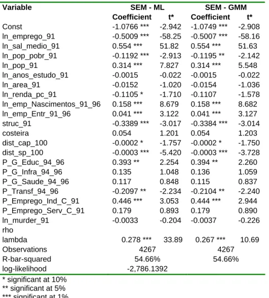
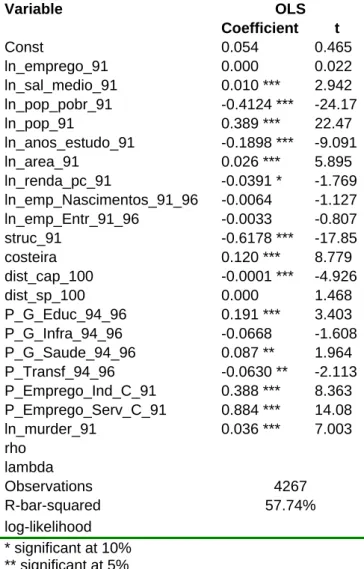
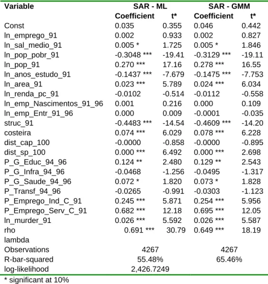
4. Results

We have estimated spatial models aiming to provide evidence of the determinants of change in development performance (employment, income and poverty) for Brazilian municipalities between 1991 and 2000 with emphasis on the role of local public policy. The estimated coefficients in the seven models (ordinary least squares and six spatial models as discussed in the appendix) for each of our dependent variables are robust as they are generally similar in value and significance. The spatial lags for the dependent variable and the error term are highly significant in all specifications, indicating that controlling for spatial autocorrelation is important in this empirical methodology. Given the similarities across the estimated models and provided that both of the spatial coefficients (for the error term and for the spatial lag) are simultaneously significant, we would base the following discussion on the results for the general spatial model (SAC). The tables in appendix 3.D present the estimates for all the models.

As discussed above, our specifications correspond to a test for convergence across AMCs. Maps 3.1 to 3.3 present the spatial distribution of the 3 dependent variables together with the scatter diagrams between the variation of employment, income per

capita and population below the poverty line between 1991 and 2000 and their

respective levels in 1991.

During the 1990s aggregate income per capita in Brazil was growing slowly, repeating the bad performance of the 1980s. In this context, a modest growth may be considerable in relative terms. However, the average growth of Brazilian municipalities was reasonable, around 3.8% per year. This apparent contradiction is due to the fact that the most populated municipalities have grown slower than the less populated ones.

Map 3.1 shows that there were actually signs of absolute convergence for some groups (or clubs). The Map split the municipalities in four groups: Municipalities that had above average income per capita on 1991 and that grown at a faster than average pace between 1991 and 2000 (HH); Municipalities that had bellow average income per capita on 1991 and had grown at a faster than average pace between 1991 and 2000 (LH); Municipalities that had above average income per capita on 1991 and had grown at a slower than average pace between 1991 and 2000 (HL); and Municipalities that had bellow average income per capita on 1991 and had grown at a slower than average pace between 1991 and 2000 (LL).

Map 3.1: Income per capita Variation in Brazilian Municipalities (1991-2000)

Source: Elaborated by Cepesp using data from Ibge and Ipea.

The geographical distribution of income per capita variation with groups defined as above provides a clear picture of absolute convergence. The LH group represents the group catching up and the HL group represents the rich municipalities adjusting for fast growth in the past and a (relative) over stock of capital. The HH and LL group are diverging but the two groups are rather different. We might expect some municipalities on the HH group since we have economies to scale and a fast growing region might continue to grow for some decades. The LL group might be in what we call a “poverty trap”. That is, the LH and HL groups are the convergent municipalities and the HH and LL are the divergent ones.

The good news is that the LH group is the largest. There were more municipalities catching up during the 1990s in Brazil than anything else. Unfortunately the smallest group is the HH. Actually, the difference between the number of municipalities in the HH group and the LL group is much higher than the difference between the LH and the HL group. These counts are showing that part of the convergence observed in Brazil during the 1990s is due to the modest performance of some relatively rich municipalities. In particular, most of the municipalities in the State of São Paulo were in the HL group.

On the other hand, most of the municipalities in the LH group were in the northeast. However, we cannot be so optimistic about this result. First, most of the municipalities with income per capita bellow the average were in the northeast on 1991. Second, most of the municipalities in the LL group were also in the northeast. For instance, almost all municipalities in Alagoas and Sergipe and a considerable share of municipalities in Pernambuco and Maranhão were in the “poverty trap” group. Third, we can see that the municipalities on the LH group in the northeast are normally in the countryside rather than close to the coast. Since income in the

countryside of northeast is lower than in the coast, those are good news, however, combined with the high incidence of municipalities in the LL group in the northeastern coast, the municipalities in the northeast may be converging to a low income level. As a matter of fact, Andrade et al. (2004) found evidence of “club convergence” in Brazil during the 1990s.

A similar picture is depicted with respect to employment, as there is strong evidence of absolute convergence. The municipalities are actually concentrated in the northwestern and southeastern quadrants indicating that the majority of municipalities above the mean reduced employment while the municipalities below the mean created jobs. It is interesting to observe again that municipalities along the coast are reducing employment while those municipalities in the interior are increasing. The question of how much of this non-conditional convergence is desirable is a complicated issue since losses may be wasting agglomeration gains. On the other hand, some congestion costs may be being avoided.

Map 3.2: Employment Variation and Initial Employment

The degree of poverty of municipalities measured by the population below the poverty line does not show signs of absolute convergence. In fact, we have evidence to the contrary. A greater number of municipalities that were above the mean of population below the poverty line experienced an increase in their share of this population than municipalities who reduced this index. The number of municipalities that increased the degree of poverty is similar to those who reduced among the municipalities who were below the mean of population below the poverty line.

The conditional convergence hypothesis is also evidenced by the econometric estimations since the coefficient of the lagged variable is always negative and significant at 1% of statistical significance. Moreover, the estimated convergence term have one the highest magnitude among the control variables for the 3 dependent

variables. It is interesting to note that, controlling for a number of socio-economic and geographical characteristics, positive (employment and income) but also negative (poverty) changes are suggesting the existence of a less concentrated process in terms of local development. The case of poverty is particularly interesting as convergence is evidenced when controls are introduced.

As suggested by the literature on spatial economics the estimates for population, controlled for area size, are significant. These results provide evidence that on one hand agglomeration intensity is relevant for local economic development and, on the other, that congestion costs played a significant role during the 1990s. Our specifications do not allow us to identify what kinds of agglomerations effects are working in the case of Brazilian municipalities and distinguish potential impacts of microeconomic characteristics such as market size, public facilities sharing, better matching between firms and workers or knowledge spillovers (see Duranton and Puga [2004] for a discussion about micro foundations of agglomeration economies). Possibly we would find most of these factors in a greater or lesser extent depending on the local conditions.

Map 3.3: Variation in the Population below the Poverty Line and Initial Population

Spatial economics suggest that the relationship between initial population densities and subsequent development is non-linear. We should expect significance for both the linear and quadratic terms, with positive coefficient for the linear variable and negative for the quadratic one. For low levels of agglomeration larger population contributes to economic performance but perhaps would also enhance the attractiveness for poor people. However, at higher levels of agglomeration congestion effects start to ‘quick in’ producing negative externalities, reducing growth and development. Curiously we found evidence of this pattern only in the poverty

regression. In the employment and income per capita regressions only the quadratic term is significant and positive.

These results reveal that for most of the municipalities congestion is not a problem if we control for all other variables. On the contrary municipalities with same initial characteristics are still benefiting considerably from agglomeration economies. Given the number of variables included in the analysis we cannot say anything about the constant term. In any case, the fact that only the quadratic term is positive at least indicates a more than proportional increase in the performance both in income as in employment as the population increases. This result contrasts with the employment convergence observed and discussed before. In the case of poverty it is possible to observe an inverted U-shaped relationship showing that poor populations firstly increase with overall population but after a point start to reduce. The underlying reasons for the contrast between the size of local economies and the subsequent changes in positive and negative development outcomes are still to be examined and deserve further investigation.

Transport costs to São Paulo, which is a proxy for access to national markets, have negative and significant impact for the employment and income, and positive and significant impact in the poverty regression. The results are in line with the theory showing that closer proximity to large markets is likely to contribute to economic activity. However, we have the opposite result for transport costs to the nearest state capital with the exception of the employment regression where this variable is not significant. Although this is a surprising result it has been found in empirical studies for the Brazilian Amazon, which have used the same variables (see Andersen et al 2002 and Igliori 2005). Again, the underlying reasons for this remain to be explained. One tentative explanation would be that the municipalities in Brazil are mainly trading with São Paulo and the proximity to the state capital would increase competition for the same markets.

To capture the inflow of jobs we used the number of firms created in the municipality between 1991 and 1996 and the number of firms that migrate from other municipality between 1991 and 1996. The number of firms created in the municipality is positively correlated with the growth in income per capita and employment. This result suggests that policies oriented toward entrepreneurship or toward attracting new firms to the municipality are likely to positively impact the subsequent local performance. In the case of employment the number of firms that have in migrated to the municipality reinforces this result, as its coefficient is also positive and significant. However, it is not significant for income per capita growth. Both variables are not significant in the poverty regression.

As suggested by the recent growth theory large initial levels of human capital (measured by the number of years of schooling) positively impact the subsequent income growth and negatively impact the growth of population below the poverty line. However, the same is not found in the employment regression illustrating perhaps that the local employment dynamics is still disconnected to the demand for skilled labor. A tentative explanation may be connected to the opening of the economy in the 1990s that favored low skill manufacturing. This is coherent with comparative advantages that forecasts that when the economy opens the countries should concentrate in their abundant factors.

However, as we discussed, employment may not be a goal but a mean. Based on these results one could argue in favor of policies fostering education at local level. However, the regressions show that increasing the proportion of local investment in education is not significant for the income growth performance. On the other hand this policy is positive and significant for the regression on employment and on poverty. Explaining these results further is again beyond the scope of this report. Nevertheless the complexity is clearly evidenced. Local investment in education may be attracting both firms and poor households. The impact on income is insignificant but there might be an indirect effect through employment growth.

The most efficient policy for increasing per capita income in this time horizon is reallocating resources towards infrastructure. According to our estimation this type of expenditure also contributes to poverty reduction. However, the variable is not significant for employment.

The two other considered policies have counterintuitive results. Firstly, increasing the proportion of spending in health would actually decrease growth of income per capita and contribute to the increase of population below the poverty line. Second, transfers from the federal government are negatively correlated with the 3 measures of local development but not significant for poverty. Our findings show that municipalities who relied on grants as a greater proportion of total spending from 1994 to 1996 experimented a slower growth both in income as in employment during the 1990s. The result suggests some serious problems in the interregional grants system in Brazil.

These results with respect to policy variables deserve some qualification. We suspect that in these cases expenditure might not be the best way of capturing the impact of the respective policy initiatives, being the qualitative aspects of them more important. Moreover, these variables might capture only the fact that the localities with higher expenditures with health or higher transfers from central governments are actually the ones with worse social and economic conditions. Although we are considering rates of growth, those municipalities may be trapped in a very bad initial position.

Our results strongly support the existence of spatial externalities across municipalities. For the three dependent variables both spatial lags (for the dependent variable and for the error term) are highly significant. Moreover they are simultaneously significant. The spatial lag for the dependent variable suggests some sort of ‘competition’ between the municipalities as we found negative coefficients for the employment and income per capita equations and positive coefficient for the poverty estimates. These results suggest that the performance of a municipality measured in terms of income per capita, employment or population below the poverty line is highly dependent on the characteristics of its neighborhood. These findings therefore call for the attention with respect to coordination problems in non-cooperative LED programs.

Finally we would like to highlight some specific results with potential policy implications. Firstly we found that population below the poverty line is negatively correlated with the growth of income per capita. Secondly, violence is negatively

correlated with income per capita and positively correlated to poverty incidence. Finally, the growth of poor population is correlated with location along the coast side.

5. Conclusion

This study proposed a methodology for assessing public policy at the local scale. As policy variables, we work with municipal public finance data and employ a method, which in our view, is superior for evaluating such policies. In addition, we test for the possibility of spatial dependence in the models. The results confirm findings of the importance of the initial conditions on municipal performance in accordance with theoretical and empirical results found in previous studies. However, the policy responses offer a new vision of what would be the most adequate policy at the local scale. Since we are analyzing all Brazilian municipalities, we can observe the relative (to the country) behavior of a municipality that would be much more difficult in a case study.

As discussed in the previous section, the econometric analysis adopted in this study sheds some light on the role of local public policies in impacting subsequent development. However, fully explaining the underlining mechanisms connecting local policy with development is beyond the analytical capability of the proposed methodology. Moreover, as mentioned our variables might not have conveyed all the relevant information for a dully policy evaluation. In order to accomplish a more comprehensive assessment it would be necessary more information on the qualitative features of LED programs.

References

Andrade, Eduardo, Márcio Laurini, Regina Madalozzo, and Pedro L. Valls Pereira. 2004. "Convergence Clubs among Brazilian Municipios." Economic Letters 83 (2):179-84

Anselin, Luc. 1988. Spatial Econometrics: Methods and Models. Dordrecht, The Netherlands: Kluwer Academic Publishers.

———. 2001. "Spatial econometrics." In A companion to theoretical econometrics, ed. B. Baltagi. Oxford, England: Blackwell.

———. 2003. "Spatial Externalities, Spatial Multipliers, And Spatial Econometrics "

Azzoni, Carlos R. , Naercio Menezes-Filho, Tatiane A. de. Menezes, and Raúl Silveira-Neto. 2000. "Geografia e convêrgencia de renda entre os estados brasileros." In Desigualdade e pobreza no Brasil, ed. R. Henriques. Rio de Janeiro: IPEA.

Azzoni, Carlos R., Naercio Menezes-Filho, Tatiana de Menezes, and Raúl Silveira-Neto. 2000. "Geography and income convergence among Brazilian states. ." In

Research Network Working Paper R-395. Washington DC: IADB.

Azzoni, Carlos Roberto. 2001. "Economic Growth and Regional Income Inequality in Brazil." The Annals of Regional Science 35:133-52.

Baldwin, Richard, Rikard Forslid, Phillippe Martin, Gianmarco Ottaviano, and Frederic Robert-Nicoud. 2003. Economic Geography and Public Policy. Princeton: Princeton University Press.

da Mata, Daniel , Uwe Deichmann, J. Vernon Henderson, Somik V. Lall, and Hyoung Gun Wang. 2005. "Determinants of City Growth in Brazil." NBER Working Paper No. 11585.

da Silva Porto Jr., Sabino, and Eduardo Pontual Ribeiro. 2003. Dinâmica Espacial da Renda Per capita e Crescimento Entre os Municípios da Região Nordeste do Brasil - uma Análise Markoviana. Paper read at Anais do XXXI Encontro Nacional de Economia

Fingleton, Bernard. 2003. "Externalities, Economic Geography, And Spatial Econometrics: Conceptual And Modeling Developments." International Regional

Science Review 26 (2):197-207.

Fujita, Masahisa, Paul R. Krugman, and Anthony Venables. 1999. The Spatial

Fujita, Masahisa, and Jacques-François Thisse. 2002. Economics of Agglomeration:

Cities, Industrial Location and Regional Growth. Cambridge, UK; New York:

Cambridge University Press.

Glaeser, Edward L., Guy Dumais, and Glenn Ellison. 2002. "Geographic Concentration as a Dynamic Process." Review of Economics & Statistics 84 (2):193-204.

Glaeser, Edward L., Jose A. Scheinkman, and Andrei Shleifer. 1995. "Economic Growth in a Cross-Section of Cities." Journal of Monetary Economics 36 (1):117-43. Hansen, Eric. R. 1987. "Industrial location choice in São Paulo, Brazil: A Nested Logit Model." Regional Science & Urban Economics 17:89-108.

Henderson, J. Vernon. 1974. "The Size and Types of Cities." American Economic

Review 64:640-56.

———. 1988. Urban Development: Theory, Fact and Illusion. Oxford: Oxford University Press.

Henderson, J. Vernon, Zmarak Shalizi, and Anthony Venables. 2001. "Geography and Development." Journal of Economic Geography 1:81-105.

Hirschman, Albert O. 1958. The Strategy of Economic Development. New Haven: Yale University Press.

IBGE. 2001. "Base de Informações Municipais (BIM)." IBGE.

Krugman, Paul R. 1991a. Geography and Trade. Cambridge: MIT Press.

———. 1991b. "Increasing Returns and Economic Geography." Journal of Political

———. 1999. "The Role of Geography in Development." International Regional

Science Review 22 (2):142-61.

Krugman, Paul R., and Anthony Venables. 1995. "Globalization and the Inequality of Nations." Quarterly Journal of Economics 110:857-80.

Lall, Somik V., Richard Funderburg, and Tito Yepes. 2004. "Location, Concentration, and Performance of Economic Activity in Brazil." World Bank.

Lall, Somik V., and Zmarak Shalizi. 2003. "Location and Growth in the Brazilian Northeast." Journal of Regional Science 43 (4):663-81.

LeSage, James P. 1998. Spatial econometrics.

Magalhães, João Carlos Ramos, and Rogério Boueri Miranda. 2005. "Dinâmica da Renda, Longevidade e Educação nos Municípios Brasileiros." In Texto para

Discussão 1098, ed. IPEA. Brasília: IPEA.

Marshall, Alfred. 1890 (1961). The Principles of Economics. 9th edition ed. London, New York: Macmillan and Co.

Martin, Ron, and Peter Sunley. 2003. "Deconstructing Clusters: Chaotic Concepts or Policy Panacea." Journal of Economic Geography 3:5-35.

McMillen, Daniel P. 2003. "Spatial Autocorrelation Or Model Misspecification?"

International Regional Science Review 26 (2):208-17.

Monasterio, Leonardo M., and Rodrigo Peres de Ávila. 2004. "Uma Análise Espacial do Crescimento Econômico do Rio Grande do Sul (1939-2001)." Economia 5 (2):269–96.

Mossi, Mariano B., Patricio Aroca, Ismael Fernández, and Carlos Roberto Azzoni. 2003. "Growth Dynamics and Space in Brazil." International Regional Science

Myrdal, Gunnar. 1957. Economic Theory and the Under-developed Regions. London: Duckworth.

Paelink, J. and L. Klaassen 1979 Spatial Econometrics. Farnborough: Saxon House. Porter, Michael E. 1990. The Competitiveness of Nations. New York: Free Press. ———. 2000. "Location, Competition, and Economic Development: Local Clusters in a Global Economy." Economic Development Quarterly 14 (1):15-34.

Puga, Diego. 1998. "Urbanization Patterns: European Versus Less Developed Countries." Journal of Regional Science 38 (2):231-52.

———. 2002. "European Regional Policies in Light of Recent Location Theories."

Journal of Economic Geography 2 (4):372-406.

Appendix 3.A: The Neoclassical Growth Model

The neo-classical growth model,4 developed in tandem by Solow (1956) and Swan (1956), simplified in part, departs from the premise that there the variation of capital stock over time is given by:

K sY K I

K& = −δ = −δ (1)

where K is the stock of capital, I is total investment, δ is the rate of capital depreciation, s is the savings rate, Y is the total economic production and the variation in stock is considered investment.5 The notation of a point (◦) above the variable represents its change with respect to time. If we assume that the production function has constant returns to scale, we can write the production function in terms of the per capita ratio between capital and labor: y = f(k), where the lowercase variables denote that the particular variable is in “per capita” terms6, in other words, y ≡ Y/L and k ≡

K/L. Based on the definition of k and y, it is easy to verify that:

nk L K t L K k&= = & − d ) / ( d (2)

4 _{For further details, see Barro and Sala-i-Martin (1995).}

5 _{As is well known, given this hypothesis, I ≡ sY is simply an accounting identity.}

6 _{To be more precise, the aggregate variables defined with respect to the labor force may be different to}

those in terms of population and this difference may not be constant across time depending on the demographic stage.

If we divide equation (1) by L and substitute it into equation (2), we have that: k n k sf k&= ( )−( +δ) (3)

The stationary state can be defined as the point in time in which the change in capital stock is constant. In particular, the stationary state in the Solow-Swan model o occurs when the change in capital stock is zero, in other words:

* ) ( *) (k n k sf = +δ (4)

where the variables denoted with asterisks denote that are the values in the steady-state. We are interested in the percentage variation in capital. Dividing both sides of equation (3) by k we have that:

) ( / ) ( / δ γk ≡k& k =sf k k− n+ (5)

where γk is the percentage variation in capital stock across time. If we substitute the

savings rate implicit in equation (4) into equation (5) we have that: ⎟⎟ ⎠ ⎞ ⎜⎜ ⎝ ⎛ ₋ + = 1 * / *) ( / ) ( ) ( k k f k k f n k δ γ (6)

Equation (6) implies that γk will be zero when k = k*, in other words, in the

steady-state. If we assume a Cobb-Douglas7 production function, , the variation in capital stock can be written as:

α AK y=

( )

Adopting a log-linear approximation of equation (7) given the stationary state we have that: *) / ln(k k k β γ ≅− (8)

where )β =(1−α)(n+δ . For the Cobb-Douglas function, we can estimate that ln(y/y*) = βln(k/k*). Afterwards, we can derive this same approximation for the percentage change in the product across time,γ_y:

*) / ln(y y

y β

γ ≅− (9)

Equation (9) is a differential equation8 whose solution is:

7 _{This result is valid for any production function exhibiting constant returns to scale. Using a}

Cobb-Douglas production function gives us an analytic solution that facilitates the interpretation of results.

8 _{For the more technical reader, equation (10) approximates the solution to a differential equation for a}

) ln( *) ln( ) 1 ( ) ln( _{= −} − ₊ − ₋₁ t t t t e y e y y β β (10)

From equation (10), it is possible to conclude that β is a good measure of the speed of convergence. If β is very high, the second term on the right hand side of equation (10) will tend towards zero and yt = y*. In reality, if β<∞ convergence occurs only

when t goes towards infinity. This is a result that is known as exponential decay. Given the impossibility of having sufficient time to find absolute convergence, a measure usually used is the “half-life”,9 in other words, the time necessary to reach half of the trajectory for convergence. If we denominate τ as the half-life, we have that . If we subtract ln(yt-1) from both sides of equation (10),

we can write (10) as:

β τ βτ _{=0.5⇒ ln(2)/} − e = )] ln( *) )[ln( 1 ( ) ln( ) ln( − ₋₁ = − − − t₋₁ t t t y e y y y β (11)

Equation (11) provides us with a good clue of what econometric specification will permit us to infer β and, as a result, the time required for convergence. Nevertheless, as has been mentioned before, we are not particularly interested in convergence, rather the impact that local public policies have on this rate. Thus, the next section discusses the specification used in our study building on the theoretical foundations described above.

Appendix 3.B: Local Growth Model

Extending the neoclassical growth model outlined above we set out a model that seeks to explain the change in employment growth over the period 1981-2001. The basic equation can be written as

t i t i t i t i,) ln( , 1) ln( , 1) , ln(y − y ₋ =α −δ y ₋ +ε ) ln( ) 1 ( e y α = − δ =(1−e ) (12)

where , , the subscript i represents the region and εi,t

is the i.i.d. random error term with distribution N(0,σ2). Thus, we can estimate the parameter for the rate of convergence based on a regression utilizing equation (12) as the specification for a determined group of regions. This is the absolute convergence concept and variations of this specification have been used by a diverse number of studies since the 1980s, among others Baumol (1986). The results, nevertheless, from the neoclassical model do not necessarily imply absolute convergence as we have previously mentioned.

*

t β

− −βt

If regions have pre-existing preferences, different technologies or institutions for instance, the stationary state product of each economy will not necessarily be the same one. This is equivalent to estimating a fixed effects model based on equation (12), in other words, it allows for predicting a different intercept for each region in the sample. On the other hand, if education, public infrastructure, etc. influence the

productivity of capital and/or labor entering exponentially in the production function, equation (12) can be modified to reflect this pattern. In particular, for our objectives, local public policies can alter the rate of convergence. This implies reformulating equation (12) as: t i t i t i t i t i t i y y P X y_,) ln( _{, 1}) ln( _{, 1}) _{, 1 , 1 ,} ln( − ₋ =α −δ ₋ +π ₋ +γ ₋ +ε (13)

The vector of parameters to be estimated, π, in equation (13) is associated with the vector of policies Pi,t-1 (implemented in the prior period) while the vector γ Is

associated with the control variables Xi,t-1, which are also measured in the prior period.

We seek to test the hypothesis whether influence the convergence rate of the locality. One common problem with this approach is that the majority of previously cited articles usually utilize contemporary control variables in their specifications. This creates a classic problem of endogeneity. This is because the level of education of municipality i e in t depends on its growth rate between t-1 and t. In this study, we avoid this problem by using lagged control variables.

We extend this empirical model in two ways. On the one hand we adopt spatial econometric models to allow for neighborhood effects and spatial externalities. On the other, following Henderson (2000) we envisage a non-linear relationship between agglomeration intensity and growth and this non-linearity reflects the presence not only of positive externalities but also negative externalities due to the effects of congestion10.

Appendix C: Spatial Econometrics

In order to check for spatial autocorrelation and test the robustness of coefficients we extend equation 13 and estimate the three standard spatial econometric models (Anselin 1988; Anselin 2003) discussed anon.

A general homoskedastic spatial autoregressive model can be written as

e X Wy

y =ρ + β + , where e=λWe+u [14]

This is the most general specification for the spatial autocorrelation model and is denominated as General Spatial Model (SAC). If we assume that ρ = 0 and λ = 0 we would return to equation 13. In this version of the report, we present the estimated results for three spatial models based on different hypotheses concerning spatial autocorrelation: i. ρ≠ 0 and λ = 0; ii. ρ = 0 and λ ≠ 0, and iii. ρ≠ 0 and λ ≠ 0. The first model assumes that spatial autocorrelation only occurs in the observations and is denominated as SAR (spatial autoregressive model). The second model assumes that spatial autocorrelation occurs only in the error and is denoted as SEM (spatial error model). The third model is the general spatial model testing the presence of spatial autocorrelation both in the dependent variable and in the residuals. The SAR model provides us with evidence of possible spatial autocorrelation, positive or negative, in

10 _{For a similar empirical application in the context of computing services see Fingleton, Bernard,}

Danilo Igliori, and B. Moore. 2005. Clusters Dynamics: New Evidence and Projections for Computing Services in Great Britain. Journal of Regional Science 45 (2):283-311.

observed variables, captured by the spatially lagged dependent variable. The SEM model gives us an indication if the spatial autocorrelation is present in unobserved variables, or in other words, structural determinants of performance variation. If the SAR and SEM regressions indicate that there are statistically significant spatial dynamics, we have a strong argument for using the complete model and testing whether how the interaction in spatial correlation in the observed variable functions after controlling for unobserved effects.

In order to understand the mechanics of the spatial lags we can examine their impacts on SAR and SEM. These two models control for global spatial autocorrelation where neighbours at closer proximity carry more weight (Anselin 2003). Simple manipulation of spatial lag and spatial error models yields the respective following reduced forms u W I X W I y =( −ρ )−1 β +( −ρ )−1 [15] u W I X y = β+( −λ )−1 [16]

In equation 15 we see that both explanatory variables and the disturbance are impacted by the same spatial multiplier in the spatial lag model. However, equation 16 shows that in the spatial error model the spatial multiplier only operates in the autocorrelated disturbances.

1 ) ( _{− W} − I ρ 1 ) ( _{− W} − I λ

To spatially associate the cities we construct a so-called Spatial Weight Matrix (W matrix henceforth), which is a square matrix of dimension 4267. The values in W reflect an ad-hoc hypothesis of spatial interaction between the cities. The diagonal contains zeros, and the off-diagonal elements reflect the spatial proximity between the cities.

More specifically, we construct a spatial contiguity matrix, 1₂

ij ij

d

W = , where is the

distance between units i and j. We follow fairly standard practice in assuming that interaction is a diminishing function of distance, with the effect decaying non-linearly as a power function. We raise distance to the power 2 to give an appropriate distance decay. As is standard procedure, W was row-normalized to sum one. Hence, the spatial weight matrix:

ij d

∑

Standardizing helps with interpretation, since the value for area j of the spatial lag, defined as the j'th cell of Wx, is then the weighted average of the values of the variable

x in the areas that are 'neighbors' to J, and so its estimated coefficient can be compared

directly to the coefficient for x. Also, using the standardized W matrix usefully identifies a parameter value below 1 as being consistent with a 'non-exploding'

process while 1 and above leads to complex and little understood consequences for inference and estimation (the mathematical background to this and implications of spatial unit roots consistent with a parameter equal to 1 are discussed in (Fingleton 1999).

Defining matrix W, we can alter our initial specification to incorporate the interaction between municipalities through spatial models. In matrix notation

ε Wμ u u y y W X P y y y + = + − + + + − = − _{− − − − −} λ ρ γ π δ α ln( ) [ln( ) ln( )] ) ln( ) ln( _{t t 1 t 1 t 1 t 1 t t 1} (17)

Models depicted by equations 17 are initially estimated using the method of maximum likelihood proposed by Anselin (1988). This method requires that u follow a normal distribution. In order to test whether the assumption about normality of residuals is significantly impacting the results we also estimate the spatial error model using the Generalized Method of Moment estimator developed by Kelejian and Prucha (1999), which does not requires the normality assumption.11

11 _{All models are estimated using Matlab codes adapted from James Le Sage spatial econometrics}

Appendix D. Detailed Regression Results

Table 3.D.1 - Estimates for per capita income – OLS OLS Variable Coefficient t Const 2.989 *** 38.48 ln_emprego_91 -0.0028 -1.557 ln_sal_medio_91 -0.0087 *** -3.808 ln_pop_pobr_91 -0.0835 *** -7.364 ln_pop_91 0.056 *** 4.902 ln_anos_estudo_91 0.253 *** 18.25 ln_area_91 -0.0061 ** -2.054 ln_renda_pc_91 -0.5942 *** -40.37 ln_emp_Nascimentos_91_96 0.053 *** 13.85 ln_emp_Entr_91_96 -0.0026 -0.958 struc_91 0.250 *** 10.88 costeira -0.0176 * -1.947 dist_cap_100 0.000 *** 3.529 dist_sp_100 -0.0001 *** -8.418 P_G_Educ_94_96 -0.0603 -1.619 P_G_Infra_94_96 0.075 *** 2.714 P_G_Saude_94_96 -0.0932 *** -3.143 P_Transf_94_96 -0.1123 *** -5.663 P_Emprego_Ind_C_91 -0.1465 *** -4.749 P_Emprego_Serv_C_91 -0.0421 -1.010 ln_murder_91 -0.0045 -1.317 rho lambda Observations 4267 R-bar-squared 50.44% Log-likelihood * significant at 10% ** significant at 5% *** significant at 1%

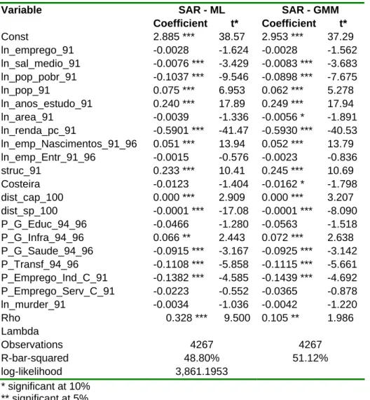
Table 3.D.2 - Estimates for per capita income – SAR SAR - ML SAR - GMM Variable Coefficient t* Coefficient t* Const 2.885 *** 38.57 2.953 *** 37.29 ln_emprego_91 -0.0028 -1.624 -0.0028 -1.562 ln_sal_medio_91 -0.0076 *** -3.429 -0.0083 *** -3.683 ln_pop_pobr_91 -0.1037 *** -9.546 -0.0898 *** -7.675 ln_pop_91 0.075 *** 6.953 0.062 *** 5.278 ln_anos_estudo_91 0.240 *** 17.89 0.249 *** 17.94 ln_area_91 -0.0039 -1.336 -0.0056 * -1.891 ln_renda_pc_91 -0.5901 *** -41.47 -0.5930 *** -40.53 ln_emp_Nascimentos_91_96 0.051 *** 13.94 0.052 *** 13.79 ln_emp_Entr_91_96 -0.0015 -0.576 -0.0023 -0.836 struc_91 0.233 *** 10.41 0.245 *** 10.69 Costeira -0.0123 -1.404 -0.0162 * -1.798 dist_cap_100 0.000 *** 2.909 0.000 *** 3.207 dist_sp_100 -0.0001 *** -17.08 -0.0001 *** -8.090 P_G_Educ_94_96 -0.0466 -1.280 -0.0563 -1.518 P_G_Infra_94_96 0.066 ** 2.443 0.072 *** 2.638 P_G_Saude_94_96 -0.0915 *** -3.167 -0.0925 *** -3.142 P_Transf_94_96 -0.1108 *** -5.858 -0.1115 *** -5.661 P_Emprego_Ind_C_91 -0.1382 *** -4.585 -0.1439 *** -4.692 P_Emprego_Serv_C_91 -0.0223 -0.552 -0.0365 -0.878 ln_murder_91 -0.0034 -1.036 -0.0042 -1.220 Rho 0.328 *** 9.500 0.105 ** 1.986 Lambda Observations 4267 4267 R-bar-squared 48.80% 51.12% log-likelihood 3,861.1953 * significant at 10% ** significant at 5% *** significant at 1%

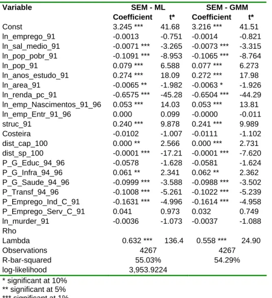
Table 3.D.3 - Estimates for per capita income – SEM SEM - ML SEM - GMM Variable Coefficient t* Coefficient t* Const 3.245 *** 41.68 3.216 *** 41.51 ln_emprego_91 -0.0013 -0.751 -0.0014 -0.821 ln_sal_medio_91 -0.0071 *** -3.265 -0.0073 *** -3.315 ln_pop_pobr_91 -0.1091 *** -8.953 -0.1065 *** -8.764 ln_pop_91 0.079 *** 6.588 0.077 *** 6.273 ln_anos_estudo_91 0.274 *** 18.09 0.272 *** 17.98 ln_area_91 -0.0065 ** -1.982 -0.0063 * -1.926 ln_renda_pc_91 -0.6575 *** -45.28 -0.6504 *** -44.29 ln_emp_Nascimentos_91_96 0.053 *** 14.03 0.053 *** 13.81 ln_emp_Entr_91_96 0.000 0.099 -0.0000 -0.011 struc_91 0.240 *** 9.878 0.241 *** 9.989 Costeira -0.0102 -1.007 -0.0111 -1.102 dist_cap_100 0.000 ** 2.566 0.000 *** 2.731 dist_sp_100 -0.0001 *** -17.21 -0.0001 *** -7.620 P_G_Educ_94_96 -0.0578 -1.628 -0.0581 -1.624 P_G_Infra_94_96 0.061 ** 2.341 0.062 ** 2.362 P_G_Saude_94_96 -0.0999 *** -3.588 -0.0988 *** -3.502 P_Transf_94_96 -0.1008 *** -5.261 -0.1022 *** -5.239 P_Emprego_Ind_C_91 -0.1631 *** -4.996 -0.1614 *** -4.958 P_Emprego_Serv_C_91 0.041 0.973 0.032 0.749 ln_murder_91 -0.0036 -1.073 -0.0037 -1.088 Rho Lambda 0.632 *** 136.4 0.558 *** 24.90 Observations 4267 4267 R-bar-squared 55.03% 54.29% log-likelihood 3,953.9224 * significant at 10% ** significant at 5% *** significant at 1%

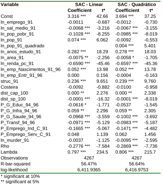
Table 3.D.4 - Estimates for per capita income – SAC

SAC - Linear SAC - Quadrático

Variable Coefficient t* Coefficient t* Const 3.316 *** 42.66 3.694 *** 37.25 ln_emprego_91 -0.0011 -0.687 -0.0012 -0.730 ln_sal_medio_91 -0.0068 *** -3.216 -0.0067 *** -3.155 ln_pop_pobr_91 -0.1028 *** -8.255 -0.0985 *** -8.019 ln_pop_91 0.074 *** 6.062 -0.0092 -0.553 ln_pop_91_quadrado 0.004 *** 5.401 ln_anos_estudo_91 0.282 *** 18.29 0.278 *** 18.03 ln_area_91 -0.0075 ** -2.256 -0.0058 * -1.705 ln_renda_pc_91 -0.6590 *** -45.46 -0.6597 *** -45.36 ln_emp_Nascimentos_91_96 0.052 *** 13.98 0.052 *** 13.78 ln_emp_Entr_91_96 0.000 0.156 -0.0004 -0.163 struc_91 0.236 *** 9.651 0.239 *** 9.760 Costeira -0.0092 -0.882 -0.0100 -0.958 dist_cap_100 0.000 ** 2.276 0.000 ** 2.338 dist_sp_100 -0.0001 *** -16.32 -0.0001 *** -8.019 P_G_Educ_94_96 -0.0616 * -1.771 -0.0537 -1.545 P_G_Infra_94_96 0.059 ** 2.296 0.059 ** 2.305 P_G_Saude_94_96 -0.0968 *** -3.559 -0.1002 *** -3.692 P_Transf_94_96 -0.0971 *** -5.129 -0.0983 *** -5.187 P_Emprego_Ind_C_91 -0.1665 *** -5.067 -0.1471 *** -4.482 P_Emprego_Serv_C_91 0.048 1.139 0.062 1.456 ln_murder_91 -0.0037 -1.125 -0.0095 *** -2.595 Rho -0.2776 *** -7.584 -0.2869 *** -7.736 Lambda 0.797 *** 234.5 0.806 *** 215.7 Observations 4267 4267 R-bar-squared 56.47% 56.64% log-likelihood 6,411.9365 6,416.9753 * significant at 10% ** significant at 5% *** significant at 1%

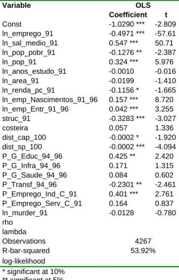
Table 3.D.5 - Estimates for formal employment – OLS OLS Variable Coefficient t Const -1.0290 *** -2.809 ln_emprego_91 -0.4971 *** -57.61 ln_sal_medio_91 0.547 *** 50.71 ln_pop_pobr_91 -0.1276 ** -2.387 ln_pop_91 0.324 *** 5.976 ln_anos_estudo_91 -0.0010 -0.016 ln_area_91 -0.0199 -1.410 ln_renda_pc_91 -0.1156 * -1.665 ln_emp_Nascimentos_91_96 0.157 *** 8.720 ln_emp_Entr_91_96 0.042 *** 3.255 struc_91 -0.3283 *** -3.027 costeira 0.057 1.336 dist_cap_100 -0.0002 * -1.920 dist_sp_100 -0.0002 *** -4.094 P_G_Educ_94_96 0.425 ** 2.420 P_G_Infra_94_96 0.171 1.315 P_G_Saude_94_96 0.084 0.602 P_Transf_94_96 -0.2301 ** -2.461 P_Emprego_Ind_C_91 0.401 *** 2.761 P_Emprego_Serv_C_91 0.164 0.837 ln_murder_91 -0.0128 -0.780 rho lambda Observations 4267 R-bar-squared 53.92% log-likelihood * significant at 10% ** significant at 5% *** significant at 1%