Technology adoption and structural transformation: evidence from the industrialization of the sugarcane sector

(1)

Technology Adoption and Structural Transformation:

Evidence from the Industrialization of the Sugarcane

Sector

Francisco J. M. Costa

*

Francisco Lima

*

June 15, 2020

Abstract

This paper shows how the adoption of an agricultural technology necessary to meet new environmental standards can prompt structural transformation in an emerging economy. We study the fast spread of mechanical harvesting that followed the prohibi-tion of pre-harvest field burning in the sugarcane sector in S˜ao Paulo state, Brazil. We combine remote-sensing data on sugarcane production and censuses data to estimate the impacts of field mechanization on the local labor markets. We find that the adoption of mechanical harvesting led to industrialization of the field; a one standard deviation larger adoption of agricultural mechanization reduces the share of workers employed in the agricultural sector by 2.3 percentage points, and increases the employment share of manufacturing and services sector by 1.7 and 1.1 percentage points, respectively. Keywords: Technology Adoption; Structural Transformation; Labor Market; Environ-mental Regulation; Sugarcane.

JEL Codes: O14, O15, Q16, Q52.

We would like to thank Sam Bazzi, Carlos Eugˆenio Costa, Martin Fiszbein, Jason Garred, Cec´ılia Machado, Romero Rocha, Marcelo Sant’Anna, Edson Severnini and seminar participants at EPGE, NEUDC 2016, Jobs and Development Conference (World Bank), LCM Conference (FEA-USP), PET 16, SBE 2015, 1st REAP Meeting, VII CAEN-EPGE Meeting. We gratefully acknowledges financial support from Rede de Pesquisa Aplicada FGV and CAPES/Brasil (Grant #001).

*_{FGV EPGE Escola Brasileira de Economia e Finan¸}_{cas, Rio de Janeiro, Brazil. E-mails: Costa,}

(2)

1 Introduction

Agricultural mechanization is the process of using machinery to mechanize the work of agriculture, greatly increasing farm worker productivity. It eases and reduces hard labor, improves productivity, and contributes to mitigating climate related hazards. On the other hand, it can displace unskilled farm labor and can cause environmental degradation (such as pollution, deforestation, and soil erosion). Based on the development literature, local productivity gains brought by new technologies may lead to wider and more positive effects to the local economy1_{and reallocate labor toward industry (}_{Bustos et al.}_,₂₀₁₆_;_Carillo_, ₂₀₂₀_),

stimulating the development process.

This paper asks whether agricultural mechanization necessary to meet new environmental standards can prompt structural transformation in an emerging economy. The prohibition of pre-harvest field burning set in motion the widespread adoption of mechanical harvesting in the sugarcane sector in the state of S˜ao Paulo, Brazil. We investigate the effect of the adoption mechanical harvesting on structural transformation – measured by the changes in the sector composition of the local economic activity –, and the distribution of skills employed in each sector. Our results indicate that agricultural mechanization led to local structural transformation and contributed to the industrialization of the agricultural production chain.

Sugarcane is one of the main crops in Brazil and the world’s largest crop by production quantity (Walter et al., 2014).. FAO estimated that sugarcane was cultivated on about 26 million hectares, in more than 90 countries, with a worldwide harvest of 1.83 billion tons in 2012. Sugarcane straw burning during the harvest periodis responsible for a great amount of pollutant gases in atmosphere which cause respiratory diseases in the local population.2

Environmental concerns led S˜ao Paulo – the richest and largest producer state in Brazil – to pass a state law in 2002 outlying the timeline to end sugarcane pre-harvest burning on large properties by 2021 (State Law n° 11,241). In 2007, S˜ao Paulo state and the Organization of Sugarcane Producers (ORPLANA) revised the timeline and set to halt sugarcane pre-harverst burning by 2014.

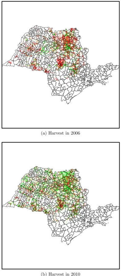
Sugarcane can be harvested using two different technologies: the traditional harvesting, by hand with pre-harvest field burning; and the mechanical harvesting, with no need for burning. Thus, the only way to comply with the new regulation is to adopt the mechanical harvesting. Figure1 shows a map from S˜ao Paulo municipalities with the sugarcane planted

1_{On local effects of productivity shocks in agriculture see} _Matsuyama₍₁₉₉₂_); _{Foster and Rosenzweig}

(2004,2008); Hornbeck(2012);Hornbeck and Naidu(2012); Bustos et al.(2016);Henderson et al.(2015);

Hornbeck and Keskin(2015);Marden(2016).

2₍_{Rangel and Vogl}_,₂₀₁₉_),_{Macedo et al.}₍₂₀₀₈_),_{Can¸cado et al.}₍₂₀₀₆_);_{Dominici et al.}₍₂₀₁₄_);_{Rangel and}

(3)

area colored by harvesting type in 2006 and in 2010. We see that, the area in the state with mechanical harvesting (in green) grew from around 30% in 2006 to 55% in four years.3 _Due

to agricultural mechanization, less workers are needed to harvest the same planted area4_,

it is thus a labor saving technology. We study the effect of such shock on local structural transformation. The mechanical harvest also employs workers with a different set of skills than the the one employed by the traditional harvesting – e.g. machine operators, mechanics, and engineers(Moraes, 2007) – , it is thus a skill biased technical change. We investigate whether this shock affected the distribution of skills employed in each sector.

We exploit this fast adoption of agricultural mechanization, and estimate its medium-run impact on local labor market structure. To this goal, we use four main datasets: population census; input-output tables; remote sensing data of sugarcane planting and harvesting (CANASAT-INPE), and, GIS-based geomorphometric data (TOPODATA). We use the remote sensing data to create an index for the adoption of mechanical harvesting in each plot of land with sugarcane production. In order to characterize the evolution of mechanization by municipality, we create an Adoption Index measuring the fraction of the area of sugarcane fields with mechanical harvesting in 2010 relative to the baseline fraction of mechanical harvesting. We pair this index with labor market data across sectors at the municipality level, for 2000 and 2010.

In order to unveil the causal effects of agricultural mechanization on the evolution of labor market outcomes, we use the land slope of the pixels with sugarcane production as an instrument for the adoption of harvest mechanization. The reason for this instrument comes from engineering constraints: it is more costly to introduce mechanical harvesting in steeper plots of land.5 _{Our identifying assumption is that, conditional on a series of covariates,land}

slope of pixels with sugarcane production do not affect the evolution of labor market outcomes directly, but only indirectly via agricultural mechanization.

We find that a one standard deviation larger adoption of agricultural mechanization reduces the share of workers employed in the agricultural sector by 2.3 percentage points, and

3_{The first statistic of mechanical harvest we could find is}_{ALCOOBR ´}_AS₍₂₀₀₃_{), which states that around}

15 percent of the sugarcane harvested in S˜ao Paulo in 2003 used mechanical harvesting with no pre-harvest burning.

4_{According to some estimates from the industry (}_SGPR_,₂₀₀₉_{), one harvest machine can substitute around}

eighty hand workers.

5_{Braunbeck and Magalh˜}_aes ₍₂₀₁₀_{) argues that because of soil irregularities and driving conditions it is}

difficult to use a combine in areas with slope greater than 12 percent. However, advances in the off-road vehicle engineering, such as four wheel drive, helped to mechanize areas with a slope up to 18 percent. In fact, the state law from 2002 set different goals and deadlines for areas steeper than 12 degrees. This distinction was dropped in the 2007 protocol deal. In Appendix B, we use a regression discontinuity design to estimate if there were any discontinuous adoption of mechanical harvesting at the 12 degree cut-off. We find no local difference in adoption at the cut-off.

(4)

increases the employment share of manufacturing and services sector by 1.7 and 1.1 percentage points, respectively. We interpret these findings as evidence that agricultural mechanization led to local structural transformation. We find that this employment reallocation happened mostly among unskilled workers. In particular, we document that adoption of mechanical harvest changed the labor composition in agricultural sector by increasing the share of skilled-unskilled workers ratio. We find no effect on the composition of skills in the manufacturing and services sector.

Last, we study a potential mechanism through which the agricultural mechanization created structural transformation. Bustos et al. (2016) argue that in a small open economy, a labor saving technical change releases labor force previously employed in the agricultural sector which are then absorbed by the manufacturing and services sectors. On the other hand, mechanization, by increasing the productivity in the downstream sector, may also particularly benefit manufacturing and services industries in the agricultural production chain. We use input-output tables to assess this channel and estimate heterogeneous effects of adoption of mechanical harvesting onindustries linked and non-linked to the agricultural sector using input-output tables. Our results indicate that the increase in employment share of manufacturing and services sectors is restricted to industries linked to the sugarcane sector. We find that a one standard deviation larger adoption of agricultural mechanization increases the employment share of manufacturing and services industries linked to the agricultural sector by 1.9 percentage points, and 0.9 percentage point, respectively. We interpret this as evidence that agricultural mechanization contributed to the industrialization of the agricultural production chain in these areas.6

This paper primarily contributes to the literature that studies the implications of technolog-ical progress in agriculture on development and industrialization. In our context, technology adoption represented a shock to agriculture productivity with impacts on local development (Foster and Rosenzweig, 2004,2008; Hornbeck, 2012; Hornbeck and Naidu, 2012; Henderson et al., 2015; Hornbeck and Keskin, 2015; Marden, 2016; Carillo,2020) and structural trans-formation. Matsuyama (1992) shows that for small open economies facing perfectly elastic demand for agricultural and manufacturing goods, a Hicks-neutral increase in agricultural productivity reduces the industrial sector by reallocating labor towards agriculture. This model has only one production factor: labor. Bustos et al. (2016) extended this model to two production factors: land and labor. In this case, technical change can be factor-biased. When technical change in agriculture is strongly labor saving, an increase in agricultural productivity

6_Assun¸_c˜_{ao et al.}₍₂₀₁₆_{) shows evidence from a different Brazilian state that the introduction of sugarcane}

mills increases the conversion of pasture to sugarcane land. Together with our results, this is evidence of complementarity between agricultural and manufacturing industries within the sugarcane production chain.

(5)

leads to manufacturing and services growth as it increases residual labor supply and local income. Bustos et al. (2016) provide empirical evidence on the impacts of the adoption of genetically engineered soybean seeds (a labor saving technology change) on the industrial sector in Brazil. Differently from this paper, we study a skill-biased technical change (Autor et al., 2003;Carillo,2020) and find that the agricultural mechanization increases the size of manufacturing and services sectors, and this effect was focused on industries connected to the agricultural sector.

We also contribute to the literature on effects of environmental regulation on local labor markets and economic competitiveness. Most of the papers find that environmental regulation in the United States harm manufacturing firms and workers (Berman and Bui,2001;

Greenstone, 2002;Deschenes, 2011; Walker, 2011; Kahn and Mansur,2013). Walker (2013) argue that the regulatory costs should be measured by the costs associated to reallocating production across industries because most of its effects pertain to the distribution of economic activity across sectors, not levels. Closer to this paper,Harrison et al.(2015) andTanaka et al.

(2014) study the effects of environmental regulation on the productivity of manufacturing firms India and China, respectively. These papers tell a different story from the papers on developed economies. They find that environmental regulation improves firms productivity by increasing investments in new technologies or by affecting firms’ dynamics.7 Our main contribution to this literature is to investigate a potentially wider benefits of environmental regulation in an emerging country context. In the developing world, reallocation of workers across sectors – in particular moving workers out of the traditional low productivity agriculture sector – may be beneficial to the local economy. In the episode we study, local economies benefit with the adoption of a technology that was previously available. A lot of attention has been drawn to understanding the determinants of technology adoption in non-developed countries (Esther Duflo and Robinson, 2006; Conley and Udry,2010; Bandiera and Rasul, 2006). The literature review in Foster and Rosenzweig (2010) shows that the perceived profitability and benefits brought by the technology are key for adoption. Social learning, networks, biased believes or fixed costs have been shown to be important mechanisms that prevent desirable technologies from being adopted. In our case, environmental regulation aimed at reducing the level of pollutant gases, may have induced the adoption of an improved technology which was not privately valued initially, but that, at scale, may produce meaningful productivity gains to the economy. Therefore, our paper contributes more broadly to the literature on the consequences of technology adoption on local development (Berman et al., 1998; Beaudry

7_{As argued by} _{Harrison et al.} ₍₂₀₁₅_{), these are supportive evidence for a weak version of the Porter}

Hypothesis, where environmental regulation does not trigger innovations or R&D, but technological catch up or firm selection.

(6)

et al., 2006).

The remaining of the paper is organized as follows. Section 2 provides background information. Section 3 describes the data. Section 4 presents our empirical strategy. Section 5 shows the results. Section 6 presents some robustness checks. And, section 7 concludes.

2 Background

In this section, we discuss the sugarcane industry in the state of S˜ao Paulo with a greater focus on the two aspects most relevant to the paper: harvesting technology and labor markets. According to the Food and Agriculture Organization (FAO), in 2012, sugarcane was cultivated on about 26 million hectares across more than 90 countries, with a worldwide harvest of 1.83 billion tons. Brazil is the top producer in the world by production quantity (Walter et al.,

2014), being responsible for more then a third of worldwide production. According to the Brazilian Sugarcane Industry Union (UNICA), S˜ao Paulo is responsible for more than two thirds of Brazilian production, and it would be the second largest world producer.

Harvesting technologies. Sugarcane is a semi-perennial crop, with the harvesting season in S˜ao Paulo state going from April to December. Sugarcane can be harvested using two broad technologies: the traditional harvesting, using pre-harvest field burning and manual workers armed with knifes; and the mechanical harvesting, using a combine harvester without field burning. In the traditional harvesting, pre-harvest field burning is used to clean the field in preparation for the manual workers, as the fire cleans the area from straws and other weeds, as well as chase away any dangerous animals. The sugarcane straw burning is responsible for a great amount of pollutant gases in the atmosphere (Macedo et al., 2008), being responsible for several respiratory diseases in the local population (Rangel and Vogl, 2019)(Can¸cado et al., 2006; Dominici et al., 2014; Rangel and Vogl, 2015). Other environmental problems related to sugarcane straw burning are soil and groundwater contamination (SGPR, 2009). Also, traditional harvesting in Brazil is characterized by mostly unskilled and temporary job positions.

On the other hand, mechanical harvesting uses modern harvesters and can be made without field burning, as the combine processes the straws. By avoiding straw burning, this technology is substantially less pollutant than the traditional harvesting. It is a capital-intensive technology that shows returns to scale. According to some estimates from the industry (SGPR, 2009), one harvest machine can substitute around eighty hand workers. Despite the productivity gains of mechanization, the availability of low wages unskilled and seasonal workers make the traditional harvesting technology attractive for sugarcane

(7)

producers relative to labor saving capital investments. Furthermore, mechanical harvesting requires a set of skilled workers (e.g., machine operators, and mechanics) which are scarce in many rural areas (Moraes, 2007). There are also natural constraints to the adoption of mechanical harvesting, in particular the cost of mechanization depends on the slope of the land – it is cheaper to mechanize the harvest in flatter terrains.

State plan to halt pre-harverst burning. In 2002, with the goal of reducing respiratory diseases and climate change impacts, the state of S˜ao Paulo passed a law outlying a timeline to end sugarcane pre-harvest burning by 2021.8 This involved a progressive substitution of traditional harvesting by mechanical harvesting, since the prohibition of pre-harvest burning reduces the productivity of traditional harvesting , as fire is the cheapest way to clean the field (Novaes et al., 2007). In 2006, the regulation was further strengthened when the state government and the Organization of Sugarcane Producers (ORPLANA) sealed a Cooperation Protocol shortening the deadline to halt burning by 2014. This protocol also created an agro-environmental certificate for clean sugarcane.

Figure 1 shows a map of S˜ao Paulo municipalities color-coding areas with sugarcane production by harvesting type in 2006 and 2010 – red pixels are plots of land with pre-harvest burning and green pixels use mechanical harvesting. As we can see in the maps, sugarcane production is distributed across the state of S˜ao Paulo and the share mechanical harvesting almost doubled in the four years following the the signature of the protocol, from 30% in 2006 to 55% in 2010.

Local labor markets. The main sectors in sugarcane producing municipalities are agriculture and services, each employing together around 40% of the labor force , the manufacturing sector employ 10% of the labor force. Most of the labor force is unskilled, only 30% holds at least a high school degree. This figure is even lower in the agricultural sector, where only 20% of the permanent (non-seasonal) workers hold a high school degree. The sugarcane sector has a bad record in terms of workers’ conditions and environmental compliance. There are several reports about criminal recruitment and over-exploitation of labor, as well as precarious accommodation, high level of workplace accident, death by exhaustion, and child labor (SGPR,2009). In the sugarcane industry, especially in farms using traditional harvesting, the largest share of workers were unskilled and seasonally employed. Over the last decades, however, with the expansion of mechanical harvesting, the sugarcane industry started training and recruiting more skilled workers, such as machine operators, mechanics, and engineers(Moraes, 2007). In 2009, UNICA, the Federal Government and the

(8)

National Confederation of Agricultural Workers (CONTAG) signed the National Agreement to Improve Sugarcane Working Conditions. The aim of this Agreement was to improve better labor practices and to promote the reintegration of workers who lost their jobs due to the advance of mechanization.

Thus, environmental and labor regulations may have contributed to the expansion of mechanical harvesting. This can affect labor demand in these regions through two channels. First, less workers are needed to harvest the same planted area: labor saving technologies may lead to structural transformation (Bustos et al., 2016). Second, this is a skill biased technical change increasing the demand for skilled worker relative to unskilled workers in the agricultural sector, and consequently in the local economy.

3 Data

The main data sources are: population census; input-output tables; remote sensing data of sugarcane planting and harvesting (CANASAT-INPE); and, GIS-based geomorphometric data (TOPODATA).

Labor market data. We draw labor market data from the Brazilian Demographic Census, which is produced by the Brazilian Institute of Geography and Statistics (IBGE) every ten year.9 We use the last three rounds of the survey (1991, 2000 and 2010). This allows us to observe the variables of interest before and after the environmental regulation is passed, as well as to conduct robustness checks and study pre trends. We restrict our analysis to working-age population, defined as all individuals between 18 and 60 years old. The variables we focus on are the sector in which the individual was working during the previous week10 _ans

its education level. We define an individual as skilled if it holds at least a high school degree, and as unskilled otherwise.11 _{For each municipality, we compute employment shares as the}

numbers of workers in each sector divided by working age population. We also compute unskilled employment shares.

To characterize industries as linked and non-linked to the agricultural sector, we use Brazilian input-output tables for the year of 2000 produced by IBGE. The data classifies 55

9_{The main advantage of this data relative official registries is that it is has a comprehensive coverage of}

rural areas and informality. This is key as informality is large in the agriculture sector.

10_{We identify the sector an individual was employed in the previous week as declared in the census}

(classification CNAE 1.0). We classify the market in three sectors using 2 digits CNAE 1.0: agricultural sector (codes from 01 to 05), manufacturing sector (codes from 15 to 37), and services sector (codes from 40 to 74 and 80 to 94).

(9)

industries which we merge with the census data using CNAE 1.0 classification12_{. We follow}

(Allcott and Keniston, 2018) to define an industry as linked if the share of output purchased by the agricultural sector is larger than 0.1 percent or if the agricultural input cost share is larger than 0.1 percent; an industry is classified non-linked otherwise.

Production and harvest data. We use granular remote sensing data for sugarcane production in S˜ao Paulo State from CANASAT, produced by the National Institute For Space Research (INPE). It contains two different sets of images: annual sugarcane planted area from 2003 to 2013, CANASAT-Planted Area; and annual sugarcane harvesting from 2006 to 2012, CANASAT-Harvest. CANASAT-Harvest was created to support the implementation of the Cooperation Protocol signed in 2006, and identifies traditional sugarcane harvesting (with pre-harvest burning) and mechanical harvesting (no pre-harvest burning) (Rudorff et al., 2010a; Adami et al., 2012). 13 _{We are unable to extend the analysis to other states}

because CANASAT-Harvest covers only S˜ao Paulo state.14

We aggregate the remote sensing data at the municipality level to merge with labor market data from census. For each municipality we compute the number of pixels of each harvesting type and the number of pixels with planted area. Our sample consists of the 393 municipalities in which we observe sugarcane cropping. For each of these municipalities, we construct a measure of technology adoption, Mechanization Index, defined as the fraction of the area with mechanical harvesting out of the total area planted with sugarcane in the baseline.

Land characteristics. We calculate the slope of each pixel using high-resolution digital topographic data from TOPODATA.15 _{This data has resolution of one arcsecond,}

approx-imately 9.49 hectares. We overlay TOPODATA and CANASAT to get the land slope of the pixels with sugarcane production. That is, we calculate the land slope of each plot of land actually producing sugarcane in S˜ao Paulo. We, then, calculate the share of sugarcane planted area in land slope bins for each municipality.

12_{This classification merges 55 industries from input-output tables with 147 industries using 4 digits CNAE}

1.0 classification which we aggregate at 2 digits CNAE 1.0. When a 2 digits industry is classified as linked and non-linked we consider it as linked only.

13_{This classification is done using visual interpretation technique of remote sensing images, obtained}

between April and December in each crop year. Most of the sugarcane harvesting is performed during the dry season, when it is relatively favorable to acquire cloud free images. Identification of harvest type is based on the reflectance difference between mechanical harvesting and pre-harvest burning fields (Aguiar et al.,2011a).

14_{Rudorff et al.}₍_2010b_{) and}_{Aguiar et al.}₍_2011b_{) describe the specifics for CANASAT planted area and}

harvest, respectively.

15_{Land slope is based on the Digital Elevation Model (MDE) and the original data is from the Shuttle}

(10)

We measure land suitability for technological change in agriculture by using estimates of potential sugarcane yields from the FAO-GAEZ database. This data calculates potential yields under different scenarios of technology use.16 _{Following (}_{Bustos et al.}_, ₂₀₁₆_{), we}

construct a measure of suitability for technical change in sugarcane for each municipality by deducting the average potential yield under low inputs from the average potential yield under high inputs. Last, as a measure of market access, we calculate the distance from each plot of land with sugarcane to roads using the GIS road maps from the Ministry of Transportation. We calculate the average distance of sugarcane pixels to roads for each municipality.

4 Empirical Strategy

In this section we describe our empirical strategy. We first define the measure of adoption of mechanical harvesting. We then present our main regression specification and discuss potential identification issues. Last, we propose an instrumental variable strategy to overcome these issues.

4.1 Agricultural mechanization index

We start by creating our agricultural mechanization index to capture the degree of me-chanical harvesting in sugarcane plantations. This index consists in the share of sugarcane planted area (number of pixels) with mechanical harvesting in a municipality j in year t: M echanizationjt ≡ mij/ajt where mjt is the area (number of pixels) with mechanical

harvesting, and ajt is the total area (number of pixels) with sugarcane in municipality j and

year t.

Our main variable of interest is the adoption of agricultural mechanization between 2000 and 2010:

AdoptionIndexj ≡ M echanizationj,2010− M echanizationj,2000. (1)

As discussed before, we do not observe sugarcane planted area for 2000, so we consider 2003 planted area as the baseline planted area at 2000.17 _{Likewise, there is no georeferenced data}

on harvesting type for 2000. Thus, in our main specification we assume there is no mechanical harvesting in 2000.18

16_{Yields under the low technology are described as those obtained planting traditional seeds, with no use}

of chemicals nor mechanization. Yields under the high technology are obtained using improved high yielding varieties, optimum application of fertilizers and herbicides, and mechanization.

17_{CANASAT-Planted Area covers sugarcane planted area from 2003 to 2013 in Brazil.}

(11)

4.2 Main Specification

Our empirical strategy relies on the assumption that goods can be traded across municipalities but labor markets are local. We investigate whether agricultural mechanization – a labor saving technology – lead to structural transformation as measured by changes in the composition of local economic activity.More specifically, our main goal is to estimate the impacts of technology adoption in the agricultural sector on local labor markets variables. We evaluate the evolution of these labor market outcomes between 2000 and 2010, ∆Yj ≡ Yj,2010− Yj,2000,

in order to capture a medium-run effect of mechanization. Our main regression equation is: ∆Yj = α + βAdoptionIndexj + γXj + νj (2)

where Xj is a vector of municipality level controls. All our regressions include a set of

controls: the share of rural population in 2000, the log of labor force in 2000, and the the log of sugarcane planted area in 2003 to allow for differential trends for municipalities with different initial urbanization rates, size, and initial sugarcane production, respectively. A further concern about identification is that the initial presence of skilled labor may foster technology adoption and influence labor market, as pointed by Beaudry et al. (2006), thus we control for the share of illiterates and of skilled workers in 2000. Because higher baseline education levels in the region may facilitate technology adoption and dynamic,. We control for population density in 2000 to account for differences inurbanization intensity and labor market integration. We also add a control for distance to roads to allow different initial trade costs. We add controls for soil suitability using the same measure defined in (Bustos et al.,

2016) to control for differential trends by potential sugarcane yield under high inputs versus low inputs.

The coefficient of interest is β which captures the effect of adoption of agricultural mechanization in the sugarcane sector on the evolution of different labor market outcomes ∆Yj. Tables ?? and ?? report summary statistics of our explanatory and dependent variables,

respectively. νj is the idiosyncratic error term. We follow (Bustos et al., 2016) and estimate

heteroskedasticity-robust standard error estimators.

Reduced form estimates of the equation above may have identification issues if there is any endogeneity between labor market development and the adoption of the technology in the field. For example, consider a labor market shock that increases wages at a level that producers opt to pay the fixed costs of adopting a new technology. Alternatively, consider for example local shocks to the agricultural sector – e.g., local government subsidizing sugarcane industry –, which affects directly both technology adoption and labor market outcomes. In these cases, ordinary least square estimates would be biased and one would not unveil the

(12)

causal relation of the adoption of agricultural mechanization. Next, we propose a strategy to overcome this issue.

4.3 Instrumental Variable

We propose to identify the causal effect of the technology adoption on structural transformation by using a instrumental variable strategy. We use land slope of sugarcane planted area as an instrument for the adoption of mechanical harvesting in the sugarcane industry. The intuition for using this instrument is that it is more costly to mechanize steep areas (Moraes,

2007), so producers with land in steep terrains would resist more to adopt the mechanical harvesting technology.

Our estimates using land slope as an instrument for the adoption of mechanical technology capture the causal relation between technology adoption and labor market outcomes if: (i) slope is correlated to adoption of mechanization; and (ii) slope is uncorrelated to the error term νj in equation 2 . In words, slope must be correlated with the adoption of mechanical

harvesting in the sugarcane industry, and must have no direct influence on the evolution of labor market outcomes except via the mechanical harvesting adoption. To shed light on assumption (ii), we assess whether producers prefer to expand sugarcane production to flatter terrains. If these terrains represented a better opportunity for the extensive margin of sugarcane areas, we would observe a negative relation between expansion of sugarcane production and land slope, as producers would be gradually moving towards worst – steeper – terrains. We analyze a panel data of sugarcane planted area for S˜ao Paulo state from 2003 to 2013. FigureA4 plots the expansion of planted areas since 2003 by different land slopes. We can see that the growth of planted areas – i.e., the planted area in year t divided by planted area in 2003 – is relatively homogeneous across slope levels. We observe that the increase in total planted area does not seem to be concentrated in terrains with certain slopes. This give us some reassurance that our instrument is not related with an underlying factor determining the expansion of the sugarcane industry in these municipalities.

Our first stage regression equation is:

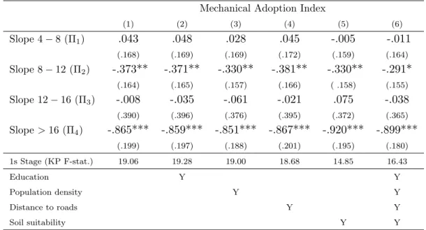
AdoptionIndexj = Π1Slope4−8j + Π2Slope8−12j + Π3Slope12−16j + Π4Slope16j + λXj + εj (3)

where Xj is a vector of controls, and Slopei−i 0

is the share of sugarcane planted area – i.e., pixels with sugarcane production – in municipality j with slope in the interval [i, i0) and Slope16 _{is the share of sugarcane planted area with slope greater than 16. That is, we only}

(13)

category is the share of land with sugarcane planted in slopes between 0 and 4 degrees.19

Table 3 presents the first stage results. The signs of the coefficients are consistent with our intuition, we find a negative relation between slope and agricultural mechanization robust to all our different controls. Our instrument has sufficient explanatory power, the Kleibergen-Paap F statistic (Kleibergen and Paap, 2006) is 19.06 with standard controls and 16.43 in the specification with all additional controls.

5 Results

In this section, we estimate the effects of agricultural mechanization on local structural transformation in S˜ao Paulo state, as measured by a change in the industry composition of local economies.

5.1 Industry composition

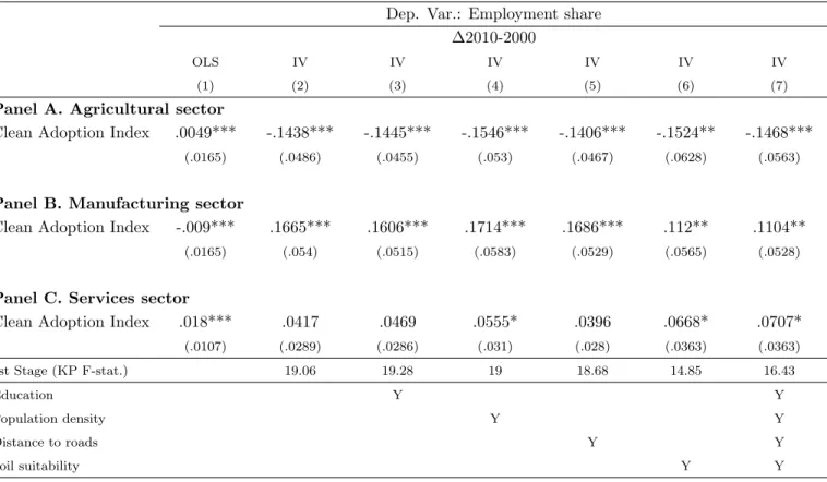
Table 4 presents the estimated effects of agricultural mechanization on employment share by sector – agricultural, manufacturing, and services.20 _{The dependent variable in Panel A is}

the share of permanent workers employed in the agricultural sector. The OLS estimates, in column 1, suggests that the agricultural sector grew faster in regions with greater adoption of mechanical harvest. This relationship is likely biased as there may be other factors inducing the growth of this sector and technology adoption. Columns 2 to 7 present the 2SLS results using the slope of sugarcane field as an instrument for adoption of mechanical harvest. We find that the instrumental variables estimates indicates that agricultural mechanization led to a faster reduction in the agricultural employment share between 2000 and 2010. Point estimates are very stable and remains statistically significant when we add a series of controls for baseline education levels (column 3), population density (column 4), distance to roads (column 5), and soil suitability for sugarcane (column 6) as we discussed in the previous section. Column 7 presents our preferred specification including the full set of controls. The point estimate of -0.1468 implies that an increase of one standard deviation in Adoption Index (0.154) reduced in 2.26 percentage points the agricultural employment share [0.1468 x 0.154]. This corresponds to approximately 62% of the average reduction in agricultural employment share between 2000 and 2010 [2.26/3.64 ˜ 62%]. Put another way, the agricultural

19_{Notice that slope does not change between years, so we assume that producers do not invest to change the}

terrain, like terrace for example. Terrace is a a very expensive activity so, even if producers would consider doing such investment to the land, this would consist a differential cost of adopting mechanical harvesting.

20_{All regressions are controlled for the share of rural population in 2000, the log of labor force in 2000, and}

(14)

employment share reduced 2.26 percentage points in a municipality that increased agricultural mechanization in one standard deviation (15.4%).

Panel B of table 4 reports a positive and significant coefficient for manufacturing employ-ment share. The point estimate of 0.1104 implies that an increase of one standard deviation in Adoption Index increased manufacturing employment share by 1.70 percentage points between 2000 and 2010, and this corresponds to 37% of the average increase in agricultural employment share. Panel C of the same table reports the coefficient for services employment share. We find a positive coefficient which significance depends on controls. In column 6, our preferred specification, the point estimate of 0.0707 implies that an increase of one standard deviation in Adoption Index increased services employment share by 1.09 percentage points between 2000 and 2010, corresponding to 34.9% of the average increase for this variable.

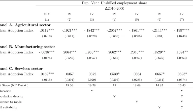
In order to check what type of worker the agricultural sector is releasing we estimate the impacts of agricultural mechanization on unskilled employment share.21 _Table ₅_{presents the}

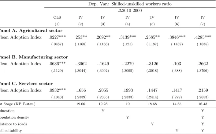
results for unskilled employment share. We find negative and significant results for agricultural unskilled employment share, and positive and significant results for both manufacturing and services sector. The estimates in column 6 imply that a one standard deviation in agricultural mechanization led to a reduction in 3.08 percentage points in agricultural unskilled employment share between 2000 and 2010, this corresponds to 111% of the average reduction in this variable. The impact of a one standard deviation in Adoption Index was of 2.15 and 1.07 percentage points in manufacturing and services sector, respectively.Table 6 presents the results for skilled-unskilled workers ratio. Panel A estimates suggest that agricultural mechanization increased skilled-unskilled in agricultural sector. The point estimate of 0.4285 implies that an increase of one standard deviation in mechanization increased in 6.60 percentage points in skilled-unskilled ratio in agricultural sector, which corresponds to a 51.6% of the average increase of this variable between 2000 and 2010. The IV estimates in Panels B and C are also positive although not significant for both manufacturing and services sector.

To sum up, the results presented in tables 4, 6, and 5 suggest that agricultural mecha-nization – a labor-saving and skill biased technical change – led to structural transformation through a reduction of employment share in agricultural sector and an increase in the employment share of manufacturing and services sector. And more, it seems that this em-ployment reallocation is mostly happening among unskilled workers which also affects the labor composition in agricultural sector.

21_{We computeunskilled employment share as the number of unskilled employed workers in a sector divided}

(15)

5.2 Connected industries

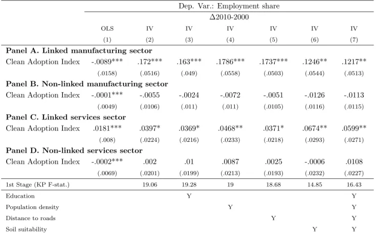
To continue our analysis we investigate which industrial and services sectors are benefiting from the reduction of the share of agricultural employment. (Bustos et al., 2016) shows that a introduction of labor-saving technologies in agriculture can foster structural transformation by releasing workers who find occupation in other sectors. If the structural transformation is driven simply by such labor market channel, all manufacturing industries could stand to benefit from it. On the other hand, manufacturing industries in the agricultural production chain may stand to benefit not only by the labor market channel, but by the improved productivity of the – downstream – agricultural sector. To assess whether services and manufacturing sectors connected to the agricultural sector proportionally benefit from the agricultural mechanization, we estimate the impacts of agricultural mechanization on agricultural and services sector employment shares differentiating between linked and non-linked to the agricultural sector. Table7reports the results for employment share for manufacturing and services industries linked and non-linked to the agricultural sector – we provide greater detail on this classification in Section 3. We find a positive and significant point estimate in Panel A and C, which means that agricultural mechanization led to an increase in employment share for both manufacturing and services industries linked to the agricultural sector. The point estimate of column 7 in Panel A imply that a one standard deviation in agricultural mechanization led to an increase in 1.87 percentage points between 2000 and 2010 in the employment share of manufacturing industries linked to the agricultural sector, which corresponds to 41.7% of the average increase in this variable. The point estimate of column 7 in Panel C implies a 0.92 percentage point increase in the employment share of services industries linked to the agricultural sector due to a one standard deviation in Adoption Index, corresponding to 56.2% of the variation in employment share between 2000 and 2010. We find no effect of adoption of mechanical harvesting on the employment share of manufacturing and services industries not linked to the agricultural sectors. Point estimates in Panels B and D are substantially smaller than the ones in Panels A and C, and are not statistically significant at the usual levels.

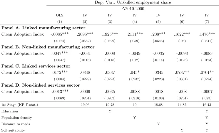
We check what type of workers the other sectors are hiring.Table 8presents the results for unskilled employment share for linked and non-linked sectors. We find positive and significant point estimates for both linked sectors, manufacturing and services, and no significant estimates for non-linked sectors. The point estimates of column 7 in Panel A imply that one standard deviation in our measure of agricultural mechanization led to an increase of 2.27 points in unskilled employment share between 2000 and 2010 for linked manufacturing sectors, corresponding to 55.8% of the average increase in this variable between 2000 and 2010. In Panel C, we find a positive coefficient which significance depends on controls for

(16)

unskilled employment share for linked services sector. The point estimate of column 7 implies a 1.08 percentage point increase in the unskilled employment share due to a one standard deviation of Adoption Index. And, we find no effect on the unskilled employment share of manufacturing and services industries not linked to the agricultural sectors. Point estimates in Panels B and D are negative and substantially smaller than the ones in Panels A and C, and are not statistically significant.

Taken together, our results indicate that the increase in employment share of manufacturing and services sectors was focused on industries linked to the sugarcane sector. We interpret this as evidence that agricultural mechanization contributed to the industrialization of the agricultural production chain. In other words, structural transformation in these areas seem to be have developed through the industrialization of the agriculture sector.

6 Robustness Checks

6.1 Preexisting Trends

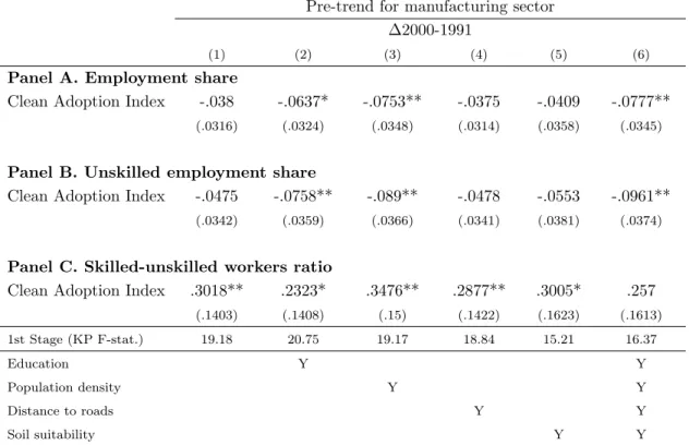
A potential concern of our estimates is that the economy of municipalities better suited for adopting agricultural mechanization could have been already following a different development path, for example already undergoing a structural transformation. We assess whether our results are driven by preexisting trends in the manufacturing sector by estimating equation(2) using as the dependent variable the evolution of labor outcomes in the manufacturing sector from 1991 and 2000. We perform this test for the level manufacturing sector but not for the agricultural and service sectors because there were important changes in the definition of employment after the 1991 census, thus employment variables can not be measured in a consistent way across the 1991 and 2000 censuses for agricultural and services sectors.22

Table A.1 reports the results on pre-trends on employment in the manufacturing sector.23 We find that the manufacturing sector shrank more in areas that came to adopt mechanical harvest in the following decade. The manufacturing secotr in Brazil was particularly harmed by the trade liberalization in the 1990s (Dix-Carneiro and Kovak, 2019). The adoption of mechanical harvest seem to have contributed to revert the deindustrialization process in these

22_{IBGE changed the reference period for employment: in 1991 a person was considered as employed if she}

has worked in the last 12 months, while in 2000 it only included the reference week of the census. This new rule implied that workers performing temporary and seasonal activities who were not employed during the reference week were counted in the 1991 census but not in the 2000 census. This is particularly problematic for the agricultural sector. Also, in 1991 zero-income workers, which are more common in agriculture than in other sectors, were only partially included as workers.

23_{The number of observations is different because new municipalities were created during the 1990s. We}

(17)

regions.

6.2 Migration

Part of our results could be driven by technology adoption affecting migration patterns across municipalities. If this was the case, results could be driven by reallocation of workers across space rather than sectors (Imbert et al.,2018). We investigate this issue by estimating the effect of agricultural mechanization on migration patterns. To do so, we measure net migration rate as the share of the difference between immigrants – working-age individuals that arrived to the municipality on the last 5 years – and outmigrants – working age individuals that left the municipality on the last five years – as a share of workforce five years earlier.24

TableA.2 reports the results. We find no significant evidence that adoption of mechanical harvesting affected net migration between 200 and 2010.

6.3 Different Educational Levels

In our main specification, we classify skilled workers as those holding a high school degree. We check if our results are robust to the classification of skilled and unskilled workers by using two different classifications. In Tables A.3 andA.4 we classify skilled workers as one holding a college degree. In Tables A.5 and A.6 we classify skilled worker as as someone holding a middle school degree. Our main results seem to be robust to our classification of skilled workers, since the point estimates have the same sign and similar magnitude as the ones presented in the previous section.

6.4 Linked industries classification

In our main specification we follow (Allcott and Keniston, 2018) to define an industry as linked if the share of output purchased by the agricultural sector is larger than 0.1% or if the agricultural input cost share is larger than 0.1% – an industry is classified non-linked otherwise. The idea for using such small cutoff values in defining upstream and downstream is conservative in the sense that “non-linked” industries have very limited linkage to agricultural sector and thus should not be directly affected by that sector. A possible concern is that such conservative definition underestimates the impacts on non-linked sector.We address this concern by showing results when we use a cutoff 10 times larger, effectively reducing the possibility for an industry to be linked to the agricultural sector. That is, as robustness, we

24_{Note that we only observe permanent migration. There is no comprehensive and reliable data on seasonal}

(18)

classify an industry as linked if the share of output purchased by the agricultural sector is larger than 1% or if the agricultural input cost share is larger is larger than 1%.

Tables A.7, ?? and A.8 report the estimates for this new linkage classification. We still observe that the employment shares for linked industries in the manufacturing sector grew more in municipalities with greater agricultural mechanization and we find no significant effects on non-linked manufacturing industries. The results for services sector lose significance in this alternative specification. In sum, our findings suggest that agricultural mechanization led to industrialization of the agricultural productive chain, we see that adoption of mechanical harvesting increased employment shares in manufacturing industries linked to agriculture, but no statistical significant effect on non-linked industries. We find weaker evidence that services sectors industries linked to agriculture stood to gain from agricultural mechanization.

7 Conclusion

This paper estimates the causal effects of agricultural mechanization necessary to meet with new environmental regulations on the local labor markets of rural economies within a large emerging country, Brazil. Our identification strategy exploits the fast adoption of mechanical harvesting instrumented with differential adoption costs related to topographic characteristics. We find evidence that agricultural mechanization triggered structural transformation in rural economies.

We find that agricultural mechanization led to industrialization of the agricultural pro-ductive chain, we see that adoption of mechanical harvesting increased employment shares in manufacturing industries linked to agriculture, but no statistical significant effect on non-linked industries. We find weaker evidence that services sectors industries linked to agriculture stood to gain from agricultural mechanization.

References

Adami, M., M. P. Mello, D. A. Aguiar, B. F. T. Rudorff, and A. F. d. Souza (2012). A web platform development to perform thematic accuracy assessment of sugarcane mapping in south-central brazil. Remote sensing 4 (10), 3201–3214. 3

Aguiar, D. A., B. F. T. Rudorff, W. F. Silva, M. Adami, and M. P. Mello (2011a). Remote sensing images in support of environmental protocol: Monitoring the sugarcane harvest in s˜ao paulo state, brazil. Remote Sensing 3 (12), 2682–2703. 13

(19)

Aguiar, D. A., B. F. T. Rudorff, W. F. Silva, M. Adami, and M. P. Mello (2011b). Remote sensing images in support of environmental protocol: Monitoring the sugarcane harvest in s˜ao paulo state, brazil. Remote Sensing 3 (12), 2682–2703. 14

ALCOOBR ÁS (2003). Uma safra recorde. Alcoobrás São Paulo (82), 62–64. 3

Allcott, H. and D. Keniston (2018). Dutch Disease or Agglomeration? The Local Economic Effects of Natural Resource Booms in Modern America. Review of Economic Studies 85 (2), 695–731. 3, 6.4

Assun¸c˜ao, J., B. Pietracci, and P. Souza (2016). Fueling development: sugarcane expansion impacts in brazil. Climate Policy Initiative, Iniciativa para o Uso da Terra (INPUT). 6

Autor, D., F. Levy, and R. Murnane (2003). The skill content of recent technological change: An empirical exploration. Quarterly Journal of Economics. 1

Bandiera, O. and I. Rasul (2006). Social Networks and Technology Adoption in Northern Mozambique. The Economic Journal 116 (514), 896–902. 1

Beaudry, P., M. Doms, and E. Lewis (2006). Endogenous skill bias in technology adoption: city-level evidence from the IT revolution. Technical Report w12521, National Bureau of Economic Research. 1, 4.2

Berman, E., J. Bound, and S. Machin (1998). Implications Of Skill-Biased Technological Change: International Evidence. The Quarterly Journal of Economics 113 (4), 1245–1279.

1

Berman, E. and L. T. M. Bui (2001). Environmental regulation and labor demand: evidence from the South Coast Air Basin. Journal of Public Economics 79 (2), 265–295. 1

Braunbeck, O. and P. Magalhães (2010). Avalia¸cão tecnológica da mecaniza¸cão da cana-de-a¸cúcar. CORTEZ, LAB Bioetanol de cana-de-a¸cúcar 1, 451–475. 5

Bustos, P., B. Caprettini, and J. Ponticelli (2016). Agricultural productivity and structural transformation. evidence from brazil. American Economic R 106 (6), 1320–1365. 1, 1, 2, 3,

4.2, 5.2

Can¸cado, J. E., P. H. Saldiva, L. A. Pereira, L. B. Lara, P. Artaxo, L. A. Martinelli, M. A. Arbex, A. Zanobetti, and A. L. Braga (2006). The impact of sugar cane-burning emissions on the respiratory system of children and the elderly. Environmental health perspectives, 725–729. 2, 2

(20)

Carillo, M. F. (2020, 05). Agricultural Policy and Long-RunDevelopment: Evidence from Mussolinis Battle for Grain. The Economic Journal . ueaa060. 1

Chagas, A. L., C. R. Azzoni, and A. N. Almeida (2016). A spatial difference-in-differences analysis of the impact of sugarcane production on respiratory diseases. Regional Science and Urban Economics 59, 24–36. 2

Conley, T. G. and C. R. Udry (2010). Learning about a New Technology: Pineapple in Ghana. American Economic Review 100 (1), 35–69. 1

Deschenes, O. (2011). Climate policy and labor markets. In The design and implementation of US climate policy. University of Chicago Press. 1

Dix-Carneiro, R. and B. K. Kovak (2019). Margins of labor market adjustment to trade. Journal of International Economics 117 (C), 125–142. 6.1

Dominici, F., M. Greenstone, and C. R. Sunstein (2014). Particulate matter matters. Science 344 (6181), 257. 2, 2

Esther Duflo, M. K. and J. Robinson (2006, April). Understanding technology adoption: Fertilizer in western kenya evidence from field experiments. Unpublished working paper. 1

Foster, A. D. and M. R. Rosenzweig (2004, April). Agricultural Productivity Growth, Rural Economic Diversity, and Economic Reforms: India, 1970-2000. Economic Development and Cultural Change 52 (3), 509–42. 1,1

Foster, A. D. and M. R. Rosenzweig (2008, January). Economic Development and the Decline of Agricultural Employment, Volume 4 of Handbook of Development Economics, Chapter 47,

pp. 3051–3083. Elsevier. 1, 1

Foster, A. D. and M. R. Rosenzweig (2010). Microeconomics of technology adoption. Annual Review of Economics 2. 1

Greenstone, M. (2002, December). The impacts of environmental regulations on industrial activity: Evidence from the 1970 and 1977 clean air act amendments and the census of manufactures. Journal of Political Economy 110 (6), 1175–1219. 1

Harrison, A., B. Hyman, L. Martin, and S. Nataraj (2015). When do firms go green? comparing price incentives with command and control regulations in india. w21763. 1, 7

Henderson, V., A. Storeygard, and U. Deichmann (2015). Has climate change driven urbanization in africa. Working paper, London School of Economics. 1, 1

(21)

Hornbeck, R. (2012). The Enduring Impact of the American Dust Bowl: Short- and Long-Run Adjustments to Environmental Catastrophe. American Economic Review 102 (4), 1477–1507. 1, 1

Hornbeck, R. and P. Keskin (2015). Does Agriculture Generate Local Economic Spillovers? Short-Run and Long-Run Evidence from the Ogallala Aquifer. American Economic Journal: Economic Policy 7 (2), 192–213. 1,1

Hornbeck, R. and S. Naidu (2012). When the Levee Breaks: Black Migration and Economic Development in the American South. National Bureau of Economic Research (18296). 1,1

Imbert, C., M. Seror, Y. Zhang, and Y. Zylberberg (2018). Migrants and Firms: Evidence from China. CESifo Working Paper Series 7440, CESifo Group Munich. 6.2

Kahn, M. E. and E. T. Mansur (2013). Do local energy prices and regulation affect the geographic concentration of employment? Journal of Public Economics 101 (C), 105–114.

1

Kleibergen, F. and R. Paap (2006). Generalized reduced rank tests using the singular value decomposition. Journal of Econometrics 133 (1), 97–126. 4.3

Macedo, I. C., J. E. Seabra, and J. E. Silva (2008). Green house gases emissions in the production and use of ethanol from sugarcane in brazil: The 2005/2006 averages and a prediction for 2020. Biomass and Bioenergy 32 (7), 582–595. 2,2

Marden, S. (2016). The agricultural roots of industrial development: forward linkages in reform era China. Working paper. 1, 1

Matsuyama, K. (1992, December). Agricultural productivity, comparative advantage, and economic growth. Journal of Economic Theory 58 (2), 317–334. 1, 1

McCrary, J. (2008, February). Manipulation of the running variable in the regression discontinuity design: A density test. Journal of Econometrics 142 (2), 698–714. B.1

Moraes, M. A. F. D. d. (2007). O mercado de trabalho da agroind´ustria canavieira: desafios e oportunidades. Economia Aplicada 11 (4), 605–619. 1, 2,2, 4.3

Novaes, J. R. P. et al. (2007). Jovens migrantes canavieiros: entre a enxada e o facão. Relatório de estudo desenvolvido para a pesquisa Juventude e integra¸cão sul-americana: caracteriza¸cão de situa¸cões-tipo e organiza¸cões juvenis, realizada pelo Ibase e pelo Instituo Pólis. 2

(22)

Rangel, M. A. and T. Vogl (2015). The dirty side of clean fuel: Sustainable development, pre-harvest sugarcane burning and infant health in brazil. mimeo. 2,2

Rangel, M. A. and T. S. Vogl (2019). Agricultural fires and health at birth. Review of Economics and Statistics 101 (4), 616–630. 2, 2

Reis, E., M. Pimentel, A. I. Alvarenga, and M. Santos (2008). Áreas m´ınimas comparáveis para os per´ıodos intercensitários de 1872 a 2000. Rio de Janeiro: Ipea/Dimac. 23

Rudorff, B. F. T., D. A. Aguiar, W. F. Silva, L. M. Sugawara, M. Adami, and M. A. Moreira (2010a). Studies on the rapid expansion of sugarcane for ethanol production in s˜ao paulo

state (brazil) using landsat data. Remote sensing 2 (4), 1057–1076. 3

Rudorff, B. F. T., D. A. Aguiar, W. F. Silva, L. M. Sugawara, M. Adami, and M. A. Moreira (2010b). Studies on the rapid expansion of sugarcane for ethanol production in s˜ao paulo

state (brazil) using landsat data. Remote sensing 2 (4), 1057–1076. 14

SGPR (2009). Compromisso nacional para aperfei¸coar as condi¸c˜oes de trabalho na cana de a¸cucar. Technical report, Secretaria Geral da Presidˆencia da Republica. 4, 2, 2

Tanaka, S., W. Yin, and G. H. Jefferson (2014). Environmental regulation and industrial performance: Evidence from china. Working paper. 1

Walker, W. R. (2011). Environmental regulation and labor reallocation: Evidence from the clean air act. The American Economic Review 101 (3), 442–447. 1

Walker, W. R. (2013). The transitional costs of sectoral reallocation: Evidence from the clean air act and the workforce. The Quarterly Journal of Economics 128 (4), 1787–1835. 1

Walter, A., M. V. Galdos, F. V. Scarpare, M. R. L. V. Leal, J. E. A. Seabra, M. P. da Cunha, M. C. A. Picoli, and C. Ortol (2014, 01). Brazilian sugarcane ethanol: developments so far and challenges for the future. Wiley Interdisciplinary Reviews: Energy and Environ-ment 3 (1), 70–92. 1, 2

(23)

Figures and Tables

(a) Harvest in 2006

(b) Harvest in 2010

Figure 1: Sugarcane Harvest

(24)

Table 3: Results – First Stage

Mechanical Adoption Index

(1) (2) (3) (4) (5) (6) Slope 4 − 8 (Π1) .043 .048 .028 .045 -.005 -.011 (.168) (.169) (.169) (.172) (.159) (.164) Slope 8 − 12 (Π2) -.373** -.371** -.330** -.381** -.330** -.291* (.164) (.165) (.157) (.166) ( .158) (.155) Slope 12 − 16 (Π3) -.008 -.035 -.061 -.021 .075 -.038 (.390) (.396) (.376) (.395) (.372) (.365) Slope > 16 (Π4) -.865*** -.859*** -.851*** -.867*** -.920*** -.899*** (.199) (.197) (.188) (.201) (.195) (.180) 1s Stage (KP F-stat.) 19.06 19.28 19.00 18.68 14.85 16.43 Education Y Y Population density Y Y Distance to roads Y Y Soil suitability Y Y

Notes: This table displays the estimates of land slope on adoption of mechanical harvest as captured by Π’s in equation (3). All regressions are controlled for the share of rural population in 2000, the log of labor force in 2000, and the the log of sugarcane planted area in 2003. Education controls include the share of illiterates and of skilled workers in 2000. Population density control is measured in 2000. Distance to roads are in log. Soil suitability for sugarcane from GAEZ/FAO. The unit of observation is the municipality (N = 393). Robust standard errors reported in parentheses. *** p< .01, ** p< .05, * p< .1.

(25)

Table 4: Results – Employment share

Dep. Var.: Employment share ∆2010-2000

OLS IV IV IV IV IV IV

(1) (2) (3) (4) (5) (6) (7)

Panel A. Agricultural sector

Clean Adoption Index .0049*** -.1438*** -.1445*** -.1546*** -.1406*** -.1524** -.1468***

(.0165) (.0486) (.0455) (.053) (.0467) (.0628) (.0563)

Panel B. Manufacturing sector

Clean Adoption Index -.009*** .1665*** .1606*** .1714*** .1686*** .112** .1104**

(.0165) (.054) (.0515) (.0583) (.0529) (.0565) (.0528)

Panel C. Services sector

Clean Adoption Index .018*** .0417 .0469 .0555* .0396 .0668* .0707*

(.0107) (.0289) (.0286) (.031) (.028) (.0363) (.0363) 1st Stage (KP F-stat.) 19.06 19.28 19 18.68 14.85 16.43 Education Y Y Population density Y Y Distance to roads Y Y Soil suitability Y Y

Notes: This table displays the estimates of adoption of mechanical harvest on employment share by sector (as indicated in the Panels) as captured by β in equation (2). Column 1 presents OLS estimates and columns 2 to 7 present 2SLS estimates using using the slope of sugarcane field as an instrument for adoption of mechanical harvest – first stage characterized in equation (3). All regressions are controlled for the share of rural population in 2000, the log of labor force in 2000, and the the log of sugarcane planted area in 2003. Education controls include the share of illiterates and of skilled workers in 2000. Population density control is measured in 2000. Distance to roads are in log. Soil suitability for sugarcane from GAEZ/FAO. The unit of observation is the municipality (N = 393). Robust standard errors reported in parentheses. *** p< .01, ** p< .05, * p< .1.

(26)

Table 5: Results – Unskilled employment share

Dep. Var.: Unskilled employment share ∆2010-2000

(1) (2) (3) (4) (5) (6) (7)

Clean Adoption Index .0112*** -.1921*** -.1842*** -.2057*** -.1861*** -.2144*** -.1997***

(.0213) (.0611) (.0579) (.0666) (.0586) (.081) (.0748)

(.0175) (.0585) (.0557) (.0615) (.0567) (.0625) (.0563)

Clean Adoption Index .0159*** .0357 .0372 .0539* .0364 .0657* .0693*

Notes: This table displays the estimates of adoption of mechanical harvest on unskilled employment share by sector (as indicated in the Panels) as captured by β in equation (2). Column 1 presents OLS estimates and columns 2 to 7 present 2SLS estimates using using the slope of sugarcane field as an instrument for adoption of mechanical harvest – first stage characterized in equation (3). All regressions are controlled for the share of rural population in 2000, the log of labor force in 2000, and the the log of sugarcane planted area in 2003. Education controls include the share of illiterates and of skilled workers in 2000. Population density control is measured in 2000. Distance to roads are in log. Soil suitability for sugarcane from GAEZ/FAO. The unit of observation is the municipality (N = 393). Robust standard errors reported in parentheses. *** p< .01, ** p< .05, * p< .1.

(27)

Table 6: Results – Skilled-unskilled ratio

Dep. Var.: Skilled-unskilled workers ratio ∆2010-2000

(1) (2) (3) (4) (5) (6) (7)

Clean Adoption Index .0227*** .253** .2692** .3139*** .2585** .3846*** .4285***

(.0487) (.1168) (.1166) (.121) (.1187) (.1482) (.1635)

Clean Adoption Index .0636*** -.3062 -.1649 -.2279 -.3126 .103 .2662

(.1129) (.3044) (.3092) (.3095) (.3018) (.388) (.3796)

Clean Adoption Index .0932*** .1656 .2055 .1993 .1447 .1417 .2159

Notes: This table displays the estimates of adoption of mechanical harvest on skilled-unskilled workers ratio by sector (as indicated in the Panels) as captured by β in equation (2). Column 1 presents OLS estimates and columns 2 to 7 present 2SLS estimates using using the slope of sugarcane field as an instrument for adoption of mechanical harvest – first stage characterized in equation (3). All regressions are controlled for the share of rural population in 2000, the log of labor force in 2000, and the the log of sugarcane planted area in 2003. Education controls include the share of illiterates and of skilled workers in 2000. Population density control is measured in 2000. Distance to roads are in log. Soil suitability for sugarcane from GAEZ/FAO. The unit of observation is the municipality (N = 393). Robust standard errors reported in parentheses. *** p< .01, ** p< .05, * p< .1.

(28)

Table 7: Results – Employment share

Dep. Var.: Employment share ∆2010-2000

(1) (2) (3) (4) (5) (6) (7)

Panel A. Linked manufacturing sector

(.0158) (.0516) (.049) (.0558) (.0503) (.0544) (.0513)

Panel B. Non-linked manufacturing sector

Clean Adoption Index -.0001*** -.0055 -.0024 -.0072 -.0051 -.0126 -.0113

(.0049) (.0106) (.011) (.011) (.0105) (.0116) (.0115)

Panel C. Linked services sector

Clean Adoption Index .0181*** .0397* .0369* .0468** .0371* .0674** .0599**

(.008) (.0224) (.0216) (.0233) (.0218) (.0293) (.0271)

Panel D. Non-linked services sector

Clean Adoption Index -.0002*** .002 .01 .0087 .0025 -.0006 .0108

Notes: This table displays the estimates of adoption of mechanical harvest on employment share by sector (as indicated in the Panels) as captured by β in equation (2). Column 1 presents OLS estimates and columns 2 to 7 present 2SLS estimates using using the slope of sugarcane field as an instrument for adoption of mechanical harvest – first stage characterized in equation (3). All regressions are controlled for the share of rural population in 2000, the log of labor force in 2000, and the the log of sugarcane planted area in 2003. Education controls include the share of illiterates and of skilled workers in 2000. Population density control is measured in 2000. Distance to roads are in log. Soil suitability for sugarcane from GAEZ/FAO. The unit of observation is the municipality (N = 393). Robust standard errors reported in parentheses. *** p< .01, ** p< .05, * p< .1.

(29)

Table 8: Results – Unskilled Employment Share

Dep. Var.: Unskilled employment share ∆2010-2000

(1) (2) (3) (4) (5) (6) (7)

Panel A. Linked manufacturing sector

Clean Adoption Index -.0085*** .2095*** .1925*** .2111*** .208*** .1622*** .1476***

(.0174) (.0562) (.0529) (.059) (.0545) (.06) (.0541)

Panel B. Non-linked manufacturing sector

Clean Adoption Index .0047*** -.0031 .0008 -.0049 -.0035 -.0093 -.0083

(.0047) (.0116) (.0118) (.012) (.0114) (.0126) (.0123)

Panel C. Linked services sector

Clean Adoption Index .0172*** .0348 .0337 .045* .0345 .0737** .0701**

(.0084) (.0229) (.0223) (.0237) (.0223) (.0301) (.0294)

Panel D. Non-linked services sector

Clean Adoption Index -.0013*** .0009 .0035 .0088 .0018 -.008 -.0007

Notes: This table displays the estimates of adoption of mechanical harvest on unskilled employment share by sector (as indicated in the Panels) as captured by β in equation (2). Column 1 presents OLS estimates and columns 2 to 7 present 2SLS estimates using using the slope of sugarcane field as an instrument for adoption of mechanical harvest – first stage characterized in equation (3). All regressions are controlled for the share of rural population in 2000, the log of labor force in 2000, and the the log of sugarcane planted area in 2003. Education controls include the share of illiterates and of skilled workers in 2000. Population density control is measured in 2000. Distance to roads are in log. Soil suitability for sugarcane from GAEZ/FAO. The unit of observation is the municipality (N = 393). Robust standard errors reported in parentheses. *** p< .01, ** p< .05, * p< .1.

(30)

A

Appendix - Figures and Tables

In this appendix we present our robustness estimates.

0 .2 .4 .6 .8 1

Cummulative Distribution Planted Area

0 3 6 9 12 15 18 21 Slope (a) 2006 0 .2 .4 .6 .8 1

Cummulative Distribution Planted Area

0 3 6 9 12 15 18 21

Slope

(b) 2010

Figure A1: Cumulative Distribution of Land Planted with Sugarcane by Slope

This figure shows the cumulative distribution of sugarcane planted area in 2006 (a) and 2010 (b) by slope. Resolution: 1 arc-second resolution. 0 .2 .4 .6 .8 1

Cummulative Distribution Clean Harvesting

0 3 6 9 12 15 18 21 Slope (a) 2006 0 .2 .4 .6 .8 1

Cummulative Distribution Clean Harvesting

0 3 6 9 12 15 18 21

Slope

(b) 2010

Figure A2: Cumulative Distribution of Mechanical Harvesting by Slope

This figure shows the cumulative distribution of mechanical harvesting in 2006 (a) and 2010 (b) by slope. Resolution: 1 arc-second resolution.

(31)

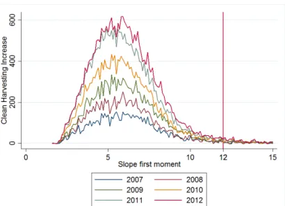
Figure A3: Mechanical Harvesting vs Slope

This figure presents mechanical harvesting in year t divided by mechanical harvesting in 2006 per value of slope first moment. To do this we round slope first moment to the first decimal place, so we have more observations at one slope first moment point. We drop slope first moment values greater than 15% because of very few observations.

Figure A4: Planted Area Expansion vs Slope

This figure presents presents planted area in year t divided by mechanical harvesting in 2003 per value of slope first moment. To do this we round slope first moment to the first decimal place, so we have more observations at one slope first moment value. We drop slope first moment values greater than 15% because of very few observations.

(32)

Table A.1: Pre-trend – Manufacturing sector

Pre-trend for manufacturing sector ∆2000-1991

(1) (2) (3) (4) (5) (6)

Panel A. Employment share

Clean Adoption Index -.038 -.0637* -.0753** -.0375 -.0409 -.0777**

(.0316) (.0324) (.0348) (.0314) (.0358) (.0345)

Panel B. Unskilled employment share

Clean Adoption Index -.0475 -.0758** -.089** -.0478 -.0553 -.0961**

(.0342) (.0359) (.0366) (.0341) (.0381) (.0374)

Panel C. Skilled-unskilled workers ratio

Clean Adoption Index .3018** .2323* .3476** .2877** .3005* .257

(.1403) (.1408) (.15) (.1422) (.1623) (.1613) 1st Stage (KP F-stat.) 19.18 20.75 19.17 18.84 15.21 16.37 Education Y Y Population density Y Y Distance to roads Y Y Soil suitability Y Y

Notes: This table displays the estimates of adoption of mechanical harvest on multiple variables (as indicated in the Panels) as captured by β in equation (2). All regressions are controlled for the share of rural population in 1991, the log of labor force in 2000, and the the log of sugarcane planted area in 2003. Education controls include the share of illiterates and of skilled workers in 1991. Population density control is measured in 1991. Distance to roads are in log. Soil suitability for sugarcane from GAEZ/FAO. The unit of observation is ´Area M´ınima Compar´avel (AMC) (N = 351). Robust standard errors reported in parentheses. *** p< .01, ** p< .05, * p< .1.