Disturbing the fiscal theory of the price level: can it fit the EU-15?

DISTURBING THE FISCAL THEORY OF THE PRICE

LEVEL: CAN IT FIT THE EU-15?

António Afonso (**)

Department of Economics, Instituto Superior de Economia e Gestão, Universidade Técnica de Lisboa,

R. Miguel Lúpi, 20, 1249-078 Lisbon, Portugal This version: January 2002

Abstract

With the fiscal theory of the price level (FTPL), Leeper-Sims-Woodford (LSW) argued that the government budget constraint plays a key role in determining the price level. Indeed, there could even be a dispute vis-à-vis the role of monetary policy in the formation of the price level. Apart from several theoretical criticisms, also addressed in the discussion given in this paper, the attempts to validate empirically the novel theory are, so far, rather sparse. Additionally, one of the purposes of this paper is to tentatively assess the possible empirical evidence, concerning the FTPL, for the EU-15 countries.

Keywords: Fiscal theory of the price level; fiscal policy; EU-15; panel data models JEL classification: C23; E31; H63

(*) _{This paper was in some way inspired by the research conducted for the author’s Ph.D. thesis.}

The author acknowledges comments from Jorge Santos. The usual disclaimer applies.

Contents

1 - Introduction ...…... 3

2 - The fiscal theory of the price level set-up……… 4

2.1 - Ricardian versus non-Ricardian regimes……… 4

2.2 - The critics from the fiscal theory to the monetarist explanation…………. 8

2.3 - The price level fiscal theory approach………. 12

3 - A critical discussion of the fiscal theory………... 18

4 - Validation of the fiscal theory of the price level………... 25

4.1 - Budget deficits and public debt………... 27

4.2 - Some evidence for the EU-15………. 29

5 - Conclusion……… 37

Annex ……… 39

1 - Introduction

The fiscal theory of price level (FTPL), developed by Leeper (1991), Sims (1994) and Woodford (1994, 1995), relates to an already well known discussion in the literature, about whether fiscal policy plays a role, as important as monetary policy, in determining

the price level.1 There is also a connection to the controversy concerning the use of rules

to determine the nominal interest rate, that, as mentioned by Sargent and Wallace (1975), leave the price level undetermined, therefore LSW argue that the government

budget constraint is crucial for the price level determination.2

The main point behind the FTPL is indeed the idea that the price level is determined through the inter-temporal government budget constraint. That is, the price level adjusts in order to assure that the value of nominal government debt, divided by the price level, equals the real present value of future budget surpluses. In other words, the price level equals the ratio of nominal government liabilities to the present value of future budget surpluses in real terms.

The literature on the FTPL has increased substantially, rendering difficult an exercise of keeping up with all the incoming references on the topic. Nevertheless, one can mention namely some papers by Woodford (1996, 1998a, 1998b, 2001), Cochrane (1999, 2000, 2001) and Sims (1999). The use of the FTPL in an international framework - two countries, exchange rate determination, and monetary union - is discussed by Woodford (1996), Sims (1997, 1999), Dupor (2000), Bergin (2000), Canzoneri, Cumby and Diba (2001), Andrés, Ballabriga and Vallés (2000) and Daniel (2001). Loyo (2000) addresses the inflationary episodes in Brazil using the FTPL while Sims (2001) makes a similar attempt to assess the consequences of dollarization in Mexico. Also in the context of the

1

The expressions "fiscal theory of price determination" (see Canzoneri and Diba (1999)) or "fiscal theory of money" (see Marimon (1999)) appear also in the literature. Coleman (1995) favours the use of the terminology “fiscal regime of price level determination.”

2

According to Buiter (1999) the inspiring contribution is credited to Begg and Haque (1984), even if this is a less mentioned paper in the literature. As a matter of fact, and as Auernheimer and Contreras (1991) mention, "An understandable reason why the Begg and Haque results are not cited in any of the current literature is that they were published in a journal of limited audience. In fact, we became aware of the existence of the paper by merely coincidental conversation with one of the authors."

FTPL, Corsetti and Mackowiak (2000) discuss and relate the occurrence of currency devaluations to the existence of fiscal unbalances.

Critical discussions of the theory and of its assumptions are offered namely by McCallum (1999a, 1999b, 2001), Buiter (1998, 1999, 2001) and Bassetto (2001), while explanations of the theory can be found in Kocherlakota and Phelan (1999), Christiano and Fitzgerald (2000) and Carlstrom and Fuerst (2000). Concerning the empirical testing of the theory, the literature is rather small, but one can mention the papers of Canzoneri, Cumby and Diba (1997, 2000), Cochrane (1999) and Woodford (1999), Mélitz (2000) and Creel and Sterdyniak (2000).

This paper adds to the literature, by offering a critical discussion of the theory and by trying to assess the empirical evidence concerning the feasibility of the FTPL, for the EU-15 countries, with panel data estimations. The remaining of the paper is as follows. Section two presents the FTPL, section three gives a critical overview of FTPL, section four tentatively evaluates the empirical evidence for the EU-15, and section five is the conclusion.

2 – The fiscal theory of the price level set-up

Underlying the work developed by LSW, is the idea that for some combinations of fiscal and monetary policy, the price level is determined by the ratio between government nominal liabilities and the real present value of future government assets (budget surpluses). This is an important issue since central banks seem to be now less enthusiastic in using monetary rules for their monetary policy decisions. The implementation of such rules is usually regarded as an attempt to capture the visible historical relationship between money and prices.

2.1 – Ricardian versus non-Ricardian regimes

The set-up for the FTPL may be understood on the basis of the categorization of two types of fiscal regimes, the way is done for instance by Woodford (1995): Ricardian versus non-Ricardian regimes. Actually, this classification had already been done by Aiyagari and Gertler (1985) who maintained that in a non-Ricardian regime the

Treasury does not commit itself to match completely, in the future, new public debt with future taxes, since some part of the new debt is to be financed through money, the opposite of what would happen in a Ricardian regime. Benhabib, Schmitt-Grohé and Uribe (2001) assume also this kind of classification.

In a Ricardian regime, primary budget balances respond to the level of government debt in order to ensure budget solvency. In this case, money and price level may be determined by the supply and demand of money and one may consider that there is an active monetary policy/strategy. In other words, one is assuming that the effects of government deficits on prices, interest rates and income are irrelevant, in line with the Ricardian equivalence assumptions.

Indeed, in a non-Ricardian regime, the government could determine primary budget balances, regardless of the level o public debt. In this case, money and prices would adjust to the level of public debt in order to ensure the fulfilment of the government budget constraint. This is the main characteristic of the FTPL.

Canzoneri and Diba (1996) use another terminology, already adopted by Sargent and Wallace (1981). While the Ricardian regime is tagged as a "regime of monetary predominance", since money demand and supply determine in this case the price level, the non-Ricardian regime is labelled "a regime of fiscal predominance," as prices are now endogenously determined from the government budget constraint.

Buiter (1999) offers several criticisms against the FTPL, and also deals with this issue as an opposition between two fiscal rules for the government behaviour: the government might follow a “Ricardian fiscal rule” or a “non-Ricardian fiscal rule.” Implicit in the use of the Ricardian rule is the hypothesis that the inter-temporal government budget constraint will be fulfilled for all the sequences of endogenous variables. In the case of a non-Ricardian rule there is implicitly the assumption that the inter-temporal government budget constraint is only met for equilibrium values of the endogenous variables. The several expressions used in the literature, to label the two regimes of fiscal and monetary policy, are summarized in Table 1.

Table 1 – Fiscal versus monetary regimes: some terminology in the FTPL framework

Reference Terminology

Leeper (1991) Passive strategy from the Treasury;

Active strategy from the Central Bank

versus Active strategy from the

Treasury;

Passive strategy from the Central Bank

Aiyagari and Gertler (1985), Woodford (1995)

Ricardian regime versus Non-Ricardian regime

Canzoneri and Diba (1996)

Monetary regime dominance

versus Fiscal regime dominance

Buiter (1999) Ricardian fiscal rule versus Non-Ricardian fiscal rule

Going back to the “game of chicken” mentioned by Sargent (1986), about the “dispute” between the Treasury and the Central Bank, the quantitative money equation and the government budget constraint equation may reflect the effects, upon the price level, of the preponderance of either a Ricardian or a non-Ricardian regime.

Therefore, in a regime where the monetary policy is independent (active), as in a Ricardian regime, the monetary authority determines the money stock and the price level through a money demand equation, based on the quantitative theory of money. The government is in this case required to attain primary budget surpluses, in order that its budget constraint is consistent with the price level resulting from the money demand equation. There is then, according to Leeper’s (1991) terminology, a passive strategy

from the Treasury and an active behaviour from the Central Bank.3

In a non-Ricardian regime, where the Treasury decides autonomously the values of the budget deficit and of the public debt, the price level may be determined independently from the monetary authority. In this case, the Central Bank assumes a passive attitude, money supply is endogenous, and the price level is determined by the government

budget constraint.4 The FTPL could then be appropriate if the government did not

choose a passive fiscal policy, that is, when the budget surpluses are not adjusted endogenously in order that the budget constraint satisfies the price level implicit in the money demand function.

3

Dotsey (1996) distinguishes between independent and dependent monetary policy.

4

For instance Cochrane (1998) argues that the government budget constraint "will determine the price level no matter what the rest of the economy looks like (...)."

This framework has some reminiscence of the popular unpleasant monetarist arithmetic case of Sargent and Wallace (1981), which is basically the result of a situation where the monetary authority reacts passively to an active fiscal policy put forward by the government. In fact, in the set-up of Sargent and Wallace, there is first an atempt by the authorities to implement simultaneously a regime of fiscal dominance and a regime of monetary dominance. However, even in the context of the unpleasant monetarist arithmetic, in the end, inflation is still viewed as a monetary result. With the FTPL hypothesis, fiscal policy may determine the price level even if there are no changes in the money stock.

For instance, Carlstrom and Fuerst (2000) classify the approach of Sargent and Wallace (1981) as the “weak-form” of the FTPL, since even if the exogenous fiscal policy infuences prices, this is done through the money suply, which is endogenous. In the more recent LSW explanation, fiscal policy determines the price level independently of the money supply, leading Carlstrom and Fuerst to label this approach as the “strong-form” of the FTPL.

Also, Gordon and Leeper (2000) assume three versions of the FTPL; the first one explained along the lines of the work of Sargent and Wallace (1981) who, like Aiyagari and Gertler (1985), argue that inflation remains essentially a monetary matter, even though there are constraints imposed by fiscal policy. The second version would be the one defended by the work of Leeper (1991), Sims (1994) and Woodford (1994, 1995) that call attention upon the fact that money, public debt, and fiscal policy, jointly determine the price level. Still a third version of the FTPL seems to be discussed by Woodford (1995, 1998a) and Sims (1997), who try to establish that the equilibrium price level may be determined only by fiscal variables, in other words, the price level would be independent from the path of money stock. Additionally, Cochrane (1999) suggests a more controversial version of the FTPL, where the existence o money is superfluous, and where monetary policy would be unimportant to historically explain

inflation.5

5

Bohn (1999) and Woodford (1998) give some critical comments on this extreme version of the FTPL.

2.2 - The critics from the fiscal theory to the monetarist explanation

The FTPL argues against the assumption, suggested namely by Friedman, that inflation is purely a monetary problem. For instance, Woodford (1995) questions the idea, keen to the quantitative theory of money, that the Central Bank should control the money stock in order to attain price level objectives. The proponents of the FTPL maintain that even if there is no change in money stock, fiscal policy may independently affect the price level and the inflation rate. This situation may arise either from the possibility that the Central Bank does not control the money supply, or due to the hypothesis that inflation may not, in fact, be a monetary issue.

When there is an increase in the price level, there will be as a consequence the decline of the real value of the government liabilities, understood here as the pooled liabilities of both the Treasury and the Central Bank. These liabilities comprise therefore the stock of government debt, in possession of the public, and the stock of monetary base. As a result of the price level rise, there is a negative wealth effect through the reduction of the real value of the individuals applications, for instance in government debt. Hence, there may occur a decrease of aggregate demand, with prices adjusting aggregate demand and supply in the short run. For instance, with a fixed money supply, the increase of the budget deficit may be accompanied by the rise of prices, allowing the decrease of the real value of public debt, in order to guarantee the fulfilment of the government budget constraint.

Following the above reasoning, one may recall the weak correlation between money and prices since the start of the 80s, in most of the industrialized countries, with the progressive abandon of monetary aggregates as an intermediate objective of monetary

policy.6 This is for example (see Figure 1) the case of the US where there seems

6

"Throughout the English-speaking world, at least, central bankers have abandoned the notion that any of the conventional monetary aggregates constitute a suitable intermediate target for monetary policy. This has resulted from the discovery that these aggregates no longer appear to have any very reliable relationship, at least in the short run, with the variables, such as inflation and real activity, about which policymakers actually care" (see Woodford (1998b)). The same point is made by Romer (2000): “(…) most central banks, including the U.S. Federal Reserve, now play little attention to monetary aggregates in conducting policy.”

obvious the lack of a positive relationship between inflation and monetary base since

the begining of the 80s.7

Figure 1 – Annual change of Monetary Base and inflation in the US

0 2 4 6 8 10 12 1960 1963 1966 1969 1972 1975 1978 1981 1984 1987 1990 1993 1996 1999 Inflation Monetary Base

Source: European Economy 72, 2001. European Commission (inflation);

Federal Reserve Statistics Release, Historical Data, H.3 (Monetary Base).

Of course, and as stressed by Cochrane (1999, 2000), the specification of a money demand equation, through which prices are supposed to be monitored according to the quantitative theory, implies that fiscal policy will afterwards adjust endogenously to the resulting price level.

Lets now consider the traditional relation of the quantitative theory of money, between money and income,

t t t tv Py

M = (1)

where M is nominal money, P is the price level, y is real income and v stands for the

income-velocity of money.8 Assuming, for instance, that the income-velocity of money

depends on the nominal interest rate, vt=v(it),9

7

Dwyer and Hafer (1999) review some of the latest evidence concerning the relationship between monetary growth and inflation.

8

Naturally, the classic reference for the identity of the quantitative theory of money is Fisher (1911, p. 24-32). The relationship between real money and income may also be presented as M/P = ky where the proportionality factor k (k=1/v) is the notation used by Pigou (1917).

t t b t t i Py M ( ) = (2) b>0,

using logarithms and the real effective interest rate, r, with perfect prediction, it is possible to write

[

]

For simplification sake, it is possible to assume that income, the money supply and the real interest rate are constant,

[

]

t y b r P P

P

M ln ln ln ln ln

ln = + − + ₊₁− (4)

and then we have the following difference equation for the price level

[

]

Hence, according to the initial price level, there is an infinite number of possible trajectories for the previous equation. The usual solution is to assume/choose the initial price level obtained from

r y M

P ln( / ) ln

ln ₀ = − , (6)

in order to ensure that the price equation does not lead to an explosive trajectory. One of the critics put forward by Woodford (1994, 1995), is that this choice for the initial price level has no support on economic theory and it is not derived, for instance, from some money demand function optimisation.

9

One of the results of the monetarist theory is that the use of rules to determine the interest rate ends up in an indeterminacy for the price level, and the Central Bank may eventually loose control of the inflation rate. In fact, in this case, money supply is hopeless to uniquely determine the price level. The classic text is Sargent and Wallace (1975), where it is shown that price level is indeterminate when an interest rate rule is used and when prices are flexible. A clear exposition of this point is given namely by Blanchard and Fischer (1989, p. 577-582), but the issue can be tracked back to Wicksell

(1965 [1898], 1907).10

However, the point made by LSW is that if consumers are non-Ricardian, and in the context of a non-Ricardian fiscal regime, the wealth effects should show up through nominal government debt, with the government budget constraint being then used to determine a unique price level. Therefore, the proponents of the FTPL defend that the price level is indeed determined by the government budget constraint,

∑

where Bt stands for the government nominal liabilities in period t, including the stock of

public debt (for simplicity one year securities) and monetary base; st is the primary

budget government surplus in period t, including seigniorage revenues, in real terms; r is the real interest rate, assumed constant, and considering also the usual transversality condition 0 ) 1 ( lim 1 = + ∞ → + s+ s t r B s . (8)

A possible analogy for the government budget constraint may be to think of the stock of public debt as a government bond, with periodic coupon payments, and where the primary budget surpluses are the coupons. In this case, the changes in the price level can be considered as resulting from the variations in the market value of this special government bond.

10

This topic attracts attention from economists on a regular basis. See for instance Patinkin (1965) and Bénassy (2000).

However, it is relevant to bear in mind that fiscal and monetary policy, directly or indirectly, both end up being responsible for the fulfilment of the government budget constraint. Equation (7) will be successfully met if the government adopts a non-Ricardian fiscal policy, using Woodford’s terminology. Therefore, after the government having arbitrarly chosen a sequence of fiscal balances, by choosing the level of public expenditures, the price level will adjust endogenously to ensure compliance with the budget constraint. In other words, if equation (7) is to be met for any value of price level, than fiscal policy must adjust passively (Leeper [1991]), in line with a Ricardian regime (Woodford [1995]).

2.3 - The price level fiscal theory approach

For the presentation of the FTPL framework, lets assume a model of numerous and infinitely lived households that maximize an utility function with money as an argument. This type of money-in-the-utility-function (MIUF) model is inspired in Sidrauski (1967) and Brock (1975) and the utility function of the consumers, supposed to be additive, may be written as

η σ _η σ − − _{+ −} − − − = 1 2 1 1 1 1 ) 1 ( ) 1 ( ) , (ct mt Act A mt U , (9) σ>0; η>0;

where ct is consumption in real terms in period t, mt = Mt/Pt, and M is the nominal stock

of money.11

The budget constraint for the households, in nominal terms, may be written as

t t t t t t t t t B i B M M c P tx y P − + + − + = − + + 1 ) ( 1 1 (10) 11

The utility function used here (inspired in McCallum (1999a)) is basically a parametric version of the general formulations used by Leeper (1991) and Woodford (1995).

where y is the output, assumed constant, txt are the lump-sum taxes paid in t, Bt stands

for one period government debt securities, outstanding in period t, and i is the nominal interest rate.

The previous constraint may also be presented in real terms as

t t t t t t t t t t t t t t t P B i P P P B P M P P P M c tx y − + + − + = − + + + + + + 1 1 1 1 1 1 1 1 , (11)

defining bt = Bt/Pt and multiplying both members of the last equation by (Pt/Pt+1), we

have also t t t t t t t t t t t t t t t b P P b i m P P m c P P P P tx y 1 1 1 1 1 1 1 1 ) ( + + + + + + − + + − + = − . (12)

The utility optimization problem of the households is then given by,

     − + + − + = − + − = + + + + + + − − − − t t t t t t t t t t t t t t t t t b P P b i m P P m c P P P P s m A c A m Max 1 1 1 1 1 1 t 1 2 1 1 1 1 t 1 1 ) tx -(y a . ) 1 ( ) 1 ( ) , U(c σ σ η η , (13)

with the following first order condition for the optimum solution,12

) , ( 1 1 ) , ( 1 _{1 1} 1 + + + + + + = c t t t t t t t c U c m r i P P m c U , (14)

the usual Euler equation, now depicting addionally the use o money in the households utility function.

The consolidated government budget constraint (including the Central Bank) is as follows,

12

t t t t t t t t B i B M M tx g P − + + − = − + + 1 ) ( 1 1 , (15)

with the budget deficit financed, either by the issuance of money, either by the issuance

of public debt. Bt+1 are government bonds issued in period t, at price 1/(1+it), to be

reimbursed in period t+1 for one monetary unit, and gt and txt are respectively the

government expenditure and taxes in real terms, in period t. The budget constraints of the households and of the government imply the following equilibrium condition for the goods and services market in the economy, after adding (10) and (15),

t

t g

c

y = + . (16)

In real terms the government budget constraint can also be presented as

t t t t t t t t t t P B P i B P M M tx g − + + − = − + + 1 1 1 1 (17) t t t t t t t t t t t t t t t P B i P P P B P M P P P M tx g − + + − = − + + + + + + 1 1 1 1 1 1 1 1 (18)

and, using once more the definitions bt = Bt/Pt and mt = Mt/Pt, it is possible to write the

government budget constraint as

t t t t t t t t t t t b i P P b m P P m tx g − + + − = − + + + + 1 1 1 1 1 1 . (19)

By definition, the real interest rate is given by the Fisher relation,

) 1 )( 1 ( 1 e₁ t t t r i = + + ₊ + π (20)

and supposing that the price level is correctly predicted for t+1, that is, assuming

perfect forecast for the expected inflation rate, π (with _{t 1}e₊ P_te₊₁ =P_t+1),

t t t t e t P P P − = = + + +1 π 1 1 π , (21)

this allows us to write

      ₊ − + = + + t t t t t P P P r i (1 ) 1 1 1 (22) t t t t P P r i 1 ) 1 ( 1+ = + + . (23)

Bringing to mind the situation mentioned above, where the monetary base growth rate is constant, and substituting the inverse of (23) in (19), results in

t t t t t t t t t b g tx P P r P P b = + − + ₊ + + 1 1 1 1 1 (24) ) )( 1 ( ) 1 ( 1 t t t t t t r b r g tx b₊ = + + + − (25)

and, assuming also the hypothesis of a constant real interest rate, we finally get

) )( 1 ( ) 1 ( 1 t t t t r b r g tx b₊ = + + + − . (26)

Additionally, and for simplicity, if the budget deficit is stable, (g_t −tx_t)=(g−tx), we

have also ) )( 1 ( ) 1 ( 1 r b r g tx bt+ = + t + + − , (27)

and, from the the last expression, it becomes clear that bt = Bt/Pt will follow an

explosive trajectory since (1+r)>0. Figure 2 illustrates the government fiscal constraint and the evolution of the stock of public debt, based on equation (27), which can be written succinctly as ) )( 1 ( 1 r b s b_t+ = + _t − (28)

where the primary budget surplus, s, is given by s = tx-g.

Figure 2 – Government debt path (real terms)

Starting from an initial value for bt in the horizontal axis, going perpendicularly up to

the line (in full) of the budget constraint and then horizontally to the 45 degrees line, and then again vertically to the budget constraint line, it is easy to witness the explosive evolution of government debt.

If there is an initial value for the stock of real government debt, bo, below b*, b diverges

restriction for the stock of real public debt. For b > b*, the stock of real public debt diverges also, and the value follows an explosive path. Notice that the growth rate of government debt, from equation (28), is given by the following difference equation

) 1 )( 1 ( 1 t t t b s r b b − + = + _{, (29)}

that eventually converges to (1+r) while b increases. However, in this case, the government is conducting Ponzi games, and it would no be possible to satisfy a transversality condition such as the one given by equation (8).

An explosive situation for the stock of real government debt will be avoided if the initial

value for b , b0=b*, is r tx g r b0 =−(1+ )( − )/ , (30)

in order to ensure that b remains constant at that same value.13 As a matter of fact, with

that initial value for b one gets

) ( 1 g tx r r P B t t _ −      + = . (31)

Therefore, according to the FTPL, P0 is determined by the previous expressions and is

given by

[

]

To prevent the explosive outcome underlying bt+1 =(1+r)bt +(1+r)(g−tx), it is necessary that the starting point fulfils the following condition: b₀ =(1+r)b₀ +(1+r)(g−tx), simplifying, it is required that b₀ =−(1+r)(g−tx)/r. In this case it is also easy to verify that we will have

in other words, the price level is endogenously determined from the ratio between the

initial public debt level and the government balance.14

3 - A critical discussion of the fiscal theory

As already mentioned, the FTPL sees the price level as resulting from fiscal policy decisions, in contrast with the monetarist explanation of the quantitative theory of money. In a Ricardian regime, of monetary dominance, the nominal value of government debt (or in a broader sense the government liabilities) results from the accumulation of budget deficits. If the price level is determined by the quantitative theory of money, the real value for the stock of public debt comes out endgenously and the present value of future budget surpluses must adjust in order to meet the government budget constraint.

In the case of a non-Ricardian regime, of fiscal dominance, the real value of the stock of public debt is determined by the present value of future budget surpluses, and the price level that must adjust to gurantee the fulfilment of the budget government constraint. What we have here is then two different interpretations on how the adjustment of the several variables takes place in the framework of the government budget constraint. For instance, Cochrane (2001) maintains that Ricardian regimes are backward-looking, in the sense that the real values of the stock of public debt is determined by the price level and by past budget deficits, while a non-Ricardian regime is forward-looking, since it is now the real value of the stock of public debt, set accordingly with the present value of future budget surpluses, that will determine the price level.

Price level indetermination is directly related to the fact that the Central Bank may use monetary policy to determine the nominal interest rate. In this case, with the nominal interest rate set exogenously by the monetary authority, the equation of the quantitative theory of money, equation (1), and the equation for the price level change, equation (23), are used to determine the money stock and the price level (assuming a constant real interest rate). However, equation (23) only determines the inflation rate and not the

price level, that is, Pt is undetermined. In this situation, the relation of the quantitative

14

Sims (1997, p. 8) labels this approach as “"quantity theory of [public] debt" determination of the price level.”

theory of money determines the money stock in a passive way, which adjusts to the desired interest rate level, but it is unable to determine the price level. This undetermination may be solved through the government budget constraint, equation (7), that now determines the price level, the solution forwarded by the proponents of the

FTPL.15

As an alternative, if the monetary authority decides to determine the money supply, then, in a Ricardian regime, of monetary dominance, equations (1) and (23) may determine with no further problems the price level and the nominal interest rate. In this case, the government budget constraint is always satisfied and will not be used to determine the price level. Also, if the Central Bank tries to set an objective for the money supply, when the government is carrying out an active fiscal policy, that is, a non-Ricardian regime, the price level may be overdetermined. Table 2 summarises these results.

Table 2 – Fiscal determination of price level and monetary policy

The monetary authority tries to set: the nominal interest rate a monetary aggregate Ricardian regime,

monetary dominance

In this case the price level is undetermined (*)

The price level is determined, using the quantitative relation of money

Non-Ricardian regime, fiscal dominance

The price level may be determined by the government budget constraint (**)

The price level is overdetermined

(*) The case mentioned by Sargent and Wallace (1975). (**) Leeper (1991), Sims (1994) and Woodford (1994,1995).

Buiter (1998, 1999, 2001), one of the critics of the FTPL, argues that the theory proposed by the work of LSW is what he calls “the pure fiscal theory of the initial price level” (Buiter [1998, pp. 25]). In fact, Buiter (1998) mentions that the initial price level is determined by equation (31) and is proportional to the stock of non-monetary liabilities (public debt), and this could be understood strictly as what the author mentions as the “quantity theory of nominal bonds.” However, and taking into account the initial price level, in the following periods prices will be determined by equation

15

Schmitt-Grohé and Uribe (2000) and Carlstrom and Fuerst (2001) discuss the issue o nominal and real indeterminacy in MIUF models.

(23). Besides, the nominal stock of money has an effect on the nominal interest rate, that is, for a given level of public debt and prices, an increase of the money stock implies a decrease of the nominal interest rate and, with a constant real interest rate, there should be a decrease of the future nominal value of government debt. The decline of public debt will then lower the price level, and so Buiter maintains that money still influences prices.

Buiter stresses also the fact that it does not seem reasonable that the government uses the budget constraint (7) to determine the primary balance and the issuance of public debt, without taking into account a given price level. Also, the models presented by the proponents of the FTPL, give the impression that they are determining a level of public debt default and not so much the price level. If the responsibles of economic policy were to adopt the ideas of the FTPL, there would end up to appear either situations of default on public debt reimbursements or situations of hyperinflation.

Cochrane (2000) answers back to Buiter’s criticisms by saying that Buiter is taking for granted a Walrasian formation of prices in the market, were no transaction occurs until the adequate price level is met, in order to validate the budget constraint. However, and since it is not possible to know beforehand which is that price level, nothing will prevent the government of deciding the indebtedness level and the primary balance that it wishes to assume. If the government did behave like Buiter seems to be suggesting, disregarding market restrictions, the level of public debt might rise without limit when, in fact, the equilibrium price level is adjusted to prevent that such boundless increase of government debt might occur.

Cushing (1999) argues that in a non-Ricardian regime, chacterized by an active fiscal policy, the fiscal determination of the price level requires some rather implausible assumptions. For instance, in order to determine the price level through the intertemporal budget constraint, it is necessary for the consumers to believe that the government will honour its debts, even when the stock of public debt rises to very high levels. If there is a significant risk that those debts are not paid, the government may have to change the way it conducts fiscal policy, to ensure that its intertemporal budget constraint is not violated, since the alternative, a price level increase, would reduce the real value of debt to be reimbursed to the public, that might not buy, in the future, new

government debt in the market. In these circumstances, the price level would not be determined by the government budget constraint, instead, the price level ends up being a restriction to which that constraint must obey. Cushing (1999), as well as McCallum (1999a), criticise therefore the FTPL supposition of the transversality condition and the hypothesis that the stock of public debt is on a convergence path. In a non-Ricardian regime, neither the government nor the Central Bank are committed to ensure that convergence process, however, the public is supposed to believe that the government will not default in the future on its liabilities.

The essence of the FTPL, in its criticism of the quantitative theory of money, does not seem to be to figure out if the quantitative equation of money links or not the price level with the stock of money, but really to discuss if the stock of money and the price level may be determined by fiscal policy. However, to distinguish between if the supply of money and the interest rate are determined by fiscal policy or if the money supply and interest rate are determined exogenously, it is not an easy point to assess only under theoretical grounds.

In empirical terms, there appears to be some evidence that could be read as being for and against the FTPL. For instance, the well known cases of hyperinflation in Europe in

the beginning of the 20th century, discussed by Cagan (1956) and by Sargent (1982),

seem to indicate that the inflationary periods of Germany, Austria, Hungary and Poland were only surpassed after the problems in terms of fiscal deficits had been delt with. When studying the monetary characteristics of hyperinflations in Austria, Hungary, Poland and Russia in the 20s and in Greece, Hungary and Russia in the 40s, Cagan (1956) used models for money demand based on the strong relation existing between

money and inflation.16 In Cagan’s (1956, p. 85) words, it is possible to understand the

idea that the government financing needs were one of the causes of hyperinflation:

“(…) taxes yielded some revenue, of course, though presumably an amount insufficient for desired total expenditures. As the rate of price increase rose, however, the real value of whatever funds were raised by other taxes

16

A posteriori, the econometric problems of those models were pointed out namely by McCallum (1989).

undoubtedly diminished, and during the later stages of hyperinflation these funds must have become nearly worthless owing to delays in collecting them.”

Loyo (2000) explains the hyperinflation of Brazil in 1975-1985 as a result a of a vicious circle between the nominal growth of government debt and the corresponding rollover of existing debt. Also, Woodford (1999, pp. 393) maintains that fiscal policy in the US might have been non-Ricardian before 1951: “That period would represent a historical example of the kind of interest-rate pegging regime for which the theory was

developed.”17

In the first half of the 70s, the idea of a regime of fiscal dominance, Ricardian in Woodford’s terminology, may be relevant, since there was a decline of fiscal balances and an increase of inflation, namely in Italy and in the UK, see Figure 3 and Figure 4, and also for instance in the US. Also, and as mentioned by Sargent (1987), the fact that the government budget constraint is pratically absent from macroeconomic models in the 60s and 70s, may be an indication that the budget constraint was then seen more like an equilibrium condition and less as constraint.

Figure 3 – General government balance and inflation: Italy

Italy -14 -12 -10 -8 -6 -4 -2 0 1970 1972 1974 1976 197 8 19 8 0 19 8 2 19 8 4 19 8 6 19 88 1990 1992 1994 1996 199 8 2000 -3 2 7 12 17 22

Gov. bal. Inflation

Source: European Economy 72, 2001. European Commission.

17

It was in March 1951 that was made the accord between the US Treasury and the Central Bank in order to give the Central Bank more autonomy to change interest rates, Hetzel and Leach (2001) give a reading of the implications of that agreement.

Figure 4 – General government balance and inflation: UK UK -8 -6 -4 -2 0 2 4 6 1970 1972 1974 1976 197 8 19 8 0 19 8 2 19 8 4 19 8 6 19 88 1990 1992 1994 1996 199 8 2000 0 5 10 15 20 25

Gov. bal. Inflation

Source: European Economy 72, 2001. European Commission.

In the beginning of the 80s there was an increase of budget deficits in several western economies. According to the assumptions of the FTPL, there should have been a price level rise in order to reduce the government liabilities in real terms. For instance, in Italy, see Figure 3, there was a decline of inflation throughout the 80s, what seems to disagree with the FTPL.

This sort of interpretations is rejected by Cochrane (1999) who tries to reconcile these data with the FTPL, arguing that real primary deficits determined inflation, since after the middle of the 80s there were improved expectations concerning future budget surpluses. Hence, when there are changes in the expectations about the level of future budget balances, the present value of fiscal balances is also adjusted, and this must be reflected on the change of the government liabilities, through price level changes. Therefore, with this reasoning, it is interesting to mention that in the 90s, at the same time that the US budget deficit declined, becoming even a surplus after 1998, it was possible to see a sustained decrease of the inflation rate.

Also, it is also relevant to distinguish between the money measure included in the equation of the quantitative theory of money and the monetary liability used in the government budget constraint. Indeed, in the equation of the quantitative theory of money, for instance equation (1), money is seen as a broader monetary aggregate (M1,

M2 or even M3) than the monetary base used to to quantify the seigniorage revenues in the government budget constraint, equation (7).

Assume, for example, that the monetary authority reduces the money supply. If there is a Ricardian regime, of monetary dominance, the decrease of money supply should result in a drop of the price level. Notice also that this price level decline will bring about an increase of the real value of the outstanding stock of public debt, and, in the future, the government will have either to raise taxes or to cut public expenditures, in order to meet the budget constraint.

If there is a non-Ricardian regime, of fiscal dominance, a decrease in the money supply dose not affect the price level since this variable is now determined through equation (31). However, the equilibrium price level should now be smaller than the one that was in place previously to the money supply cut, in other words, there might be too much inflation. This situation would be possible if the government did not obey, for some time, its budget constraint. The budget constraint would then only be fulfilled for a long-run equilibrium situation, which seems to be a rather strong assumption. As a matter of fact, the government budget constraint is, by construction, an identity that should hold at any point in time. Eventually, if for instance the reduction of money supply was associated to a tax raise, then the money supply decrease would end up in a price level fall, either through money demand, based on the quantitative theory of money, where prices decrease on a one to one basis with the change of money stock, either through equation (31).

The main feature of the government budget constraint, the fact that public debt can not go beyond the value of present and future budget surpluses, should be met, either in equilibrium or not. This characteristic of the government constraint does not seem to be adopted by the proponents of the FTPL, who assume that the budget constraint must be fulfilled only in equilibrium, a hypothesis that is hard to sustain. See for example the comments forwarded by Woodford (1998a, p. 17-18)):

“Note that our argument does not involve any denial that the value of the public debt must actually equal the present value of future government budget surpluses, in equilibrium. What we deny is that condition (1.14) [the initial value

of public debt is equal to the present value of current and future budget surpluses plus seigniorage] is a constraint upon government fiscal policy, that must be expected to hold regardless of the evolution of goods prices and asset prices. Instead of a "government budget constraint", the condition is properly viewed as an equilibrium condition, that follows from the joint requirements of

private sector optimisation and market clearing.”18

Still another point assumed by the FTPL is also open to criticism: the assumption that the government allways intends to rollover a fraction of the outstanding stock of public debt. However, if the successive budget surpluses allow to significantly reduce the stock of public debt, the hypothesis that the price level is determined by the intertemporal government budget constraint, equation (7), implies that the price level would approach zero. Notice that some of the EU-15 countries (for instance Ireland, Denmark, Finland, United Kingdom) countries and the US, had in the last years consecutive budget surpluses, resulting in the reduction of the stock of public debt, without significant changes in the inflation rate.

Additionally, a contribution for an increase of inflation might be the occurrence of defaults on interest rate payments and reimbursements of public debt. These situations may then reduce the present value of future budget surpluses and the price level would then have to rise to ensure once more the fulfilment of the intertemporal government

budget constraint.19

4 - Validation of the fiscal theory of the price level

Regarding the empirical validation of the FTPL, Cochrane (1999) doubts of the interest of that validation, that is, of the interest in assessing empirically the suitability of a non-Ricardian regime, since the causal relations between the several variables can never be rejected/accepted without making use of additional assumptions, frequently stemming from the hypothesis itself made about the fiscal regime that is tested. It seems however

18

Still on the budget constraint, it does not seem clear the idea forwarded by Cochrane (2000) that sees the constraint not as a restriction but like a “government valuation equation.”

19

that this is also true with the identity of the quantitative theory of money and the resulting money demand functions.

For example, Woodford (1995) also contends that it does no make much sense to test in empirical terms the FTPL. The line of reasoning provided is based on the idea that all monetary regimes, monetary rules ourmoney demand specifications leave the price level undetermined, and consequently the price level can only be determined by the fiscal

policy.20

The solution of trying to validate the FTPL through the inspection of budget deficits and government debt, a possible empirical approach, is not easy since in a non-Ricardian regime there is solely the guarantee that the government budget constraint is obeyed in equilibrium (see Cochrane [1999] and Woodford [1998a]). This conviction is also criticised by Buiter (1999) who says that “…the government's intertemporal budget constraint is a constraint on the government's instruments that must be satisfied for all admissible values of the economy-wide endogenous variables.”

The government budget constraint, equation (7), and the usual transversality condition, equation (8), may give a suggestion on how to assess the adjustment process of the main fiscal variables. A possible method would be to try to understand wether is the price level that adjusts to the future fiscal surpluses, or if it is the trajectory of fiscal surpluses that adjusts to the price level.

In a Ricardian regime, it is assumed that government debt is not seen as wealth, and that the public takes for granted that the government eventually will adjust its strategy to be consistent with the transversality condition and fiscal policy sustainability. It is nevertheless possible that in some periods, the budget surpluses do not seem adequate to keep the debt-to-GDP ratio under acceptable limits. However, even in that circumstance, there might not be a price level increase.

In a non-Ricardian regime it is expected that the transversality condition be met in equilibrium, and that the stock of public debt may temporarily show values that are

20

Korcherlakota and Phelan (1999) are also sceptical as to the feasibility of the empirical validation of the FTPL.

inconsistent with such a condition. In this case, even if the debt-to-GDP ratio is rather high, and if there is a wealth effect from government debt, there might be an increase of aggregate demand resulting in the rise of the price level. The real value of the government liabilities would then be reduced, allowing once more the formation of favourable expectations as to the fulfilment of the transversality condition.

Following what was just mentioned if, for example, there is some empirical evidence in favour of the stationarity of the debt-to-GDP ratio, that evidence may not be incompatible with the existence of a non-Ricardian regime, as it is understood in the context of the FTPL. In other words, econometric evidence about the satationarity of public debt or about the sustainability of fiscal policy is not conclusive in distinguishing

between Ricardian and non-Ricardian regimes.21

4.1 - Budget deficits and public debt

Canzoneri, Cumby and Diba (2000) use a bivariate VAR test for the existence of a Ricardian regime, by assessing if the primary budget surplus, as a percentage of GDP, negatively influences the government liabilities, also as a ratio of GDP. In the government liabilities are included both public debt and monetary base. In a regime of monetary dominance, a Ricardian regime, the positive changes in the budget surplus should be used to pay back some of the outstanding public debt, that is, one would expect to see an inverse relationship between the primary budget surplus and the government liabilities. The following VAR model is tested

∑

∑

∑

∑

Woodford (1998) discusses this point with some detail. Afonso (2000) presents some results concerning fiscal policy sustainability in the EU-15 countries.

where s is the primary budget surplus, in real terms, as a percentage of GDP, including seigniorage revenues and w is the government liabilities, in real terms, as a percentage of GDP, including public debt and monetary base.

In such a set-up, the hypothesis of a Ricardian regime, of monetary dominance, could

not be rejected when a2i < 0 (and probably a1i > 0 would be also true), in other words,

the increase of budget surpluses is used to cut down government debt. If, however, we

get a_2i ≥0, then it is possible that there is in place a non-Ricardian regime, that is, a

regime of fiscal dominance.

Still another test for the validation of the FTPL is to assess if b1i = 0. If the budget

surplus does not react systematically to the level of public debt, then the price level could be determined by the government budget constraint, and not by money demand and money supply. In this case, the price level may change to adjust the real value of the stock of public debt to the present value of the future primary budget surplus. If,

however, one observe that b1i > 0, this could mean that the government tries to increase

the budget surpluses in order to diminish the existing stock of public debt and comply with the budget constraint.

With annual data for the US, for the period 1951-1995, Canzoneri, Cumby and Diba (2000) mention that positive shocks in the primary budget surplus, decrease the real

value of the stock of public debt (a2i < 0), and therefore they conclude for the existence

of Ricardian regime, with the Treasury assuming a passive strategy and the Central Bank assuming an active strategy. Also, Canzoneri, Cumby and Diba (1997) mention that it does not seem to be any empirical evidence concerning the existence of a regime of fiscal dominance in the OECD countries.

Cochrane (1999) uses also a VAR model, with a single lag, with the following variables: public debt as a percentage of private consumption, the budget surplus-private consumption ratio, the consumption rate growth and the real interest rate implicit in the stock of public debt. With annual data for the US, for the period 1960-1996, they conclude that positive changes in the budget surplus reduce the stock of public debt, a result similar to the one reported by Canzoneri, Cumby and Diba (2000). Woodford

(1999) reaches the same conclusions as Cochrane (1999), with the same data and variables, with the exception that the real interest rate is discarded, on the basis that it

should be implicit in the evolution of the other three variables (see Woodford [1999]).22

Other empirical work, that relate to this discussion, is provided by Debrun and Wyplosz (1999) and Mélitz (2000) who estimate reaction functions respectively for the UE-12 and OECD countries, in order to evaluate if the primary budget surplus responds positively to the level of government debt. According to the results presented by those authors, there seems to be a statistically significant positive relation between public debt and the primary budget surplus, being therefore impossible to conclude that governments do not take into account their respective intertemporal budget constrainst. In other words, fiscal policy might have been implemented according to a Ricardian regime and therefore, these empirical results could not validate the FTPL hypothesis.

An approach similar to the one implemented by Mélitz (2000) is also adopted by Creel and Sterdyniak (2000), who mention that fiscal policy could be characterised by a Ricardian regime in Germany and in the US, and by a non-Ricardian regime in France. Additionally, another possible reading of the results presented by these two authors might be the conclusion that fiscal policy may have been, in the past, sustainable in

Germany and not sustainable in France.23

4.2 - Some evidence for the EU-15

After the 1st of January 1999 several European currencies gave way to the Euro. Eleven

countries (Austria, Belgium, Finland, France, Germany, Ireland, Italy, Luxembourg, Netherlands, Portugal and Spain) successfully met the convergence criteria underlined in the Maastricht Treaty and, according to the decisions of the European Council of May 1998, those countries were the founders of Economic and Monetary Union. Four other countries of the European Union remained outside the Euro either, because they wanted, United Kingdom and Denmark, or because they did not fulfil the convergence

22

Indeed, Cochrane (1998) mentions that the estimations of the equations for the real interest rate and for the rate growth of consumption are not statistically very robust.

23

criteria, Greece and Sweden. At the beginning of 2001, Greece also joined the Euro and at the beginning of 2002 the euro was physically introduced into circulation.

The idea of implementing causality tests between real government debt and the real primary surplus, implied in the VAR models mentioned above, is not an easy approach to assess the possibility of the FTPL. In fact, both these variables are part of the present value borrowing constraint, a constraint that in the end holds true in any fiscal regime, either Ricardian or non-Ricardian. Since we are concerned with the EU-15 countries, a possible strategy might be to pool the data and use panel models along with some plausible testable assumptions.

In order to assess the possibility of the FTPL for the EU-15, panel data are used for the primary budget surplus, as a percentage of GDP, and for the debt-to-GDP ratio, between

1970 and 2001.24 I use therefore 32 years of annual observations for 15 countries.

The existence of differences between the several countries is taken into account, by allowing that the autonomous term changes from country to country, in each cross-section sample, in order to capture those individual country characteristics. A tentative model is given by the following equation,

it it it i it

S

B

u

S

=

β

+

δ

+

θ

+

where S is the primary surplus as a percentage of GDP, B is the debt-to-GDP ratio, the

index i denotes the country, the index t indicates the period and βi stands for the

individual effects to be estimated for each country i, in order to test:

i) if θ = 0, the budget surplus does not react to the level of public debt, then the

price level could be determined by the government budget constraint;

ii) if θ > 0, the government tries to increase the budget surplus in order to act in

react to the existing stock of public debt and comply with the budget constraint, this could be seen as a sign of a regime of monetary dominance.

24

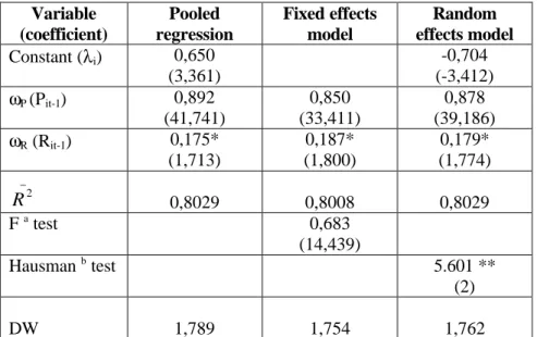
Table 3 reports the results regarding the estimation of equation (35).

Table 3 – Estimation of equation (35), dependent variable: primary surplus as a percentage of GDP (S) Variable (coefficient) Pooled regression Fixed effects model Random effects model Constant (βi) -0,390 (-2,488) -0,704 (-3,412) δ (Sit-1) 0,885 (39,363) 0,792 (29,870) 0,839 (34,338) θ (Bit-1) 0,011 (4,556) 0,030 (7,969) 0,019 (6,305) _ 2 R 0,7784 0,7950 0,7723 F a _{test 3,406*} (14,428) Hausman b _{test 27.159 **} (2) DW 1,759 1,766 1,616

The t statistics are in parentheses.

a - The degrees of freedom for the F statistic are in parentheses; the statistic tests the fixed effects model against the pooled regression model, where the autonomous term is the same for all countries, which is the null hypothesis.

b - The statistic has a Chi-square distribution (the degrees of freedom are in parentheses); the Hausman statistic tests the fixed effects model against the random effects, which is here the null hypothesis.

* - Statistically significant at the 1 percent level, the null hypothesis of the pooled regression model is rejected.

** - Statistically significant at the 1 per cent level, the null hypothesis is rejected (random effects model), that is, one rejects the hypothesis that the autonomous terms in each country is not correlated with the independent explanatory variables (in this case the random effects model does not produce unbiased and consistent estimators).

Notice that one can not reject the hypothesis θ > 0, since this coefficient is indeed

statistically different from zero and positive. In other words, the EU-15 governments seem to act in accordance with the existing stock of public debt, by increasing the budget surplus as a result of increases in the outstanding stock of public debt. This is also consistent with a Ricardian regime, where fiscal policy adjusts to the intertemporal budget constraint, preventing for that reason the determination of the price level through the budget constraint.

Table 3 reports also the results for the random effects model. The feasibility of the random effects model is assessed by the Hausman statistic, which tests the null hypothesis that the random effects are not correlated with the explanatory variables. In our case, and taking into account the fact that the test statistic is significant at the 1 per cent level, the random effects model hypothesis is rejected, in favour of the fixed effects model.

Additionally, one may also try to estimate the following model

it it it i it

S

B

v

B

=

α

+

γ

+

ϕ

+

where S is the primary surplus as a percentage of GDP, B is the debt-to-GDP ratio, the

index i denotes the country, the index t indicates the period and αi stands for the

individual effects to be estimated for each country i. One may then put forward the following ideas:

i) the hypothesis of a Ricardian regime, of monetary dominance, is not rejected

when γ < 0, most likely the government is using budget surpluses to reduce

outstanding public debt;

ii) with γ ≥0, there might be a non-Ricardian regime, that is, a regime of fiscal

dominance.

Table 4 presents the estimation results of equation (36). The possibility of the fixed effects model seems to get more statistical validation as one may confirm by the value of the F statistic. This is a test of the null hypothesis that all effects are the same for

each country, in other words, the hypothesis that all autonomous terms αi for equation

(36) are identical.25

25

The F statistic is computed as F (n-1, nT-n-k)=[(Ru 2 -Rp 2 )/(1- Ru 2 )][(nT-n-k)/(n-1)], where u stands

for the model without restrictions, p denotes the pooled regression, that is the model with the restriction that there is only one autonomous term, n is the number of countries, T is the number of periods and k is the number of exogenous variables (see for instance, Greene (1997) and Johnston and DiNardo (1997)).

Table 4 – Estimation of equation (36), dependent variable: debt-to-GDP ratio (B) Variable (coefficient) Pooled regression Fixed effects model Random effects model Constant (αi) 2,456 (7,124) 2,552 (5,387) γ (Sit-1) -0,618 (-12,469) -0,766 (-13,205) -0,716 (-13,287) ϕ (Bit-1) 0,987 (177,643) 0,989 (121,907) 0,988 (144,211) _ 2 R 0,9862 0,9874 0,9860 F a test 3,904* (14,429) Hausman b test 7.930 ** (2) DW 1,049 1,241 1,066

The t statistics are in parentheses.

a - The degrees of freedom for the F statistic are in parentheses; the statistic tests the fixed effects model against the pooled regression model, where the autonomous term is the same for all countries, which is the null hypothesis.

b - The statistic has a Chi-square distribution (the degrees of freedom are in parentheses); the Hausman statistic tests the fixed effects model against the random effects, which is here the null hypothesis.

* - Statistically significant at the 1 percent level, the null hypothesis of the pooled regression model is rejected.

** - Statistically significant at the 1 per cent level, the null hypothesis is rejected (random effects model), that is, one rejects the hypothesis that the autonomous terms in each country is not correlated with the independent explanatory variables (in this case the random effects model does not produce unbiased and consistent estimators).

From the results presented above one may see that there is some evidence in favour of a Ricardian regime, of monetary dominance, and that the EU-15 governments have a tendency to use primary budget surplus to reduce the debt-to-GDP ratio, since we get a

negative sign for the estimated γ coefficient (-0,766, in the fixed effects model) for

equation (36). There is therefore no evidence that can be regarded as supporting the FTPL for this set of European countries.

The fixed effects model is a typical choice for macroeconomists, and may eventually be more adequate than the random effects model. For instance, if the individual effects are somehow a substitute for non-specified variables, it is probable that each country specific effects are correlated with the other independent variables. In addition, and since the country sample includes all the relevant countries, the EU-15 countries, it is

less obvious that one might want to consider this set of countries as a random sample of a larger universe of countries.

In other words, and as reminded by Greene (1997) and Judson and Owen (1997), when the individual observations sample (countries in our case) comes from a larger population (which could be instance all the developed countries), it would be suitable to consider the specific constant terms as randomly distributed through the cross section units. However, and even if the present country sample includes a small number of countries, it is sensible to admit that the EU-15 countries have similar specific characteristics, not shared by the other countries in the world. In this case, it would seem adequate to choose the fixed effects formalization, even if it is not correct to generalize the results afterwards, to the entire population, which is not the purpose of the paper.

In the previous specification there is nevertheless an implicit assumption that the underlying model is homogeneous that is, the coefficients are the same for all countries. As a matter of fact, one of the problems with panel data estimations, as mentioned namely by Haque, Pesaran and Shrama (2000), is the possibility of the real model might be heterogeneous, with different coefficients for the explanatory variables in the cross-section dimension. Assuming the same coefficients for all the countries, with the exception of the intercept, may give rise to non-linearity in the estimations, even if the relation between the variables is linear. An alternative estimator, proposed by Pesaran and Smith (1995), the mean group estimator, is based on the separate estimation of the coefficients for each cross-section unit, through the least squares method, and then computing the arithmetic mean of those coefficients. Still, this alternative procedure, does not allow for the hypothesis that some of the coefficients may indeed be the same for several countries.

Besides the problem mentioned above, and to circumvent the potential non-stationarity problem arising from the time-series dimension of the data, empirical models in the literature are usually estimated with the first differences of the variables. Even so, in

most cases this procedure does not fully solve the problem.26 Also, the alternative of using variables in first differences might not take into account the fact that there is a levels relation between the government budget balance and the stock of outstanding public debt, through the present value borrowing constraint.

Another version of equation (36) was therefore estimated, using the first differences of the original variables

it it it i it

x

ks

wb

b

=

+

+

+

ϖ

where xi gives now the individual effects for each country i, and bit=Bit-Bit-1 and sit=Sit

-Sit-1.

Table 5 – Estimation of equation (37), dependent variable: first difference of the debt-to-GDP ratio (b) Variable (coefficient) Pooled regression Fixed effects model Random effects model Constant (xi) 0,396 (2,145) 0,398 (2,057) k (sit-1) -0,339 (-3,543) -0,360 (-3,708) -0,346 (-3,645) w (bit-1) 0,594 (15,299) 0,567 (13,708) 0,586 (15,103) _ 2 R 0,4077 0,3963 0,4077 F a _{test 0,460} (14,413) Hausman b _{test 2,557} (2) DW 2,083 2,068 2,068

The t statistics are in parentheses.

a - The degrees of freedom for the F statistic are in parentheses; the statistic tests the fixed effects model against the pooled regression model, where the autonomous term is the same for all countries, which is the null hypothesis.

b - The statistic has a Chi-square distribution (the degrees of freedom are in parentheses); the Hausman statistic tests the fixed effects model against the random effects, which is here the null hypothesis.

26 _{Some papers dealing with the properties of estimators, and recent developments in panel unit root}

tests and cointegration tests in panel data models are, for example, Alvarez and Arellano (1998), Phillips and Moon (2000) and Arellano and Honoré (2001).