Universidade de Lisboa
Faculdade de Ciências
Departamento de Estatística e Investigação Operacional
DOPPLER FLOW PATTERN IN PATIENTS WITH
AORTIC COARCTATION
Susana Cristina Oliveira Cordeiro
Dissertação orientada por
Prof. João Gomes e Dr. Rui Anjos
Mestrado em Bioestatística
i
Acknowledgements
To my mentor Rui Anjos, my greatest teacher in Pediatric Cardiology, I owe the idea and motivation for this dissertation.
To my mentor João Gomes, I am grateful for all the patience and time spent in answering all my questions. And for making his aim for all his students to use statistical theory as practical knowledge.
To all the Biostatistic course teachers, thank you for always being available to support students.
To my family, and particularly to my husband, a big appreciation for keeping me on the right track.
iii
Abstract
Patients with coarctation of the aorta (CoAo) often show a Doppler flow pattern with diastolic flow in the descending aorta. The effect of arterial stiffness on CoAo flow pattern was described in-vitro and with computer models. Study of Doppler flow patterns may provide helpful data to support the decision of CoAo treatment. Fifty studies were obtained in 31 patients (14 women, 21.5±15.5 years of age). In 19 patients, studies were performed before and after intervention. Systolic invasive gradients were measured (Sgrad). Doppler parameters measured at the time of invasive evaluation, included Doppler corrected gradient (Dgrad), diastolic velocity at end of T wave (DVT), end diastolic velocity (DVQ), systolic and diastolic half pressure times (SHPTc and DHPTc) and velocity runoff (VRc). Arterial stiffness was assessed by measuring pulsed wave velocity (PWV) between right carotid and radial arteries.
With simple regression models, Sgrad showed correlation with Dgrad, DVT, DVQ, SHPTc, DHPTc and VRc (p<0.01). The best multiple linear regression model provided the formula Sgrad = −4.61 + 0.75 × Dgrad + 0.06 × DHPTc (R2=0.77). A
binary variable named Sign were Sign=0 if Sgrad<20 mmHg and Sign=1 if Sgrad≥20 mmHg was created. The best multiple logistic regression model provided the formula 𝐿𝑛( 𝑝𝑆𝑖𝑔𝑛
1−𝑝𝑆𝑖𝑔𝑛)= −4.70 + 0.12 × Dgrad + 0.06 × DHPTc − 0.0008 × Dgrad ×
DHTPc. A cutoff value of 0.34 for 𝐿𝑛( 𝑝𝑆𝑖𝑔𝑛
1−𝑝𝑆𝑖𝑔𝑛) resulted in a sensibility of 96% and
specificity of 74% for this model.
A variable named DTail was obtained with DTail=0 if DHPTc=0 and DTail=1 if DHPTc>0. In the group with Sgrad below 30mmHg, a negative correlation was found between DTail and PWV (p=0.05) suggesting that low aortic stiffness may contribute to persistent diastolic flow in the descending aorta.
Doppler systolic and diastolic parameters correlated well with severity of CoAo. In mild to moderate CoAo, Doppler diastolic flow in the descending aorta was more likely in patients with lower arterial stiffness.
v
Resumo
A coartação da aorta (CoAo) é uma cardiopatia congénita caracterizada pelo estreitamento de um segmento da aorta torácica ou abdominal, mais frequentemente localizada no istmo aórtico. O Doppler codificado a cor e o Doppler espectral são ferramentas utilizadas no ecocardiograma transtorácico de rotina que permitem a avaliação do fluxo sanguíneo na aorta descendente. Em pessoas sem cardiopatia, o padrão de fluxo Doppler na aorta descendente apresenta uma velocidade máxima inferior a 2 metros por segundo e o fluxo ocorre apenas em sístole. Em doentes com CoAo, o padrão de fluxo Doppler apresenta um aumento da velocidade de fluxo sanguínea na aorta descendente e, em alguns casos, exibe uma persistência de fluxo em diástole, denominada extensão diastólica.
A gravidade da doença tem sido avaliada de forma invasiva, semi-invasiva ou com técnicas mais complexas, estudando a relação entre o diâmetro da CoAo e o diâmetro da aorta ao nível do diafragma (CoAo/DAo). No estudo de Carvalho et al. (1990), que utilizou a variável CoAo/DAo calculada por angiografia como referência padrão de gravidade da doença, o estudo por Doppler demonstrou ser mais eficaz em avaliar a gravidade da CoAo quando as quantificações Doppler sistólicas e diastólicas foram consideradas em conjunto. No estudo de Tan et al. (2005), utilizando a variável CoAo/DAo obtida por ressonância magnética e estudos Doppler antes e após implantação de stent, a velocidade de fluxo Doppler diastólica na onda T permitiu prever a gravidade da CoAo. Apesar da relação entre quantificações diastólicas do padrão de fluxo Doppler e a gravidade da CoAo ter sido descrita anteriormente, estudos prévios não utilizaram os gradientes invasivos.
Inicialmente pensou-se que a persistência de fluxo em diástole na aorta descendente de doentes com CoAo dependia apenas da gravidade da CoAo. Estudos prévios in-vitro (Tacy et al., 1999) e com modelos computacionais (DeGroff et al., 2003) sugeriram que a rigidez arterial deve ser considerada na avaliação de doentes com CoAo, visto que a extensão diastólica aumenta quando a rigidez arterial diminui.
vi
Assim, é objetivo desta dissertação descrever a relação entre o padrão de fluxo Doppler da CoAo, os gradientes invasivos da CoAo e a rigidez arterial, num grupo selecionado de doentes, utilizando modelos de regressão.
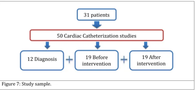
Cinquenta estudos foram obtidos em 31 doentes (14 mulheres, 21.5±15.5 anos de idade). Em 19 doentes, foram realizadas avaliações antes e após intervenção percutânea (dilatação com balão e/ou implantação de stent). Nos 50 estudos obtidos, 12 foram apenas de diagnóstico, 19 foram prévios à intervenção percutânea e 19 foram obtidos após a intervenção percutânea. Foram medidos os gradientes sistólicos invasivos (Sgrad) no cateterismo cardíaco. Por ecocardiograma transtorácico foram avaliados vários parâmetros de Doppler obtidos na altura do procedimento invasivo, que incluíram o gradiente de Doppler corrigido (Dgrad), a velocidade diastólica no final da onda T (DVT), a velocidade em telediástole (DVQ), os tempos de hemipressão sistólicos e diastólicos (SHPTc e DHPTc) e a velocidade runoff (VRc – tempo para a velocidade decrescer do seu valor máximo até 33%). VRc, SHPTc e DHPTc foram corrigidos com a fórmula de Bazett para normalizar as medições de tempos para diferentes valores de frequência cardíaca. A rigidez arterial foi estimada através da medição da velocidade da onda de pulso (PWV - pulse wave velocity) entre as artérias carótida e radial direita, por tonometria.
Através de regressão linear simples, Sgrad apresentou relação com Dgrad, DVT, DVQ, SHPTc, DHPTc e VRc (p<0.01). O modelo de regressão linear múltipla foi obtido, resultando na formula Sgrad = −4.61 + 0.75 × Dgrad + 0.06 × DHPTc. Apesar de Dgrad ter como objetivo estiar o valor que Sgrad por ecocardiografia, o modelo de regressão linear múltipla demonstrou que as variáveis que devem ser utilizadas para prever Sgrad são Dgrad e DHPTc. Este modelo apresentou um melhor ajustamento aos dados comparando com o modelo que inclui apenas a variável Dgrad (R2 = 0.77 incluindo Dgrad e DHPTc versus R2 = 0.74 incluindo
apenas Dgrad), demonstrando que DHPTc resolve parte da imprecisão de Dgrad em prever Sgrad.
Foi criada uma variável binária Sign onde Sign = 0 se Sgrad apresentasse valores inferiores a 20 mmHg e Sign = 1 se Sgrad apresentasse valores iguais ou superiores a 20 mmHg. O modelo de regressão logística múltipla foi obtido, resultando na
vii formula 𝐿𝑛 ( 𝑝𝑆𝑖𝑔𝑛
1−𝑝𝑆𝑖𝑔𝑛) = −4.70 + 0.12 × Dgrad + 0.06 × DHPTc − 0.0008 ×
Dgrad × DHTPc. Porque a consequência de uma CoAo não tratada tem um impacto significativo na saúde do doente, foi escolhido o cutoff de 0.34 para 𝐿𝑛 ( 𝑝𝑆𝑖𝑔𝑛
1−𝑝𝑆𝑖𝑔𝑛) que resultou em 96% de sensibilidade e 74% de especificidade para
este modelo, ou seja apenas 4% de falsos negativos e 26% de falsos positivos. Para os doentes identificados como falsos positivos no modelo de regressão logística proposto, a consequência é apenas a realização de um cateterismo de diagnóstico que tem baixa probabilidade de complicações.
Os estudos prévios que demonstraram o efeito da rigidez arterial no padrão de fluxo Doppler simularam esse efeito para CoAo com o mesmo grau de severidade. Posto isto, foi estudada a relação de PWV com as restantes variáveis na amostra inteira e em grupos selecionados de doentes. Como esperado, não foi encontrada relação significativa entre PWV e as restantes variáveis nos 28 doentes em que foi obtida medição de PWV (em 22 doentes não foi obtida medição de PWV). Através de análise gráfica, o grupo com Sgrad inferior a 30 mmHg foi selecionado (19 doentes). Para avaliar a relação entre PWV e DHPTc neste grupo, foi obtida uma nova variável DTail com DTail = 0 se DHPTc fosse também igual a zero e DTail = 1 se DHPTc apresentasse valores superiores a zero. Neste grupo com Sgrad inferior a 30 mmHg, verificou-se uma correlação negativa entre DTail e PWV através do modelo de regressão logística com a formula 𝐿𝑛 ( 𝑝𝐷𝑇𝑎𝑖𝑙
1−𝑝𝐷𝑇𝑎𝑖𝑙) = 6.69 − 0.94 × PWV,
com p=0.05 para o teste da razão de verosimilhanças. Este modelo prevê que para cada redução de 1 metro por segundo da PWV, existe uma probabilidade 2.57 vezes maior para DTail = 1, no grupo de doentes com Sgrad inferior a 30 mmHg. Este achado é concordante com os estudos prévios in-vitro e com modelos computacionais. Uma artéria com menor rigidez aumenta de diâmetro quando a onda de pulso a atravessa e depois regressa ao diâmetro basal. Na presença de CoAo, este retorno ao diâmetro basal no início da diástole pode ser o responsável pelo fluxo sanguíneo tardio que resulta na extensão diastólica. Por outro lado, uma artéria com maior rigidez não sofre o aumento de diâmetro fisiológico quando a onda de pulso a atravessa. Assim, a ausência de extensão diastólica em doentes com CoAo significativa pode ser devido a uma rigidez arterial aumentada. A
viii
relação significativa entre PWV e DTail sugere que a rigidez arterial reduzida pode contribuir para persistência de fluxo em diástole, sobretudo em doentes com CoAo ligeira ou moderada. Em doentes com CoAo grave, o obstáculo significativo parece induzir per se a presença de extensão diastólica, seja o PWV baixo ou elevado.
Em suma, Dgrad e DHPTc são variáveis obtidas por Doppler espectral no ecocardiograma que podem ser utilizadas para prever o gradiente invasivo da CoAo, Sgrad. Em doentes com CoAo ligeira a moderada, a rigidez arterial parece influenciar o valor de DHPTc visto valores mais elevados de DHPTc serem mais prováveis em doentes com menor rigidez arterial. Estes resultados foram obtidos pela aplicação de modelos de regressão que permitiram construir fórmulas matemáticas que podem ser utilizadas ao estudar os doentes com CoAo.
ix
Contents
List of Abbreviations ... xi
List of Figures ... xiii
List of Tables ... xv
Preface ... xvii
1 Biological Background ... 1
1.1 Coarctation of the aorta ... 1
1.1.1 Morphology... 1 1.1.2 Pathophysiology ... 3 1.1.3 Diagnosis ... 3 1.1.4 Treatment options ... 5 1.2 Arterial Stiffness ... 6 2 Statistical background ... 9 2.1 Linear Regression ... 9
2.1.1 Simple linear regression ... 9
2.1.2 Multiple linear regression ... 13
2.2 Logistic Regression ... 17
2.2.1 Simple logistic regression ... 17
2.2.2 Multiple logistic regression... 19
3 Methods and Results ... 21
3.1 Invasive Gradients... 25
3.2 Arterial Stiffness... 34
4 Discussion ... 39
References... 45
xi
List of Abbreviations
AIC Akaike’s Information Criterion ANOVA Analysis of Variance
BLUE Best linear unbiased estimator CoAo Coarctation of the aorta
CHD Congenital heart disease Dgrad Doppler corrected gradient
DHPTc Diastolic half pressure time, corrected with Bazett’s formula DVQ Diastolic velocity at Q wave
DVT Diastolic velocity at the end of T wave DTail Diastolic tail
OR Odds ratio
PWV Pulsed wave velocity
ROC Receiver Operating Characteristic Sgrad Systolic invasive gradients
Sign Significant invasive gradient
SHPTc Systolic half pressure time, corrected with Bazett’s formula TTE Transthoracic echocardiogram
VIF Variance inflation factor
VRc Velocity runoff, corrected with Bazett’s formula 2D Two-dimensional
xiii
List of Figures
Figure 1 Normal aortic arch (left) and aortic arch with CoAo (right). Figure 2 Color Doppler (left) and spectral Doppler (right) in CoAo.
Figure 3 Treatment options for CoAo: surgery (left), balloon dilatation (middle) and stenting (right).
Figure 4 Difference of blood flow velocity in compliant (left) and stiff (right) arteries.
Figure 5 Possible plots of the residuals. The horizontal line marks the zero. The top left plot shows Normal distribution of the residuals. The top 3 plots are all of homoscedastic residuals, but the middle and right are biased residuals. The bottom 3 plots are all of heteroscedastic residuals, but only the left is unbiased.
Figure 6 𝜇
𝑥 has a logistic function (left) and 𝐿𝑛 ( 𝑝𝑥
1−𝑝𝑥) is linear with 𝑥 (right).
Figure 7 Study sample.
Figure 8 Method used for measuring the PWV with tonometry.
Figure 9 Scatter plot analysis between Sgrad and the different TTE variables. The black lines correspond to the regression line for the simple linear regression models. The black dots in the VRc plot represent the simple regression model for Sgrad above and below 30 mmHg.
Figure 10 Best multiple regression model for the dependent variable Sgrad, obtained with R software.
xiv
Figure 12 Scatter plot (left) and Normal Q-Q plot (right) of the residuals. Figure 13 Scatter plot analysis between Sign and the different TTE variables.
Notice that all patients with DVQ superior to zero had Sign = 1.
Figure 14 Best logistic multiple regression model for odds ratio of the dependent variable Sign, obtained with R software.
Figure 15 Sensibility and specificity curves of the multiple logistic model. Figure 16 ROC curve of the multiple logistic model.
Figure 17 Sensibility and specificity values for choosing the cutoff of the model. Figure 18 Scatter plots between Sgrad and the TTE variables, Dgrad and DHPTc.
In the group of patients with Sgrad bellow 30 mmHg (horizontal line in the left plot), patients with higher PWV seem to have lower values of DHPTc. The black dots are from patients without measurement of PWV (missing data).
Figure 19 Scatter plot between Sgrad DHPTc, in the group of patients with Sgrad bellow 30 mmHg. Patients with higher PWV seem to have lower values of DHPTc. The black dots are from patients without measurement of PWV (missing data).
Figure 20 Boxplot between PWV and DTail, in the group with Sgrad bellow 30 mmHg.
Figure 21 Simple logistic regression model with DTail as the independent variable and PWV as the independent variable (top). OR of DTail for each unit of PWV (bottom).
xv
List of Tables
Table 1 ANOVA table with n the total of data, m groups being compared, SS the sum of squares where 𝑆𝑆𝑇𝑜𝑡 = 𝑆𝑆𝑅𝑒𝑔+ 𝑆𝑆𝐸 , Y the dependent variable, 𝑌̂ the estimator for Y, 𝑌̅ the mean of Y, 𝜀 the statistical error and i=1,…,n. Table 2 Variables included in the study.
xvii
Preface
Coarctation of the aorta (CoAo) is a congenital heart disease (CHD) characterized by the narrowing of a segment of the aorta. Color and spectral Doppler, tools used in standard routine echocardiography studies, allow for evaluation of blood flow in the aorta. In normal subjects, Doppler flow pattern in the descending aorta shows a peak velocity lower than 2 meters per second and flow occurs only during systole. In patients with CoAo, Doppler flow pattern shows an increased velocity in the descending aorta and, in some cases, a persistence of flow in diastole often referred as a diastolic tail. Color Doppler provides information of the narrowing site whereas spectral Doppler allows for quantitative analysis.
Previous studies have described a relation between CoAo Doppler flow pattern and CoAo severity. Using in-vitro and computer models, a relation between CoAo Doppler flow pattern and arterial compliance was demonstrated.
Carvalho et al. (1990) conducted a study where indices of severity of CoAo derived from non-invasive Doppler echocardiography were compared with measurements derived angiography. Using 24 studies from 17 patients, Doppler variables, including peak systolic and diastolic gradients and time to half peak systolic and diastolic velocities, were compared to a single angiography variable, ratio of CoAo diameter to the diameter of descending aorta at the level of diaphragm. A peak systolic gradient above 40 mmHg or time to half peak diastolic velocity above 100 ms were found to be highly specific for detecting an angiographic ratio below 0.5, with diastolic measurements more sensitive for diagnosis of severe coarctation than systolic measurements. They concluded that Doppler echocardiography was an effective non-invasive method of assessing severity of CoAo, particularly when systolic and diastolic events were considered together.
Another study conducted by Tan et al. (2005) focused on evaluating the effect of successful stenting on the CoAo Doppler flow pattern and identifying TTE indexes that could be used for follow-up. A TTE analysis before and after stenting included the variables peak systolic pressure gradient, diastolic velocity, end-diastolic tail velocity, systolic and diastolic velocity half-time index, systolic and diastolic
xviii
pressure half-time index. All TTE variables were compared to a single value for CoAo severity evaluation, the CoAo index (defined by the ratio of the narrowest coarctation cross-sectional area to the area of the abdominal aorta at diaphragm level) measured by magnetic resonance imaging. Diastolic velocity above 193 centimeters per second and a diastolic/systolic velocity ratio above 0.53 were highly predictive for a CoAo index below 0.25, and thus severe CoAo.
Using an in-vitro pulsatile flow model with four levels of CoA severity, Tacy et al. (1999) studied the relation between Doppler flow patterns at CoAo site and aortic compliance (calculated from local arterial stiffness). Diastolic runoff, defined as time between Vmax and 33% Vmax, had a positive linear relation with aortic compliance. They concluded that absence of a longer diastolic runoff in Doppler flow pattern should not exclude the diagnosis of significant CoAo.
In a computer model study, DeGroff et al. (2003) sought to investigate fluid and wall mechanics present in CoAo. They studied the relationship between diastolic runoff in Doppler flow pattern and aortic compliance (calculated from local arterial stiffness), using 3 computational numeric models of CoAo. In these simulations, the degree of diastolic runoff increased with arterial compliance. It was concluded that an increased aortic compliance induced greater dilatation and stored energy upstream the CoAo site in systole, with downstream release of the stored energy in diastole as the aortic wall recoils.
Although the relation between diastolic quantifications from the CoAo Doppler flow pattern and CoAo severity was already described, previous studies used variables obtained with the diameter of CoAo and not invasive gradients. But persistence of flow in diastole in the descending aorta of CoAo patients was thought to be solely dependent on lesion severity. Previous in-vitro and computer model studies suggested that arterial stiffness and compliance should be considered when evaluating a patient with CoAo, since the diastolic tail increases with decreasing arterial stiffness.
Therefore, this dissertation aims to describe the relation between CoAo Doppler flow pattern, CoAo invasive gradients and arterial stiffness, in a group of selected patients, using regression models.
1
1 Biological Background
This section is meant to describe CoAo and the concept of arterial stiffness. It provides an overview of CoAo definition, morphology and pathophysiology, diagnosis and treatment options. The concept of arterial stiffness is also described in this chapter.
1.1 Coarctation of the aorta
CoAo, or aortic coarctation, refers to narrowing of a segment of the thoracic or abdominal aorta, but it is most commonly located to the aortic isthmus (juxtaductal CoAo). CoAo is the seventh most common form of CHD, occurring in approximately 5 to 7% of CHD patients (approximately 36 per 100 000 live births), more likely in males. In some patients, CoAo manifests soon after birth, whereas in others it manifests at an older age. Whether it is genetic, environmental or hemodynamic, no single cause for CoAo has been proven. Abnormal flow distribution during fetal life with decreased aortic flow has long been suspected and histologic studies have demonstrated ductal tissue circumferentially surrounding the juxtaductal portion of the aorta. The role of genetic factors is increasingly recognized, for example CoAo occurs in approximately 12% of patients with Turner syndrome. CoAo is commonly associated with bicuspid aortic valve, ventricular septal defect and almost every type of CHD, particularly left heart obstructive lesions. A high incidence of associated cardiac abnormalities suggests that CoAo is a more complex defect than isolated narrowing of the aorta. (Lai et al., 2009)
1.1.1 Morphology
A juxtaductal CoAo usually results from narrowing of the aortic isthmus, in the proximal descending aorta at the arterial duct insertion. Different morphologic CoAo patterns can be distinguished based on age at diagnosis. In fetus and infant CoAo, the distal transverse aortic arch between the left common carotid and left
2
subclavian arteries is often hypoplastic, the angle between the ascending aorta and transverse arch is acute, the aortic isthmus is diffusely hypoplastic, and the arterial duct is usually patent. In older children and adult CoAo, aortic arch hypoplasia is less common, the coarctation segment is usually discrete and collateral arteries bypassing the CoAo are common. Unrelated to the age at diagnosis, the CoAo segment is characterized by luminal narrowing due to thickening of intima and media layers, hypoplasia and/or tortuosity. The length of the stenotic segment varies and the proximal descending aorta immediately past the CoAo often exhibits post-stenotic dilation. (Lai et al., 2009)
The morphology of abdominal CoAo is different from juxtaductal CoAo in that the involved segment is often long, the involvement of the renal and mesenteric vessels is common and the aortic media is thickened. (Lai et al., 2009)
3
1.1.2 Pathophysiology
CoAo is usually well tolerated in the fetus because blood flow to the lower body and the placenta is supplied predominantly through the arterial duct. But narrowing of the aortic isthmus may result in diversion of blood flow from the aorta to the arterial duct and pulmonary artery. As a result, the right ventricle dilates whereas the left ventricle is pressure loaded, resulting in the ventricular size disproportion in the fetus. The hemodynamic burden imposed by severe CoAo manifests after birth as the foramen ovale closes and the arterial duct constricts and ultimately closes. As a result, the cardiac output and flow to the lower body must cross the narrow aortic segment. Under these conditions, systolic blood pressure in the upper body is increased. With no patent arterial duct, systolic blood pressure is low distal to the CoAo, clinically manifesting as reduced pulse amplitude in the femoral arteries. In the neonatal period, a patent arterial duct may be present, allowing right-to-left systolic flow from the main pulmonary artery to the descending aorta, providing adequate perfusion to the lower body and normal volume of the femoral pulse. In the absence of an associated cardiac lesion, oxygen saturation in the upper extremities is greater than that in the lower extremities, a phenomenon called differential cyanosis. Constriction and closure of the arterial duct in neonates with severe CoAo may also lead to left ventricular dysfunction. (Lai et al., 2009)
Later in life, during childhood or in adults, CoAo is usually diagnosed either due to a heart murmur, low pulse amplitude in the lower extremities or systemic hypertension. Multiple collateral vessels tend to develop between the high-pressure aortic branches proximal to the CoAo and the low-high-pressure distal to the CoAo. (Lai et al., 2009)
1.1.3 Diagnosis
Clinical diagnosis of CoAo usually rests on identifying a blood pressure difference between the upper and lower extremities, information that can be obtained by palpation of both radial and femoral arteries. If a substantial difference between the two is found, coarctation of the aorta should be suspected. In a patient without
4
cardiac disease, blood pressure should be the same in upper and lower extremities. If the systolic blood pressure is at least 20 mmHg higher in the arms when compared to the legs, it is very likely that the patient has CoAo. In neonates or infants, the signs of congestive cardiac failure may be also present. (Johnson & Moller, 2014)
Transthoracic Echocardiography (TTE) provides adequate diagnostic information in most CoAo cases. However, some patients may require other diagnostic modalities, such as magnetic resonance imaging, computed tomography or angiography (Lai et al., 2009).
The basic elements of a standard TTE study are two-dimensional (2D) images enhanced by Doppler, color Doppler and M-mode information in multiple imaging planes. The TTE is organized by acoustic “windows” from which the heart is examined. In pediatric echocardiography, a segmental approach should always be used to describe all of the major cardiovascular structures in sequence, allowing the imaging of any structural or functional CHD. Any laboratory performing a pediatric echocardiogram should have a written examination protocol that outlines the views to be obtained, the imaging modalities and the methods for recording. (Lai et al., 2009)
The main goals of echocardiographic examination in the setting of CoAo are: evaluation of heart situs and segmental cardiac anatomy; evaluation of aortic arch anatomy; color Doppler evaluation of the flow profile in the descending aorta; assessment of spectral Doppler flow pattern at the CoAo site; evaluation of flow in the arterial duct; evaluation of morphology, size and function of the ventricles, inflow and outflow; identification of associated anomalies (Lai et al., 2009). Cross-sectional images for evaluation of aortic arch anatomy, that reveal the narrowing site, are usually best obtained with the transducer positioned near the suprasternal notch. Color Doppler shows a turbulent signal at the CoAo site and spectral Doppler shows high-velocity flow to the descending aorta, sometimes with persistence of blood flow in diastole. In neonates, the diagnosis may be difficult due to the presence of the ductus arteriosus. (Johnson & Moller, 2014)
5
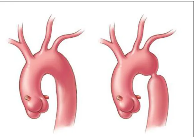
Figure 2: Color Doppler (left) and spectral Doppler (right) in CoAo.
Obtained by cardiac catheterization, an invasive diagnosis method, angiography is the gold standard imaging method for demonstrating the CoAo morphology. Invasive pressure measurements demonstrate systolic hypertension proximal to the coarctation and a gradient at the site of the coarctation, shown by pullback of the catheter across the lesion during pressure recording. (Johnson & Moller, 2014)
1.1.4 Treatment options
Treatment options for correction of CoAo include surgery, percutaneous balloon angioplasty and endovascular stent implantation. Surgery is the prefered treatment option for CoAo in neonates or for severe/complex CoAo anatomy in all patients. Balloon angioplasty and/or stent implantation are commonly used for treatment of CoAo in older children and adults. Balloon dilation of native coarctation avoids some surgery disadvantages but it is often less effective. Implantation of a metallic stent at the time of balloon dilation may provide better results but in small patients the stents do not allow for growth. Evaluation after surgery or transcatheter treatment of CoAo is similar to that of a native CoAo. Potential complications after treatment of CoAo that should be addressed include residual CoAo (immediately after treatment), recoarctation (development of narrowing after successful treatment), aneurysm formation, aortic dissection and persistent arterial hypertension. (Johnson & Moller, 2014)
6
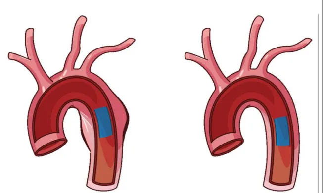
Figure 3: Treatment options for CoAo: surgery (left), balloon dilatation (middle) and stenting (right).
1.2 Arterial Stiffness
The mechanical behavior of the circulatory system is extremely complex. Arteries are known to have viscoelastic properties and powerful adaptive mechanisms. Arterial stiffness, and the opposite concept of arterial compliance, is related mainly to the viscoelastic properties of arteries. Local and regional arterial stiffness can be measured at various sites along the arterial tree. The downside is that elastic properties of arteries vary along the arterial tree. (Laurent et al., 2006)
Local arterial stiffness can be measured through high quality imaging methods, such as magnetic resonance imaging or computed tomography. Usually it is obtained by measuring the difference between the area or diameter of the artery in systole and in diastole. (Laurent et al., 2006)
Pulse wave velocity (PWV) is generally accepted as a simple, non-invasive and reproducible measurement to determine regional arterial stiffness. Carotid-femoral PWV has been used in epidemiological studies demonstrating the predictive value of aortic stiffness for cardiovascular events. (Laurent et al., 2006) Because compliant arteries suffer a small increase in diameter when the pulse wave passes through, this arterial wall motion absorbs some of the energy produced by the left ventricle in systole. This small and brief dilatation of the artery slows down the velocity of the pulse wave, but the propagation of the pulse
7 wave is more efficient due to arterial wall elasticity. Therefore, PWV is lower in more compliant arteries and higher in stiffer arteries (Figure 4).
9
2 Statistical background
This section is meant to describe theoretical knowledge for simple and multiple linear and logistic regression, explaining how to build regression models and how to evaluate them.
2.1 Linear Regression
In regression, when a variable Y is influenced by a variable X, Y is called the dependent variable and Xis the independent variable. If Y is a continuous variable, linear regression aims to represent the influence of one or more independent variables on Y through a straight line, called the regression line. (Oliveira, 2009)
2.1.1 Simple linear regression
In the particular case of simple linear regression, it is assumed that there is only the relationship between X and Y. Represented by Yx, each element of the
population is described by the values of X and Y. A linear regression model allows for the equation:
𝑌𝑥 = 𝜇𝑥+ 𝜀𝑥 = 𝛽0+ 𝛽1𝑥 + 𝜀𝑥 .
In this equation: 𝑌𝑥 is the dependent variable; μx is the mean value of the
dependent variable 𝑌𝑥 when the value for the independent variable X is 𝑥; 𝜀𝑥 is the
statistical error corresponding to possible unknown effects to 𝑌𝑥 beside the effect
of 𝑥; β0 is the mean value of the dependent variable when the independent variable
is equal to zero; β1 is the change in the mean value of 𝑌𝑥 for each unit of X. Hence, Y
answers to X trough a straight line (regression line) with origin in β0 and slope
equal to β1. The values for ε for the different elements in the population are not
related and should be independent by having a Gaussian probability distribution. (Gomes, 2011)
Assuming a random sample of size equal to n of a population Y with the characteristic X, ((𝑥1, 𝑌1),...,( 𝑥𝑛, 𝑌𝑛)), such as 𝑌𝑖 = 𝜇𝑖+ 𝜀𝑖 = 𝛽0+ 𝛽1𝑥𝑖+ 𝜀𝑖, with
10
of the regression model, β0 and β1, by the method of ordinary least squares or the
method of maximum-likelihood estimation. (Gomes, 2011)
The method of least squares is a standard approach to estimate β0 and β1, where
the regression line is obtained by defining the point where the variance of the distance of that point to all others is minimal (Oliveira, 2009). So, this method consists on finding the values that produce the minimum value of 𝑆𝑄 = ∑𝑛𝑖=1(𝑌𝑖− 𝛽0− 𝛽1𝑥𝑖)2 using the partial derivatives of SQ with respect to 𝛽0 and 𝛽1.
Another method for estimation of the parameters of the regression model is the
maximum-likelihood estimation. Through the assumptions defined earlier for
the population Y and 𝑌𝑖, we can conclude that (Y1,…Yn) is a vector of variables Yi
with Gaussian distribution with 𝜇𝑥 = 𝛽0+ 𝛽1𝑥 and 𝜎, the log-likelihood function is:
ln 𝐿 (𝛽0, 𝛽1, 𝜎2) = −𝑛
2ln(2π𝜎
2) − 1
2𝜎2∑ (𝑌𝑖− 𝛽0 − 𝛽1𝑥𝑖)2
𝑛
𝑖=1 . The estimators for β0
and β1 can be found by using the partial derivatives of ln 𝐿 with respect to 𝛽0 and
𝛽1. Both of these methods provide the estimator for β1 and β0 through the
formulas: 𝛽̂1= ∑ ( 𝑛 𝑖=1 𝑥𝑖− 𝑥̅)(𝑌𝑖− 𝑌̅) ∑𝑛𝑖=1(𝑥𝑖− 𝑥̅)2 and 𝛽̂0= 𝑌̅ − 𝛽̂1𝑥̅ .
The properties of these estimators stand that 𝛽̂1is an unbiased estimator for β1, as
𝛽̂0 is an unbiased estimator for β0. Both methods also provide the estimator for 𝜎2
through the formula: 𝜎̂2 = ∑ (𝑌
𝑖− 𝛽̂0− 𝛽̂1𝑥𝑖)2 𝑛
𝑖=1 / 𝑛 . (Gomes, 2011)
For testing the significance of the independent variable X, the test null hypothesis (H0) states that there is no significant alteration in the mean value of the
dependent variable Y when X changes (H0 : β1=0), were the alternative hypothesis
(H1) states that there is a significant alteration in the mean value of Y when X
changes (H1 : β1≠0 or β1>0 or β1<0). Analysis of Variance (ANOVA) table in used to
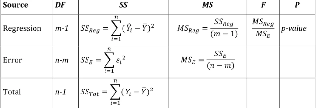
analyze the simple regression model. In an ANOVA table (Table 1), the column headings are usually “Source”, “DF”, “SS”, “MS”, “F” and “P”, were “Source” is the source of variation in the data (Regression, Error and Total), “DF” is the degrees of freedom in the source, “SS” is the sum of squares due to the source, “MS” is the
11 mean sum of squares, “F” is the test statistic F and “P” is the p-value for the F-test. (Pennsylvania State University, 2015)
Source DF SS MS F P Regression m-1 𝑆𝑆𝑅𝑒𝑔 = ∑( 𝑛 𝑖=1 𝑌̂𝑖− 𝑌̅)2 𝑀𝑆𝑅𝑒𝑔= 𝑆𝑆𝑅𝑒𝑔 (𝑚 − 1) 𝑀𝑆𝑅𝑒𝑔 𝑀𝑆𝐸 p-value Error n-m 𝑆𝑆𝐸= ∑ 𝜀𝑖2 𝑛 𝑖=1 𝑀𝑆𝐸 = 𝑆𝑆𝐸 (𝑛 − 𝑚) Total n-1 𝑆𝑆𝑇𝑜𝑡= ∑( 𝑛 𝑖=1 𝑌𝑖− 𝑌̅)2
Table 1: ANOVA table with n the total of data, m groups being compared, SS the sum of squares where 𝑆𝑆𝑇𝑜𝑡 = 𝑆𝑆𝑅𝑒𝑔+ 𝑆𝑆𝐸 , Y the dependent variable, 𝑌̂ the estimator for Y, 𝑌̅
the mean of Y, 𝜀 the statistical error and i=1,…,n.
Assuming the null hypothesis and with n-2 degrees of freedom in all simple regression models, the test statistic F has F distribution with parameters (1, n-2). With the level of significance of 100(1-α)%, it is also possible to obtain a
confidence interval for 𝛽1, through [𝛽̂1 − 𝑡(𝑛−2,𝛼 2)
𝑆𝛽̂1 , 𝛽̂1+ 𝑡(𝑛−2,𝛼 2)
𝑆𝛽̂1 ], with
𝑆𝛽̂1 = √∑𝑛 𝑀𝑆( 𝐸
𝑖=1𝑥𝑖−𝑥̅)2 . It is also possible to estimate the strength of the linear relation
between X and Y through the square of the sample correlation coefficient (square of 𝑟𝑋𝑌), called the determination coefficient (R2):
𝑅2 =𝑆𝑆𝑅𝑒𝑔 𝑆𝑆𝑇𝑜𝑡 = ∑𝑛𝑖=1(𝑌̂𝑖− 𝑌̅)2 ∑𝑛𝑖=1(𝑌𝑖− 𝑌̅)2 = [∑ (𝑥𝑖− 𝑥̅)( 𝑛 𝑖=1 𝑌𝑖− 𝑌̅)]2 ∑𝑛𝑖=1(𝑥𝑖− 𝑥̅)2∑𝑛𝑖=1(𝑌𝑖− 𝑌̅)2 = [𝑠𝑋𝑌 𝑠𝑋𝑠𝑌] 2 that assumes values within the interval [0,1], were R2≈1 means that there is a
perfect relation between X and Y while R2≈0 means that there is no relation.
(Gomes, 2011)
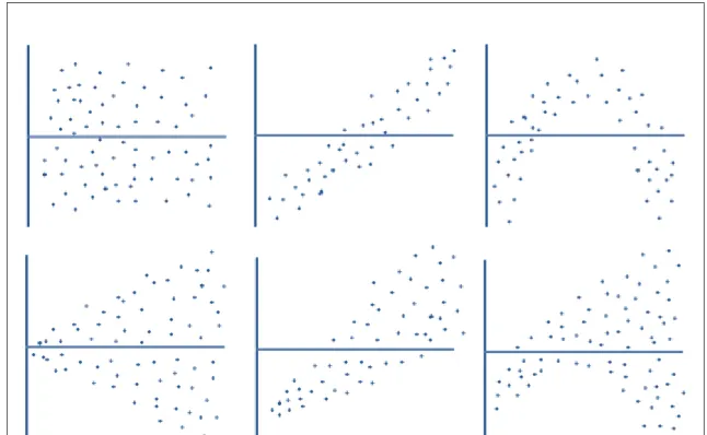
The residuals of the model should obey the Gauss Markov assumptions: the expected value is equal to zero for all observations (unbiased); conditional variance is a constant (homoscedasticity); have Normal distribution; the residuals are all uncorrelated. Verifying these assumptions can be performed by the analysis of the residuals, where a visual examination of the residuals plot alone provides indications of possible violation of the Gauss Markov assumptions (Figure 5).
12
Figure 5. Possible plots of the residuals. The horizontal line marks the zero. The top left plot shows Normal distribution of the residuals. The top 3 plots are all of homoscedastic residuals, but the middle and right are biased residuals. The bottom 3 plots are all of heteroscedastic residuals, but only the left is unbiased.
If the points in a residual plot are randomly dispersed around the horizontal axis with no particular pattern, a linear regression model is appropriate for the data because the residuals are homoscedastic (homogeneity of variance) and unbiased, otherwise a non-linear model is more appropriate. If the point in a residual plot are dominant in one side of the horizontal line marking the zero, this means that the distribution of the residuals is not normal. If the dispersion of the residuals is not constant and increase for greater values of the predicted values, this is called heteroscedasticity and may be corrected by changing the dependent variable (for example, using logarithm). When the residuals plot show a particular pattern, the residuals are biased, even if there is homoscedasticity. After a visual examination of the residuals plot, it is possible to test if the residuals have a normal distribution using, for example, the Kolmogorov-Smirnov test. (Oliveira, 2009)
13
2.1.2 Multiple linear regression
The aim for multiple linear regression is to find a linear equation that can predict the mean value of the dependent variable Y as a function of p independent variables Xj, with j=1,…,p. Considering an individual of the population with the
characteristics 𝐱 = (𝑥1, … , 𝑥𝑝), if there is a linear relation with the value associated to the characteristic Y (𝑌𝑥), that value can be described by the equation:
𝑌𝑥 = 𝜇𝑥+ 𝜀𝑥 = 𝛽0+ 𝛽1𝑥1+ 𝛽2𝑥2+ ⋯ + 𝛽𝑝𝑥𝑝+ 𝜀𝑥 .
In this model: 𝑌𝑥 is the dependent variable; 𝜇𝑥 is the mean value of the dependent variable; 𝛽0 is the mean value of the dependent variable when the value of all independent variable is equal to zero; 𝜀𝑥 is the statistical error corresponding to
possible unknown effects to 𝑌𝑥 beside the effect of x. The coefficients 𝛽𝑗 indicate the changes in the mean value 𝜇𝑥 for each unit of 𝑥𝑗, when all other variables 𝑥𝑗 are
constant. This model allows for accessing the marginal effect for each variable 𝑥𝑗 in
𝜇𝑥. (Gomes, 2011)
Assuming a sample of size equal to n of a population Y with the characteristic X where 𝜀𝑖⋂ 𝑁(0, 𝜎), 𝑌𝑖⋂ 𝑁( 𝜇𝑖, 𝜎) and 𝐸(𝜀𝑖𝜀𝑗) = 0 (i≠j), then:
𝑌𝑖 = 𝜇𝑖+ 𝜀𝑖= 𝛽0 + 𝛽1𝑥𝑖1+ ⋯ + 𝛽𝑝𝑥𝑖𝑝+ 𝜀𝑖, with i=1,…,n or in the matrix form:
𝐘 = 𝐗𝛃 + 𝛆 , where 𝐘 = [ 𝑌1 ⋮ ⋮ 𝑌𝑛 ] , 𝐗 = [ 1 𝑥11 ⋮ 𝑥21 … 𝑥1𝑝 ⋮ 𝑥2𝑝 ⋮ ⋮ 1 𝑥𝑛1 ⋮ ⋮ … 𝑥𝑛𝑝 ] , 𝛆 = [ 𝜀1 ⋮ ⋮ 𝜀𝑛 ] and 𝐸(𝐘) = 𝐗𝛃 .
Similar to the simple linear regression, both methods of ordinary least squares and of maximum-likelihood estimation provide the same estimators for the vector 𝛃. When estimating the parameters of the model, vector 𝛃 = (𝛽0, … , 𝛽𝑝), the method of least squares consists on finding the values that produce the minimum value of 𝑆𝑄(𝛽0, 𝛽1, … , 𝛽𝑝) = ∑𝑛𝑖=1𝜀𝑖2 = ∑𝑖=1𝑛 (𝑌𝑖− 𝛽0− 𝛽1𝑥𝑖1− ⋯ − 𝛽𝑝𝑥𝑖𝑝)2, or in
the matrix form 𝑆𝑄(𝛃) = 𝜀𝑇𝜀 = (𝐘 − 𝐗𝛃)𝑇(𝐘 − 𝐗𝛃), by using the partial derivatives
of SQ with respect to 𝛃. In the alternative maximum-likelihood estimation method, the aim is to maximize the log-likelihood function, 𝐿(𝛽0, … , 𝛽𝑝, 𝜎2) = ∏𝑛𝑖=1∅(𝑌𝑖−𝜇𝑖
𝜎 )/𝜎 , were ∅ is the probability density function of the reduced
14
the log-likelihood function using the partial derivatives of 𝑙(𝛃, 𝜎2) with respect to
𝛃. Both methods provide the formula:
𝛃̂ = (𝐗𝑇𝐗)−1𝐗𝑇𝐘 .
𝛃
̂ is a vector with (p+1) components. The mean value of 𝛃̂ is 𝛃 and the matrix of covariance of 𝛃̂, 𝐶𝑜𝑣(𝛃̂), is 𝜎2(𝐗𝑇𝐗)−1. (Gomes, 2011)
The ANOVA table can also be obtained for statistical inference of the multiple simple regression model (Table 1). 𝑀𝑆𝐸 = 𝑆𝑆𝐸
𝑛−𝑝−1 is a unbiased estimator for 𝜎 2. If 𝛽̂𝑗−𝛽1
√𝑀𝑆𝐸[(𝐗𝑇𝐗)−1]𝑗𝑖
∩ 𝑇𝑛−𝑝−1, with j=1,…,p and i=1,…,n, then the T-test of the coefficients states that there is significant change in the mean value of Y when X changes if
|𝛽̂𝑗| √𝑀𝑆𝐸[(𝐗𝑇𝐗)−1]𝑗𝑖
> 𝑡𝑛−𝑝−1;1−𝛼/2 . (Gomes, 2011)
If 𝛉 = 𝐂𝑇𝛃 is a linear combination of the elements of 𝛃, then 𝛉̂ = 𝐂𝑇𝛃̂ is a best
linear unbiased estimator (BLUE) according to the Gauss-Markov theorem . 𝛉̂ is a Gaussian vector with 𝐸(𝛉̂) = 𝐂𝛃 and 𝐶𝑜𝑣(𝛉̂) = 𝜎2𝐂(𝐗𝑇𝐗)−1𝐂𝑇. (Faraway, 2002)
If the aim is to test 𝐻0: 𝛉̂ = 𝐡 versus 𝐻1: 𝛉̂ ≠ 𝐡, one option is to use the test statistic:
𝐹 =(𝛉̂ − 𝐡)
𝑇(𝐂(𝐗𝑇𝐗)−1𝐂𝑇)−1(𝛉̂ − 𝐡)
𝑞 𝑀𝑆𝐸
Assuming 𝐻0, this test statistic has F distribution with parameters (q, n-p-1) and 𝐂 = [𝐜1𝑇, … , 𝐜𝑞𝑇] is the matrix with the linear combinations interesting to test. For
example, if the aim is to test if β1=0 and β2 + β3=0, then we have q=2, 𝐜1𝑇 =
[0 1 0 0 … 0] , 𝐜2𝑇 = [0 0 1 1 … 0] and 𝐡 = [00]. (Gomes, 2011)
As seen in the simple linear regression, the determination coefficient (R2) is
defined by 𝑅2 =∑𝑛𝑖=1(𝑌̂𝑖−𝑌̅)2 ∑𝑛𝑖=1(𝑌𝑖−𝑌̅)2 = 𝑆𝑆𝑅𝑒𝑔 𝑆𝑆𝑇𝑜𝑡 = 1 − 𝑆𝑆𝐸 𝑆𝑆𝑇𝑜𝑡 . But R
2 raises with the number of
parameters, not allowing a reliable information of the number of variables to include in the model. Therefore, R2 is often replaced by the adjusted-R2, or 𝑅
𝑎2, defined by: 𝑅𝑎2 = 1 − 𝑀𝑆𝐸 𝑀𝑆𝑇𝑜𝑡 = 1 −∑ ( 𝑛 𝑖=1 𝑌𝑖− 𝑌̂𝑖)2/(𝑛 − 𝑝 − 1) ∑𝑛𝑖=1(𝑌𝑖− 𝑌̅)2/(𝑛 − 1)
and whose name comes from the fact that it can be calculated using the same values for R2 adjusted with the respective degrees of freedom. (Gomes, 2011)
15 As a consequence of 𝛃̂, it is possible to find the predicted values 𝐘̂, corresponding to the values in the linear regression line, and find the residuals through 𝐞 = 𝐘 − 𝐘̂. The analysis of the residuals should be performed the same way as it was described in the simple linear regression model.
A multiple regression model should not have unnecessary independent variables and should have all significant independent variables to explain the variability of the dependent variable. Including unnecessary independent variables in the regression model may lead to imprecise estimators for the coefficients due to excessive fitting of the data, a problem called overfitting. On the other hand, by not including all significant independent variables, its effect on the dependent variable will be distributed on the other independent variables, biasing the coefficients. (Oliveira, 2009)
Selecting the variables according to the higher value of R2 always leads to the
choice of the complete model. Even when using the adjusted-R2, this correction is
still not enough and tends to select too many variables. If the model has less than the necessary independent variables, the estimator for 𝜎2 tends to be higher than
the complete model, therefore it is important to seek a model that has a small value for MSE. Backward elimination is a method of selecting the best subset of the
"complete model" (model with all independent variables) through eliminating one by one the independent variables with the higher p-values in the T-test until all variables included in the model have p-value lower than the chosen level of significance. Another method is to select the independent variables sequentially, evaluating the importance of each dependent variable by identified the model which produces the lowest value of MSE, called Forward selection. Bidirectional
elimination is a combination of the two methods. (Gomes, 2011)
In multiple regression, one independent variable should not be completely determined by one or several other independent variables, but it is also possible to violate this condition through the presence of multicollinearity. It is important to identify and also solve this problem without compromising the quality of the model. Sometimes, a simple analysis of the correlation matrix is enough to realize the presence of multicollinearity and which independent variables are correlated. (Oliveira, 2009) Another method for evaluating the presence of multicollinearity is
16
the term 1
1−𝑅2 , referred to as a variance inflation factor (VIF). The square root of
VIF explains how much larger the standard error is, compared with what it would be if that variables were uncorrelated. (Hsieh, 1998)
Another situation that can occur in multiple regression is interaction and
confounding, Interaction occurs when the effect of one independent variable on
the dependent variable is not the same for every values of another independent variable. For example, when studying the relation between different hospitals (dependent variable) and time form diagnosis to treatment, the CoAo severity may motivate different times. Confounding happens when adding an independent variable provides an alternative explanation for the relation between the dependent variable and another independent variable. For example, because in CoAo patients different ages require different treatments (Chapter 1.1.4), the patient’s age changes the relation between arterial hypertension (dependent variable) and type of treatment. These problems are difficult to recognize and the solution might be to remove the variable causing the problem or to build separate regression models (Oliveira, 2009).
17
2.2 Logistic Regression
Binary regression models are a consequence of a categorized dependent variable. Logistic regression model are a particular case of binary regression models where the dependent variable assumes only the values 0 and 1.
2.2.1 Simple logistic regression
Considering a regression model where the dependent variable 𝑌𝑥 has a Bernoulli
distribution, or 𝑌𝑥∩ 𝐵(𝑝𝑥), the probability mass function is 𝑃(𝑌𝑥 = 𝑦) = 𝑝𝑥𝑦(1 − 𝑝𝑥)1−𝑦, or 𝑌𝑥{
0 1 − 𝑝𝑥
1 𝑝𝑥 . For each element of this population, the simple logistic
model aims to find the constants 𝛽0 and 𝛽1 that resolve the formulas: 𝜇𝑥= 𝑝𝑥 = exp (𝛽0+𝛽1𝑥)
1+exp (𝛽0+𝛽1𝑥) and 𝐿𝑛 ( 𝑝𝑥
1−𝑝𝑥) = 𝛽0+ 𝛽1𝑥 (canonic link).
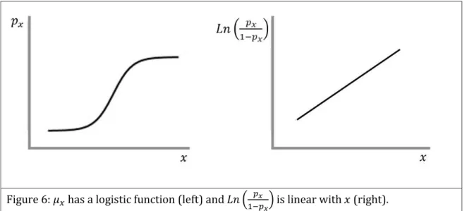
This means that 𝑝𝑥 has a logistic function and the logarithm of the odds, 𝐿𝑛 ( 𝑝𝑥
1−𝑝𝑥),
is linear with 𝑥 (Figure 6). (Gomes, 2011)
Figure 6: 𝜇𝑥 has a logistic function (left) and 𝐿𝑛 ( 𝑝𝑥
1−𝑝𝑥) is linear with 𝑥 (right).
The maximum-likelihood estimation method, used in linear regression aims to find the estimators for 𝛽0 and 𝛽1 that maximize the log-likelihood function defined by
the formula: 𝐿𝑛 𝐿 (𝒚, 𝒙) = ∑ 𝑙𝑖 = ∑[𝑦𝑖(𝛽0+ 𝛽1𝑥𝑖) − 𝐿𝑛 (1 + 𝑒𝑥𝑝(𝛽0+ 𝛽1𝑥𝑖))]. The estimators for β0 and β1 can be found by using the partial derivatives of the
log-18
likelihood function. Both of these methods provide the equation:
{ ∑ 𝜕𝑙𝑖 𝜕𝛽0 𝑛 𝑖=1 = ∑𝑛𝑖=1(𝑦𝑖− 𝑝𝑖) = 0 ∑ 𝜕𝑙𝑖 𝜕𝛽1 𝑛 𝑖=1 = ∑𝑛𝑖=1𝑥𝑖(𝑦𝑖− 𝑝𝑖) = 0
. Or in the matrix form: 𝐗𝑇(𝐘 − 𝐩) = 0 with Y and
𝐩 size nx1 matrixes and 𝐗𝑇 = [1 … 1
𝑥1 … 𝑥𝑛]. These equations do not have an
analytical solution, therefore in is necessary to use an iterative method. Considering a U function such as 𝑈(𝛽0, 𝛽1) =(∑ 𝜕𝑙𝑖
𝜕𝛽0 𝑛 𝑖=1 , ∑ 𝜕𝑙𝑖 𝜕𝛽1) 𝑇 𝑛 𝑖=1 , the
Newton-Raphson method can be applied. [−𝜕𝑈
𝜕𝛃] is the partial derivative matrix of U and it
can be replaced by 𝐗𝑇𝐖𝐗 with 𝐖 = 𝐷𝑖𝑎𝑔(𝐩(1-p)). This iterative method aims to
find the values of β0 and β1 where the U function is close to zero. With 𝛃 = (𝛽0, 𝛽1),
this can be obtained through the formula:
𝛃(𝑚+1)= 𝛃(𝑚)+ [𝐗𝑇𝐖𝐗]−1𝛃(𝑚)[𝐗𝑇(𝐘 − 𝐩)]𝛃−1(𝑚).
After finding the estimators for 𝛃, the analysis the logistic regression model should be performed. In logistic regression, the Deviance of a model is calculated by comparing the simple regression model (M) to the perfectly adjusted model (Ms)
or to the null model (M0) (Oliveira, 2009). Assuming L as the likelihood function,
the likelihood-ratio is calculated by 𝜆1= 𝐿(𝑀)
𝐿(𝑀𝑠) and the measurement of the
Deviance of M to Ms is calculated by 𝐺1 = −2𝐿𝑛(𝜆1). In the same way, assuming
𝜆0 =𝐿(𝑀0)
𝐿(𝑀𝑠) , the measurement of the Deviance of M0 to Ms is 𝐺0= −2𝐿𝑛(𝜆0). A
higher Deviance translates into a larger difference between the two model that are being compared. Because 𝜆0∩ 𝜒𝑛−12 and 𝜆1∩ 𝜒𝑛−22 , the value for 𝐺0− 𝐺1 can be
compared to the 𝜒12 quantil of chosen level of significance. This test is called the
likelihood-ratio test. (Gomes, 2011)
Other statistical tests can be used in evaluating the logistic regression model such as the Wald test, the Score test, the Hosmer-Lemeshow test. (Gomes, 2011)
In the case of a continuous independent variable and because the canonic link is the logarithm of the odds, it is possible to estimate the Odds Ratio (OR) for each unit of the independent variable through OR = exp (𝛽1). (Oliveira, 2009)
19 The Receiver Operating Characteristic (ROC) curve is used to evaluate the capacity of the model to discriminate between “Y=1” and “Y=0” and it is obtained using the sensibility and specificity curves. By means of choosing a cutoff value c, 𝑌̂ = 1 if the result for the odds is equal or higher than c. The sensibility of a model is the probability of correctly predicting “Y=1”, calculated by (𝑌̂ = 1|𝑌 = 1) =
𝑃(𝑌̂=1 ∩ 𝑌=1)
𝑃(𝑌=1) . The specificity of a model is the probability of correctly predicting
“Y=0”, calculated by 𝑃(𝑌̂ = 0|𝑌 = 0) =𝑃(𝑌̂=0 ∩ 𝑌=0)
𝑃(𝑌=0) . The probability of false
negatives can be calculated by 1 − 𝑃(𝑌̂ = 1|𝑌 = 1) and the probability of false positives can be calculated by 1 − 𝑃(𝑌̂ = 0|𝑌 = 0). Different cutoff values for the model provide different values of sensibility and specificity. (Gomes, 2011)
The area under the ROC curve measures the percentage of the data that is correctly categorized, therefore reflecting the performance of the model. Authors suggest that a logistic regression model should have an area under the ROC curve above 80% for the data to have clinical interest. (Oliveira, 2009)
2.2.2 Multiple logistic regression
A regression model with the dependent variable Y where 𝑌 ∩ 𝐵(𝑝) and 𝑌 {0 1 − 𝑝
1 𝑝 , but instead of one independent variable there are p independent variables, 𝐱 = (𝑥1, … , 𝑥𝑝), is a multiple logistic regression model. The mean value of Y conditional to x is E[𝑌𝑖|𝐱𝑖 = (𝑥𝑖1, … , 𝑥𝑖
𝑝
)] = 𝜇𝑖= 𝑝𝑥𝑖. Then, the formulas for the
multiple logistic regression are: 𝑝𝑥 =
exp (𝛽0+𝛽1𝑥1+⋯+𝛽𝑝𝑥𝑝)
1+exp (𝛽0+𝛽1𝑥1+⋯+𝛽𝑝𝑥𝑝) and 𝐿𝑛 (
𝑝𝑥
1−𝑝𝑥) = 𝛽0 + 𝛽1𝑥1+ ⋯ + 𝛽𝑝𝑥𝑝.
Similar to the simple logistic regression, the aim is to find the estimators for 𝛃 = (𝛽0, 𝛽1, … , 𝛽𝑝) that maximize the log-likelihood function, in this case defined by: 𝐿𝑛 𝐿 (𝒚, 𝒙) = ∑[𝑦𝑖(𝛽0+ 𝛽1𝑥1+ ⋯ + 𝛽𝑝𝑥𝑝) − 𝐿𝑛 (1 + 𝑒𝑥𝑝(𝛽0+ 𝛽1𝑥1+ ⋯ + 𝛽𝑝𝑥𝑝))]. This
method also results in 𝐗𝑇(𝐘 − 𝐩) = 0 with Y and 𝐩 size nx1 matrixes and 𝐗𝑇 a size
(p+1)xn matrix, which means no analytical solution. Using the iterative
20
obtained through the same formula explained in the simple logistic regression: 𝛃(𝑚+1)= 𝛃(𝑚)+ [𝐗𝑇𝐖𝐗]−1𝛃(𝑚)[𝐗𝑇(𝐘 − 𝐩)]𝛃−1(𝑚). (Gomes, 2011)
After finding the estimators for 𝛃, evaluation of the model can be made through a value that represents a relative measurement of the information lost in a particular model, called Akaike’s Information Criterion (AIC). With k parameters and L the likelihood of the model, this value can be calculated by AIC = −2[𝐿𝑛(𝐿) − 𝑘]. The best model should have low AIC. (Gomes, 2011)
To select the best set of variables for the multiple logistic regression model, it is necessary to first understand how each independent variable behaves in relation to the dependent variable (for example, using plot analysis). Then, an analysis of the importance of each independent variable should be performed, using a quantitative values such as the Deviance and likelihood-ratio test (see Chapter 2.2.1) and the value of AIC. Similar to the multiple linear regression, the selection of the best set of variables can be performed through backward elimination (best subset of the complete model), forward selection (selecting independent variables sequentially) or bidirectional elimination (combination of backward elimination and forward selection). (Gomes, 2011)
In multiple logistic regression, ROC curve analysis can also be used to evaluate the performance of the selected model model. (Oliveira, 2009)
21
3 Methods and Results
Our sample included 31 patients with CoAo that underwent cardiac catheterization in Santa Cruz Hospital. Native CoAo was found in 23 patients and 8 patients underwent previous intervention. Overall mean age was 21.5 years, form patients between 4 and 62 years old, and 14 were women. In 19 patients, data was obtained from before and after intervention (balloon dilatation and/or stenting). Therefore, 50 cardiac catheterization studies were included, 12 with only diagnostic data, 19 with data before percutaneous intervention and 19 with data after percutaneous intervention (Figure 7).
Figure 7: Study sample.
Because there was no significant modification to the patient’s aortic arch before or after cardiac catheterization, TTE and arterial stiffness studies performed within 45 days before or after were not excluded from the data. In the TTE studies associated to the diagnostic only cases and before intervention, 28 studies were performed the same day or the day before intervention and only 3 studies performed within 45 days before intervention. In the TTE studies associated to the data after the cardiac catheterization, 17 studies were preformed 1 day after intervention and only 2 studies performed within 45 days after intervention. Form the arterial stiffness studies associated to the diagnostic only cases and before intervention, 14 studies were performed the same day or the day before
19 After intervention 19 Before intervention 12 Diagnosis
50 Cardiac Catheterization studies 31 patients
22
intervention and only 2 studies were performed within 45 days before intervention. In the arterial stiffness studies associated to the data after cardiac catheterization, 11 studies were preformed 1 day after intervention and only 1 study was performed within 45 days after intervention. In total there were 28 arterial stiffness studies performed and, because there are 50 cardiac catheterization studies, 22 patients had missing data for the arterial stiffness study.
The variables included in the data were obtained by cardiac catheterization, TTE and arterial stiffness studies (Table 2).
Method Variables
Cardiac
Catheterization Sgrad – Systolic invasive gradient
TTE
Dgrad – Doppler corrected gradient
DVT - Diastolic velocity at the end of T wave DVQ - Diastolic velocity at Q wave
SHPTc - Systolic half pressure time DHPTc - Diastolic half pressure time VRc - Velocity runoff
Arterial
Stiffness PWV – Pulse wave velocity between right carotid and radial arteries Table 2. Variables included in the study.
In the cardiac catheterization, systolic invasive gradients were measured (Sgrad) with an invasive catheter and a Transpac® disposable pressure transducer.
TTE studies were all performed with the Vivid7® ultrasound machine from General Electric®. TTE variables included were obtained by measuring the Doppler corrected gradient (Dgrad), diastolic velocity at end of T wave (DVT), diastolic velocity at Q wave (DVQ), systolic and diastolic half pressure times (SHPTc and DHPTc) and velocity runoff (VRc). Doppler gradients are obtained through the Bernoulli’s formula were the gradient is equal to 4 times the squared
23 Doppler velocity, which reads ∆𝑝 = 𝑝1 − 𝑝2 = 4𝑣2. Dgrad was obtained by
subtracting the Doppler gradient before the CoAo site to the Doppler gradient after the CoAo site, measured in millimeters of mercury (mmHg). Both in meters per second (m/s), DVT as measured at the end of the electrocardiographic T wave, marking the beginning of the diastole, while DVQ was measured at the electrocardiographic Q wave, marking the end of the diastole. SHPTc was defined as the time for the maximum value of the Doppler gradient to decrease to half its value, while DHPTc was defined as the time for the Doppler gradient starting at the electrocardiographic T wave to decrease to half its value, both in milliseconds (ms). VRc was defined as the time for velocity to decrease from maximum value (Vmax) to 33% Vmax, in m/s. VRc, SHPTc and DHPTc were corrected with Bazett’s formula, where the time is divided by the squared root of the RR interval, which is calculated through the heart rate, to resolve the problem that different heart rates produce different time measurements in each cardiac cycle.
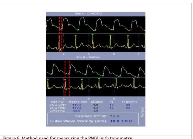
Arterial stiffness studies were assessed by tonometry, with the Sphygmocor® equipment, and the variable included in the data was obtained by measuring pulsed wave velocity (PWV). PWV was measured between right carotid and radial arteries, in order to avoid any influence that the CoAo obstruction may have in the left radial artery and in the femoral arteries. The method used for measuring the PWV (Figure 8) consists on subtracting the time between the electrocardiographic Q wave and the start of the carotid pulse wave (t1) to the time between the
electrocardiographic Q wave and the start of the radial pulse wave (t2), where ∆t =
t1 - t2. It is also necessary to subtract the distance between the sternal furcula and
the location of the radial pulse (d1) to the distance between the sternal furcula and
the location of the carotid pulse (d2), where ∆d = d1 - d2. Then, PWV is a velocity
24
Figure 8. Method used for measuring the PWV with tonometry.
Overall, mean Sgrad was 23.5 mmHg, mean Dgrad was 32.2 mmHg, mean DVT was 1.0 m/s, mean DVQ was 0.3 m/s, mean SHPTc 101.5 ms, mean DHPTc 70.1 ms, mean VR 368.7 ms and mean PWV was 7.18 m/s.
To describe the relation between CoAo Doppler flow pattern, CoAo invasive gradients and arterial stiffness, the results were divided into results for invasive gradients and results for arterial stiffness. In the results for invasive gradients, only the relation between CoAo Doppler flow pattern and CoAo invasive gradients was studied. In the results for arterial stiffness, the relation between CoAo Doppler flow pattern and arterial stiffness was studied. All statistical analysis was performed using R version 3.1.2 software.
25
3.1 Invasive Gradients
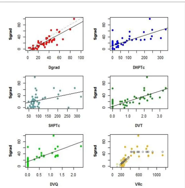
Scatter plot analysis between Sgrad and the different TTE variables was performed (Figure 9). All plots suggest a positive relation with Sgrad. The variables Dgrad and DHPTc seemed to have the best linear relation with Sgrad. Dgrad seems to slightly overestimate Sgrad. The variables SHPTc, DVT and DVQ also showed a positive relation with Sgrad. The variable VRc showed a better linear relation for Sgrad bellow 30 mmHg.
Figure 9: Scatter plot analysis between Sgrad and the different TTE variables. The black lines correspond to the regression line for the simple linear regression models. The black dots in the VRc plot represent the simple regression model for Sgrad above and below 30 mmHg.