1
Forecasting Industrial Production Index by its aggregated or
disaggregated data? Evidence from one important emerging market
economy
∗
Diogo de Prince
†Emerson Fernandes Marçal
‡Pedro Luiz Valls Pereira
§Abstract
Our work aims to address if the use of disaggregate data helps to forecasting industrial production index. We use Brazilian industrial production data and we investigate if disaggregate information improves the accuracy of the forecasts. We use a a number of recent econometric techniques such as the weighted lag adaptative least absolute shrinkage and selection operator (WLadaLASSO) methodology, the exponential smoothing (selecting the most appropriate model) and Autometrics algorithm to model both aggregates and disagregates. As far as we known this is the novelty of the work. We run a a forecasting exercise from one up to 12 months ahead for Brazilian industrial production. Our full sample covers the period from January of 2002 to August of 2017. Our results suggest that modeling disaggregate data better using exponential smoothing model provides the best performance for 1 up to 7 months ahead for Brazilian industrial production using mean square error as a metric and Autometrics algorithm provides better forecast for 8 up to 12 months but it is not clear whether aggregate or disagregate data is the best choice given that they are both part of the final set of good predictions. JEL Codes: C53, E27, C52
Key Words: industrial production, forecasting, model selection.
1 Introduction
Economic agents decide based on a global view of how the economy behaves at that moment and what are your expectations for the future. The general levels of output, employment, interest rates, exchange rates and inflation are examples of key economic indicators that help in the country’s diagnosis. Therefore, the proposition and evaluation of econometric models devoted to forecast bring benefits to build better guides to economic agents and policy makers. One of the most comprehensive and important macroeconomic indicators of the economy is the Gross Domestic Product (GDP), as it is a proxy for a country’s economic performance. In the present work, the proxy used for GDP is industrial production, since the indicator of industrial production is monthly (higher frequency than GDP) and is released with a lag of about one month, which is therefore smaller than GDP (with a delay of more than two months).
∗We thank seminar participants at Sao Paulo School of Economics and Anpec 2018 (Rio de Janeiro). The authors gratefully acknowledge financial support from CNPq. We also thank Eusebio Souza and Thais Beserra for the research assistance.
† Researcher of Center for Applied Macroeconomic Research and Assistant Professor at Federal University of Sao Paulo ‡ Lecturer at at Sao Paulo School of Economics and Head of Center for Applied Macroeconomic Research
2
A point to address is if the use of disaggregated data improves to forecast variables comparable to using ag- gregated series. Data disaggregation is an alternative to lead to more accurate forecasts. This alternative refers to the decomposition of the main variable into several subcomponents, which have different weights for the aggre- gate series. We estimate these subcomponents individually and then we grouped these subcomponents to obtain a forecast of the aggregate series. This technique can increase the quality of the forecast because we model the subcomponents taking into account their individual characteristics. We use this alternative in the present work to understand if there are gains to predict the aggregate series if we estimate each subcomponent and we use the weight of this subcomponent. Another alternative is to estimate using only lagged aggregate variable to forecast the aggregate series.
The accuracy of using disaggregated or aggregate data for forecasting has been discussed in some studies. The theoretical studies indicate that when the data generating process (DGP) is known, it is preferable to first use the disaggregated data in multiple series to later aggregate them than to directly predict the already aggregated series. However, the literature acknowledges that in most cases DGP is unknown and therefore the use of aggregate series may be preferable due to variability of specification and estimation of the model (because the estimation has fewer parameters). Some examples of contributions to the theoretical literature on aggregate or disaggregate forecasting are Lutkepohl (1984, 1987), Granger (1987), Pesaran, Pierse, and Kumar (1989), Garderen, Lee, and Pesaran (2000), and Giacomini and Granger (2004). As DGP is not known, then the question (if aggregating the disaggregated forecasts improves the accuracy of the aggregate forecast) becomes an empirical question.
Our point is whether the prediction of the disaggregated components of Brazilian industrial production improves the accuracy of the forecast of aggregate Brazilian industrial production. Our contribution is that we do not know articles that address the contribution of the disaggregated data of the weighted lag adaptative least absolute shrinkage and selection operator (WLadaLASSO) methodology or the exponential smoothing (selecting the most appropriate model). In addition, there are few papers that analyze the contribution of disaggregated data to forecast the industrial production and we intend to fill this gap. Using monthly data from 2002 to 2017, we select the best univariate model, we estimate a rolling window of 100 fixed observations and we evaluate the forecast from 1 to 12 months ahead for Brazilian industrial production, in which we estimate 61 rolling windows. We consider as naive models the first order autoregressive model (AR(1)), AR(1) with time-varying parameters (TVP AR(1)), and the Stock and Watson (2007) unobserved components with stochastic volatility (UC-SV) estimated based on Barnett et al (2014). We consider the following methods for selecting the best model: exponential smoothing based on Hyndman et al (2002), Hyndman and Khandakar (2008) and Hyndman et al (2008), the least absolute shrinkage and selection operator (LASSO), adaptive LASSO (adaLASSO), the WLadaLASSO and the Autometrics algorithm with break dummy variables. We use the LASSO and its variants to select the lags from an AR (15) and we consider the Autometrics algorithm to select break dummy variables in the sample and the lags from an AR(15). We compare the prediction performance between the models based on the mean square error (MSE), the Diebold and Mariano (1995) test and the Model Confidence set procedure of Hansen et al (2011).
Our results point to a better performance of the exponential smoothing model with disaggregated data for the forecast of 1 to 7 months ahead for Brazilian industrial production by MSE. But the Autometrics algorithm with step dummy variables (and considering a p-value of 0.1%) with the disaggregated forecasts has more accuracy for 10 to 12 months ahead by MSE. To analyze whether there is a better statistical performance, we use the exponential model with disaggregated data as a benchmark in the Diebold and Mariano (1995) test. We obtain that the disaggregated exponential smoothing model presents better forecast performance in relation to the naive models (AR(1), AR(1) with time-varying parameters, UC-SV) considered with aggregate or disaggregated data and the aggregate exponential smoothing model.
The article structure contains six sections in addition to this introduction. The following is a brief review of the literature. Next, we address the methodology of the models considered in the paper. Section 4 presents the
3
data used, the empirical forecasting strategy, the Diebold and Mariano (1995) test and the Model Confidence set to compare the performance of the models. In section 5, we discuss the results of the study. Finally, we show the final considerations of the research and the next steps.
2 Literature Review
This section presents some empirical articles that address the difference in forecast accuracy between aggregating the disaggregated forecasts or modeling only the aggregate variable. Stock and Watson (1998) compare 49 univariate projection models to forecast industrial activity and inflation in the United States from 215 monthly series from the years 1959 to 1996. One conclusion of the paper is that the forecast aggregation has better performance than separate forecasts. The authors also find signficant gains using forecast combinations and these gains are enough to justify their use by a risk-averse analyst. Stock and Watson (1998) also point to the importance of performing the unit root test to reduce errors substantially in the estimates. Tobias and Zellner (1998) seek to determine the effects of aggregation and disaggregation to predict the average annual growth rate of 18 countries. In general, the disaggregation leads to more observations to estimate the parameters, besides the authors obtain better predictions for the aggregate variable (growth rate).
Marcellino, Stock and Watson (2003) find evidence that the individual estimation of inflation in each euro area country and the subsequent aggregation of projections increases the accuracy of the final result of the estimation in relation to the option to forecast this variable only in aggregate level. Hubrich (2005) obtains that aggregating forecasts for each component of inflation does not necessarily better predict year-on-year inflation in the euro area one year ahead. Espasa, Senra and Albacete (2002) have similar results indicating, however, that the disaggregation leads to better projections for periods longer than one month. Carlos and Marï¿œal (2016) compare forecasts from models for aggregate inflation and aggregating the forecasts for the groups and items of the Brazilian inflation index. The authors obtain that there are gains in the accuracy of the forecast with disaggregated data.
Barhoumi et al (2010) analyze the forecasting performance of the France GDP between alternative factor models. The point of the work is whether it is more appropriate to extract factors from aggregate or disaggregated data to forecast. Rather than using 140 disaggregated series, Barhoumi et al (2010) show that the static approach of Stock and Watson (2002) with 20 aggregate series leads to better prediction results. The next section presents the methodology we use in this paper.
Regarding the literature on the methodologies used in this work, Epprechat et al (2019) conduct a Monte Carlo simulation experiment considering the DGP as a linear regression with orthogonal variables and independent data. The DGP with orthogonal variables favors LASSO-type models for the Monte Carlo simulation exercise because a LASSO assumption is the irrepresentable condition (Zhao, Yu, 2006).1 According to this condition, the relevant
variable can not be very correlated with the irrelevant variable. The authors obtain a result that
adaLASSO and Autometrics have similar forecasting performance with small values of relevant variables and when the candidate variables are lower than the number of observations. The Autometrics algorithm only performs better when they have a large number of relevant variables because of the bias from the penalization term in adaLASSO. Also Epprechat et al (2019) obtain that adaLASSO has superior performance in model selection than LASSO and Autometrics for a linear regression with orthogonal variables. Only when we have small samples that it is preferrable to use the Autometrics. The authors also have a genomic data to compare the predictive power to epidermal thickness in psoriatic patients, in which covariates are not orthogonal. Out-of-sample forecasts with the selection of variables by LASSO, adaLASSO or Autometrics can not be statistically differentiated by the modified Diebold and Mariano (1995) test, proposed by Harvey et al (1997).
Kock and Terï¿œsvirta (2014) consider the neural network model with three algorithms to model monthly
4 ( )
2 2σ2
t
industrial production and unemplyment series from the Group of Seven (G7) countries and Denmark, Finland, Norway and Sweden. They focus on forecasting during the economic crisis 2007-2009. The authors find that Autometrics algorithm performs worse with direct forecast than with recursive forecsast because the model is not a reasonable approximation of reality by excluding the most relevant lags. Autometrics algorithm tends to select a highly parameterized model that does not present competitive forecasts compared to other methodologies in the direct forecast. That is, Kock and Terï¿œsvirta (2014) obtain that the Autometrics algorithm may perform worse under considerable misspecification of the general model.
3 Methodology
We consider three naive estimators to compare our model forecasts: UC with stochastic volatility, autoregressive model and time-varying parameters autoregressive model. Our point is select the lags of the variable that are relevant based on different univariate methodologies. We use LASSO and two variants (adaLASSO and WLadaLASSO), exponential smoothing method, and Autometrics algorithm. We use the variable yt in the case of the AR (1), TVP-AR (1), LASSO and its variants, and the Autometrics algorithm because the series yt is non-stationary. In the case of UC with stochastic volatility and exponential smoothing we can use the variable yt.
3.1 Time-varying parameters autoregressive model of first order
In this section, we present the methodology of the first order of the autoregressive model with time-varying parameters. We use this model to obtain a naive forecasting and we consider only one lag in the model. The methodology with time-varying parameters seeks to contemplate the changes that can occur in the economy over time (Kapetanios et al, 2017). Consider the time-varying paramenter AR(1) model, where we can write the mea- surement equation as
yt = β0t + β1t yt−1 + εt (1)
where εt ∼ N 0, σ2 for t = 1, ..., T , and y
0 is an initial observation. We can write the autoregressive and the
constant coefficients βt = (β0t, β1t) with the following transition equation
βt = βt−1 + ut (2)
where ut ∼ N (0, Ω) and the transition equation has the initial value β1 ∼ N (β0, Ω0).
We use Bayesian estimation following Kroese and Chan (2014) and for this we stack the observations over all times t from the matrix notation of the equation (1). So, we have\triangle
y = Xβ + ε (3) xt 0 . . . 0 where y = ( y , ..., y ), β = (β, ..., β) , ε = (ε , ..., ε ) N (0, σ2I), X = 0 x ... 0 , 1 T 1 T 1 T . . . . . . 0 0 . . . xt and xt = (1, yt−1). The logarithm of the joint density function of y (omitting the initial observation y0) is
ln f ( y|β, σ2) = −T lnσ2 − 1 ( y − Xβ) ( y − Xβ) + const (4)
where const is the constant term. Now we can stack the transition equation (2) over time t. We consider β0 = 0
.
5 ( ) σ ω f σ , ω = ( ) ( ) | |( ) ( ) ( ) 2 ( ) ( ) ( ) | ( ) ( ) ( ) ( ) ( ) ( ) 2 2 0 1 p
the constants ασ2 , λσ2 , αω2 , and λω2 .
i i i β σ2 β σ2 β σ | y, β ∼ IG ασ2 + 2 , λσ2 + 2 ( y − Xβ) (y − Xβ) . β for simplification. We can write the transition equation (2) in matrix form as
Hβ = u (5) I 0 . . . 0 0 Ω0 0 . . . 0 where u N (0, S), u = (u , ..., u I I . . . 0 0 ) , H = , and S = 0 Ω . . . 0 . 1 T . . . . . . . . . . . . . Given that |H| = 1 and |S| = |Ω0||Ω|T −1, the logarithm of the joint density function of β is given by
ln f (β|Ω) = −T − 1 ln |Ω| − 1 β H S−1Hβ + const (6) We can reduce the number of parameters assuming that Ω is diagonal. So consider ω2 = (ω2, ω2, ..., ω2) as
We can obtain the posterior density specifying the prior for 2 and 2. Assume an independent prior 2 2
f (σ2) f (ω2), where σ2 ∼ IG (ασ
2 , λσ2 ), ω2 ∼ IG αω2 , λω2
and IG is the inverse-gamma distribution. We specify
The posterior density function is given by
f (β, σ2, ω2| y) ∝ f ( y|β, σ2) f (β|ω2) f (σ2) f (ω2) (7)
where lnf y β, σ2 and lnf β ω2 are given by (4) and (6) respectively. We can obtain posterior draws using Gibbs
sampler. We draw from f β|y, σ2, ω2 followed by a draw from f σ2, ω2| y, β . As f β| y, σ2, ω2 is a normal density,
if we determine the mean vector and the precision matrix, we can apply the algorithm described below to obtain a draw from it efficiently. Using (4) and (6), we write
ln f (β| y, σ2, ω2) = ln f ( y|β, σ2) + ln f (β|ω2) + const (8) ln f (β| y, σ2, ω2) = − 1 β − βˆ K β − βˆ + const (9)
where K = 1 X X + H S−1H and βˆ = K−1( 1 X ). This means that β| y, σ2, ω2 ∼ N βˆ, K−1 . Then with
the algorithm described soon we can draw f β| y, σ2, ω2 .
The algorithm generates the multivariate normal vector generation using the precision matrix. The algorithm obtains N independent draws from N µ, Λ−1 of dimensions n with the following steps:
1. We obtain the lower Cholesky factorization Λ = DD . 2. We draw Z1, ..., Zn ∼ N (0, 1).
3. We determine Y from Z = D Y . 4. We obtain W = µ + Y .
5. We repeat steps 2-4 independently N times.
The next point is to be able to draw f σ2, ω2 y, β . Given y and β, σ2 and ω2 are conditionally independent.
From (7), we have f σ2| y, β ∝ f y|β, σ2 f σ2 and f ω2| y, β ∝ f β|ω2 f ω2 . Both conditional densities
are inverse-gamma densities, which shows that
2
(
T 1
−
. . . .
the vector of diagonal elements of Ω.
i i
0 0 0 −I I 0 0 . . . Ω
(10) as
6 T t t and 2 ( T − 1 1 2 \ ωi | y, β ∼ IG α i 2 + , λω2 + 2 i 2 t=2 (βit − βit−1) (11)
Following Kroese and Chan (2014), we set small values for the shape parameter of the inverse gamma distribution so that the prior is more non-informative. That is, ασ2 = αω2 = 5, i = 0, 1. Also we set the prior as λσ2 = (ασ2 − 1),
2 2 αω2 − 1 , and λω2 = 0.12 αω2 − 1 i
. Finally, we set the covariance matrix Ω0 to be diagonal with
diagonal elements equal to five, in line with Kroese and Chan (2014).
3.2 UC with stochastic volatility
Stock and Watson (2007) include stochastic volatility in an unobserved component model. The authors show that UC-SV presents a great performance to forecast US inflation. The UC-SV model is defined as
1 yt = βt + σ 2 v t (12) 1 βt = βt−1 + ω 2 e t (13)
where lnσt and lnωt are the logarithm of the stochastic volatility, βt is the trend, lnσt = lnσt−1 + e1t, and lnωt
= lnωt−1 + e2t, in which the variances of e1t and e2t are respectively g1 and g2. We estimate the model using Markov
chain Monte Carlo (MCMC) algorithm with Gibbs sampling method following Barnett et al (2014).
Our first step is to establish the priors and starting values. We define the prior for the initial value of the lnσt as lnσ0 ∼ N (µ0, 10) where µ0 is the variance of yt0 −βt0 and t0 refers to the training sample of 40 observations and
βt0 is an initial estimate for the trend from the Hodrick–Prescott filter. In a similar way, lnω0 ∼ N (ω0, 10) where
ω0 = ∆βt0. We use the priors for g1and g2from an inverse gamma, we set the prior scale parameter equal to 0.01
and 0.0001 respectively with one degree of freedom as Barnett et al (2014). So, we use non-informative priors. So the next step is to simulate the posterior distributions. We draw σt and ωt conditional on the value for g1
and g2 with the Metropolis algorithm based on Jacquier et al (2004). We draw βt using the Carter and Kohn (2004)
algorithm. We generate the sample for g1 and g2 from the inverse gamma distribution. We consider 10,000 replications
of the MCMC algorithm and we keep the last 1,000 replications for inference.
Below we detail how we calculate the marginal likelihood. We use a particle filter to calculate the log likelihood function for the UC-SV. We define Ξ as all parameters of the model. Based on Chib (1995), we consider the log marginal likelihood as:
lnP (yt) = lnF yt|Ξˆ, + lnP Ξˆ − lnG Ξˆ|yt (14) where lnP (yt) is the log marginal likelihood that we want to calculate, lnF yt|Ξˆ
is the log likelihood function, lnP Ξˆ is the log prior density, and lnG Ξˆ|yt is the log posterior density of the model parameters. The three elements on the right hand side of (14) are evaluated at the posterior mean for the model parameters Ξˆ.
We calculate the log likelihood function for this model using a particle filter following Barnett et al (2014). But we need an additional step to obtain the term lnG Ξˆ|yt . lnG Ξˆ|yt can be factorized into conditional and marginal densities of various parameter blocks and we use Gibbs and Metropolis algorithm to approximate these densities according to Chib (1995) and Chib and Jeliazkov (2001). The posterior density is defined as G Ξˆ|yt = G (gˆ1, gˆ2)
and we drop the dependence on yt to simplify the notation. The factorization of this density can be described by
G (gˆ1, gˆ2) = H (gˆ1|gˆ2) H (gˆ2) (15)
ω
7 k j j
where H (gˆ1|gˆ2) = H (gˆ1|gˆ2, Θ) H (Θ|gˆ2) dΘ and H (gˆ2) = H (gˆ2|Θ) H (Θ) dΘ, in which Θ = {βt, σt, ωt} is the
state variables in the model. These two densities H (gˆ1|gˆ2) and H (gˆ2) can be obtained as a ’weighted average’
across state variables. We can approximate H (gˆ1|gˆ2) and H (gˆ2) with additional Gibbs runs and we can integrate
over the states. We consider 10,000 iterations in these additional Gibbs samplers and we remain with the last 3,000 like Barnett et al (2014).
3.3 Lasso-type penalties
We present three lasso-type penalties in this subsection to select the relevant lags of the univariate model from an AR (15): LASSO, adaLASSO, and WLadaLASSO.
3.3.1 Lasso
Tibshirani (1996) proposes the LASSO method based on the following minimization problem
βˆLASSO = argminβ 0,β1,...,βk i=1 yi − β0 − j=1 2 βj xji + λ j=1 |βj| (16)
where λ ≥ 0 is a tunning parameter and LASSO requires a method to obtain a value for λ, that we explain soon. The first term is the sum of square of residuals and the second term is a shrinkage penalty. |βj| is the /!1 norm of a
j=1
coefficient vector β. The /!1 penalty forces some of the coefficients estimates to be equal to zero when λ is sufficiently
large. When λ = 0, LASSO estimates are equal to ordinary least squares estimates. So, LASSO technique performs variable selection.
Cross-validation is usually the method to obtain the λ value. With time series data, we use the Bayesian information criterion (BIC) to choose λ, following Konzen and Ziegelmman (2016). We consider a grid of λ values to choose one value.
3.3.2 AdaLASSO
Zou (2006) states that LASSO can lead to inconsistent selection of variables that keep noisy variables for a given λ that leads to optimal estimation rate. Also the author shows that LASSO can lead to the right selection of variables with biased estimates for large coefficients and this take to suboptimal prediction rates.
So, Zou (2006) introduces the adaptive LASSO, which considers weights ωj that adjust the penalty to be different for each coefficient. The adaptive LASSO seeks to minimize
βˆadaLASSO = argminβ 0,β1,...,βk i=1 yi − β0 − j=1 2 βj xji + λ j=1 ωj|βj| (17)
where ωj =| βˆridge | −τ , τ > 0. The adaptive LASSO considers that large (small) coefficients have small (large) weights - and small (large) penalties. The coefficients estimated by ridge regression βˆridge lead to get the weight
ωj. Ridge regression shrinks the vector of coefficients by penalizing the sum of the squares of the residuals:
βˆridge = argminβ 0,β1,...,βk i=1 yi − β0 − j=1 2 βj xji + λ j=1 β2 (18)
where the penalty is the /!2 norm of the β vector. Ridge regression is not a method of variable selection because
n k k
n k k
8 this regression obtains non-zero estimates for all coefficients.
9
j
j j
= /!b(φ+φ2 +···+φh ). If growth rate at
3.3.3 WLadalasso
When we use adaLASSO with time series data, each coefficient associated with a lagged variable is penalized according to the size of the ridge’s estimate. The less distant the lag of the variable, the more important the variable must be for the model and therefore its coefficient should be less penalized (considering the case without seasonality). Park and Sakaori (2013) propose some types of penalties for different lags. Konzen and Ziegelmann (2016) present the adaLASSO with weighted lags based on Park and Sakaori (2013), denominated as WLadaLASSO. The WLadaLASSO method is given by
βˆwladaLASSO = argminβ 0,β1,...,βk i=1 yi − β0 − j=1 2 βj xji + λ j=1 ωw|βj| (19)
where ωw = | βˆridge | e−αl −τ is the weight, τ > 0, α ≥ 0, and l is the order of the variable’s lag. We set the parameter τ equal to one as Konzen and Ziegelmann (2016) for the adaLASSO and WLadaLASSO. We consider a grid for α, where the set of possible values for α is [0, 0.5, 1, ..., 10]. We calculate the optimal λ among those possible for that model with the lowest BIC value for each value of α. We choose the α value from that model that produces the smallest BIC value among all possible α values, following Konzen and Ziegelmann (2016).
3.4 Exponential smoothing
The name exponential smoothing comes from the weights decreasing exponentially when the observation becomes older. Exponential smoothing basically is an exponentially weighted sums of past values to obtain the forecast. We can represent the exponential smoothing methods as state space models (Ord et al, 1997, Hyndman et al, 2002, Hyndman et al, 2005). The exponential smoothing method is an algorithm which only produces point forecasts. The stochastic state space model associated to this method provides a framework which leads to the same point forecast but also estimates the prediction intervals for example (Hyndman et al, 2008).
Economic series exhibit some features that we can work on. We can decompose the economic series into certain components, such as trend (T), cycle (C), seasonality (S), and irregular or error (E). We use the exponential smoothing method to decompose into these components. Only the cycle component is not decomposed separately so that we model along with the trend component, following Hyndman et al (2005), Hyndman and Khandakar (2008), and Hyndman et al (2008). Thus, we can combine the components of trend, seasonality and error.
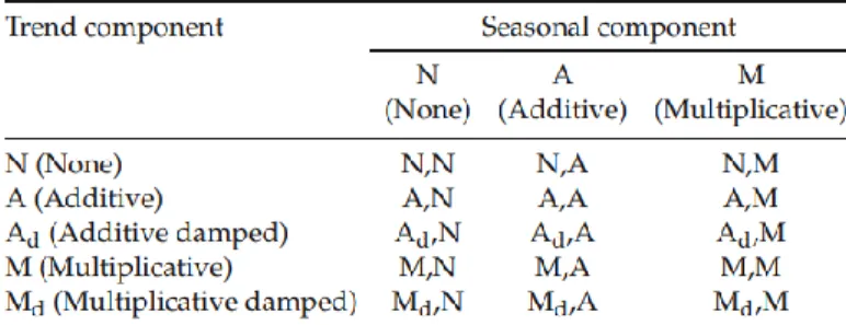
Hyndman et al (2002), Hyndman and Khandakar (2008) and Hyndman et al (2008) propose 15 different com- binations between trend and seasonality components. The trend component can present five different possibilities: none, additive, additive damped, multiplicative, and multiplicative damped. The trend component is a combination between the level (/!) and growth (b) parameter. Consider Th the forecast trend over the next h periods, and φ is a damping parameter (0 < φ < 1). So if there is no trend component, Th = /!. If the trend component is additive, Th = /! + bh. If the trend component is additive damped, Th = /! +
(
φ + φ2 + · · · + φh) b. If the trend component is the end of the series is unlikely to continue, the damped trend seems to be a reasonable option.
After we present the types of trend component, the next step is to detail the types of seasonal component. The seasonal component can be none, additive or multiplicative. Also the error component can be additive or multiplicative, but this distinction is not relevant to make point forecast (Hyndman et al, 2008).
So, we consider the combination of five types of trend component and three types of seasonal component which leads to a total of 15 types of exponential smoothing methods that we consider in this paper, following Hyndman and Khandakar (2008). We present these 15 possibilities in the Table 1, in which the first entry refers to the trend
n k k
10
m
component and the second to the seasonal component. Some of these exponential smoothing methods are known by other names. For example, cell N, N represents the simple exponential smoothing method, cell A, N refers to the Holt’s linear method, and cell Ad, N is associated with the damped trend method. The cell A, A describes the additive Holt-Winter’s method, the cell A, M refers to the multiplicative Holt-Winter’s method.
Table 1: The different combinations of exponential smoothing methods
For example, consider the Holt’s linear method (cell A, N ) that can be described as
/!t = αyt + (1 − α) (/!t−1 + bt−1) (20) bt = β∗ (/!t − /!t−1) + (1 − β∗) bt−1 (21)
yˆt+h|t = /!t + bth (22)
where equation (20) shows the model to the level of the series at time t /!t in this case. The equation (21) describes the growth rate (slope estimate) of the series at time t bt. bt is a weighted average of the estimate of growth obtained by the difference between successive levels and the previous growth bt−1. Finally, the equation (22) presents the prediction for the variable y h periods ahead using information available at time t. This equation describes that the forecast for the variable h periods ahead is given by the level in the current time /!t adding the growth bt for the h periods. α is the smoothing parameter for the level with 0 < α < 1, and β∗ is the smoothing parameter for the trend with 0 < β∗ < 1.
Now we consider a model with the seasonality component. When seasonal variations are constant throughout the series, the additive method for the seasonal component is preferred. When seasonal variations change proportionally to the level of the series, the multiplicative method for the seasonal component is preferred. Consider for example the Holt-Winters method of additive trend with additive seasonal component (cell A, A), the equations of this method are given by
/!t = α (yt − st−m) + (1 − α) (/!t−1 + bt−1) (23) bt = β∗ (/!t − /!t−1) + (1 − β∗) bt−1 (24) st = γ (yt − /!t−1 − bt−1) + (1 − γ) st−m (25)
yˆt+h|t = /!t + bth + st−m+h+ (26)
The equations (23), (24), (25), and (26) describe, respectively, the level /!t, the growth rate bt, the seasonality st, and the forecast h periods ahead of the series yˆt+h|t. m is the length of seasonality (e.g., number of months or
11 m
( )
quarters in a year), and h+ = [(h − 1) mod m] + 1. The parameters of the Holt-Winters method (α, β∗, γ) are
restricted to lie between 0 and 1.
Table 2 presents the equations for the level, growth, seasonality, and forecast of the series for h periods ahead for the 15 cases considered. Some values for exponential smoothing parameters lead to interesting specific cases. Some examples are: the level remains constant over time if α = 0, the slope is constant over time if β∗ = 0, and the seasonal behavior is the same over time if γ = 0. Finally, the methods A and M for the trend component are particular cases of Ad and Md with φ = 1.
Table 2: The equations for the level, growth, seasonality, and forecast of the series for h periods ahead for the 15 cases considered
In the sequence we present the state space models that underlie exponential smoothing methods. Each of the 15 models considered consist of a measurement equation that describes the data, and state equations that represent how the unobserved components (level, trend, seasonal) modify over time. The measurement equation together with the state equations are known by state space models.
Hyndman et al (2002) propose to differentiate the behavior of the model with additive errors in relation to the multiplicative errors. If the estimated parameters are the same, the point forecast is not affected if the error is multiplicative or additive, only the prediction interval. When considering the behavior of the error, Hyndman et al (2002) have the triplet (E, T, S) that refers to the three components: error, trend, and seasonality. The model ETS(A, A, N ) means that the errors and the trend are additive and that there is no seasonality for example.
If we return to the Holt’s linear method presented by equations (20), (21), and (22) with additive errors for example, we have ETS(A, A, N ). Assuming that error εt = yt−/!t−1−bt−1 N 0, σ2 and independently distributed, we
can write the error correction equations as
yt = /!t−1 + bt−1 + εt (27)
/!t = /!t−1 + bt−1 + αεt (28)
12
where β = αβ∗. Equation (27) refers to the measurement equation and equations (28) and (29) describe the state equations for the level and growth respectively. Similarly, all 15 exponential smoothing methods presented in the table 2 can be rewritten in the form of state space model with additive or multiplicative errors, see Hyndman et al (2008) for example.
Basically, the estimation procedure is based on estimating the smoothing parameters α, β, γ, φ and the initial state variables /!0, b0, s0, s−1,..., s−m+1 maximizing the likelihood function. The algorithm proposed by Hyndman et al.
(2002) also determines which of the 15 ETS models is most appropriate by selecting the model based on the information criterion. The information criterion used to select the most appropriate model are Akaike information criterion (AIC), AIC corrected for small sample bias (AICc), and BIC, according to Hyndman et al (2008).
3.5 Autometrics algorithm
We use the Autometrics algorithm (Doornik and Hendry, 2007, 2009, Doornik, 2009) to address potential instability points and structural changes and we select the lags of the dependent variable that are relevant. The algorithm is based on the approach called the London School of Economics of the general model to the particular. From a general unrestricted model, the algorithm attempts to reduce the unrestricted model through combinations between variables of the general model to evaluate the relevance of the variables to eliminate those irrelevant variables (variables with coefficients that are statistically insignificant). At each step in the attempt to reduce the model, the algorithm performs specification error tests in order to verify the congruence of the models after the eliminations. The purpose of this procedure is to determine the comprehensive and parsimonious model that is a good representation of the local data generating process. According to Hendry and Nielsen (2007), a model is congruent when it satisfies specification error tests for (i) heteroscedasticity, autocorrelation and non-normality, (ii) failure of the weak exogeneity hypothesis, (iii) constant parameters over time. The algorithm allows the number of variables to be greater than the number of observations and it deals with the perfect collinearity generated by the saturation dummy variables that we mention below.
We adopt the Autometrics algorithm with a significance level of 1% and 0.1% using the block method with the inclusion of impulse indicator saturation (IIS) and step indicator saturation (SIS) variables. We include all these variables at each point in time in the regression to analyze whether they are relevant through Autometrics algorithm. That is, if we have a regression with 100 observations in time, the algorithm analyzes the relevance of 100 possibilities for the dummy variable IIS for example. IIS is a dummy variable that is one only at a given point in time and zero otherwise. SIS is a variable equal to one from the beginning of the sample to the specific point in time and zero thereafter. The dummy variable SIS deals with the presence of structural breaks.
The Autometrics algorithm starts from a general model with up to 15 lags of the dependent variable for Brazilian industrial production with the following equation
15 T 11
yt =ρi yt−i +(αlIISl + γlSISl) +θsSes + εt
where SISl is a step dummy variable equal to one until t = l and zero otherwise, IISl is an impulse variable equal to one only at t = l and zero otherwise. Ses are the monthly dummy variables for each month s. εt is the error term.
4 Data and Empirical Strategy
Our data is the Brazilian industrial production index at general level and your disagreggation by sectors. The data source is the Monthly Industrial Survey of Physical Production (PIM-PF) of the Brazilian Institute of Geogra-
13
t+h|t −t+h −t+h
phy and Statistics (IBGE). We use monthly data from January 2002 to August 2017 without seasonal adjustment. We consider the first difference of data to have stationary series, with exception of the UC-SV and ETS models.
We forecast the general industry in a model only with the lags of this series and we compare this with the forecast for each sector and we aggregate according to their weight to obtain the general industry forecast. Thus we use the disaggregated data for the extractive industry and the 25 sectors of the manufacturing industry. However, two sectors printing and reproduction of recordings; and maintenance, repair and installation of machines and
equipment only present data from January 2012 and therefore we do not include these sectors in the estimates.2
Thus, our disaggregated sample includes the category of extractive industries and 23 sectors of the manufacturing industry. Next we detail the empirical strategy and how we compare the predictions obtained.
4.1 Empirical Strategy and Forecast Comparison
We consider the model up to 15 lags of the dependent variable. Thus, we use a rolling window of 100 fixed observations for each estimation for a forecast horizon of 1 to 12 months ahead. With this window size, we estimate 61 samples for general industry forecast series as for each of the sectors. We reestimate the model using LASSO-type methods, Autometrics algorithm, ETS and naive models for the rolling windows. Thus, we allow a re-specification of the best model according to each methodology for each window. We forecast the production of each sector and we use the weight of each sector to obtain the forecast for the general industry from its components. The forecast window for analysis ranges from September 2011 to August 2017.
We compare our forecasts with the estimates of three naive models. The first is the autoregressive model of the first order, the second is the time-varying parameters autoregressive model of the first order, and the third is the UC with SV. We estimate all models with the data for the general industry (aggregate forecast) and the forecast for the general industry from the disaggregated data (disaggregated forecast). Thus, we have two naive predictions from the AR (1) model (aggregate and disaggregated), two naive predictions from the time varying AR(1) (aggregate and disaggregated), and two naive predictions from UC with SV (aggregate and disaggregated). The naive model serves as reference or benchmark for the other forecasts. The performance analysis for the forecast from the models will be through the mean square error (MSE), the Diebold and Mariano (1995) test and Model Confidence Set of Hansen et al (2011) to determine if there is a model with more accurate prediction for the Brazilian index of general industrial production for the period considered. Next we present the test of Diebold and Mariano (1995).
4.1.1 Diebold and Mariano test
The MSE is the difference between the actual value of the data and the estimated value squared. The MSE is an average of this squared difference for the sample forecasts.
The Diebold and Mariano (1995) test presents if there is any model that has a statistically more accurate prediction for the Brazilian general industrial production for the considered period. Consider a loss function g based on forecasting errors, in which we consider a quadratic loss function. Assuming two models (1 and 2), in
which the forecasting errors εˆ for h period ahead are given by εˆ1
t+h|t = y yˆ 1 t+h|t and εˆ 2 t+h|t = y yˆ 2 , t+h|t where yˆ2
t+h|t is the forecast from model 2 for h periods ahead for example. The Diebold and Mariano (1995) test is
based on the difference between the forecasting error of the models.
The null hypothesis of the test is that there is equality of forecasting performance between the two models, that is, the models have statistically equal deviations. On the other hand, the alternative hypothesis (one-sided test) defines that the model used as a reference leads to more accurate forecasts than the other. We need to define the forecasts of one of the models as a benchmark for the test, which we will do based on the results from the MSE. The Diebold and Mariano (1995) test is given by:
14 t=1 t+h|t − ¯ vˆar( d ) T0 t=t0 t+h|t t+h|t S = d¯ A var (d¯) (30) where d¯ = 1 T dt, dt = g εˆ1
− g εˆ2 , and A var (d¯) is an estimate of the asymptotic variance (large
samples) of d¯ for the sample selected. Thus, the S statistic follows a Student t-distribution (Diebold, Mariano, 1995). We consider the quadratic loss function for the test performed in the present work.
4.1.2 Model Confidence Set
Hansen et al (2011) propose the Model Confidence Set (MCS). The interpretation of MCS is similar to a confidence interval. The advantage of this procedure is that it does not require imposing a benchmark. This
procedure allows to obtain a set of models that contain the best model with a certain level of confidence. MCS1−α considers the best model with 100(1 − α)% confidence. The set contains more models if we decrease α.
MCS uses a loss function to create the test statistics. We use squared errors as the loss function. The MCS procedure estimates p-values for all models from this statistics, in which the variance is calculated by the bootstrap estimation. The null hypothesis of MCS is the equal predictive ability between the models of the set.
Consider the loss statistics d¯ij = n−1 n dij,t where dij,t = g εˆi g εˆjt+h|t , g as a quadratic function and we have the sample size n for the prediction errors. d¯ij is the relative loss between the ith and jth models and
d¯i = m−1 j∈M dij, where d¯i is the loss of the ith model relative to the average across models in M.
We obtain the set of models until the null hypothesis is no longer rejected for α that we establish. Hansen et al (2011) present two different statistics: Tmax,M and TR,M . We consider the first statistic because it is simple and easy to compute. The second statistic compares all models two by two to get the set, but the computational process is more intense. We construct the statistics
d¯i ti =
i
Note that vˆar(d¯i) is the bootstrapped estimate of var(d¯i). Tmax,M = maxi∈M ti, where ti is the statistics about the sample loss between ith and across models in M . The asymptotic distribution of this statistic is nonstandard and Hansen et al (2011) propose to use bootstrap methods.
Then, the algorithm is a sequential procedure and it starts by stating that the set of models is the total of models considered in the work, that is, M = M 0 in the first step. The second step is to test the null hypothesis at level α. The
third step is if the null hypothesis is accepted, the final set is M = M 0; otherwise we eliminate the model with the
lowest p-value from M and we repeat the procedure considering M = M 1, where M 1 is M 0 without the worst model
by the p-value.
5 Results
This section presents the forecasts of 1 to 12 months ahead for the naive models - AR(1), AR(1) with time- varying parameters, UC with SV - besides the lag selection from the LASSO and its two variants (adaLASSO and WLadaLASSO), exponential smoothing ETS and Autometrics with and without the inclusion of IIS and SIS variables to forecast the general industry from aggregated and disaggregated data. We have four types of forecasting models with Autometrics. The first is ’without outlier’ which does not consider any type of outlier in the general model. The second is ’IIS’ that allows only the dummy variables to control for outlier. The third is the ’SIS’ that allows only the step dummy variables. Finally, ’IIS and SIS’ allows all possible break and outlier variables. We compare the results in three parts, based on the MSE, the Diebold and Mariano (1995) test and the MCS to obtain the model with the most accurate forecast.
15
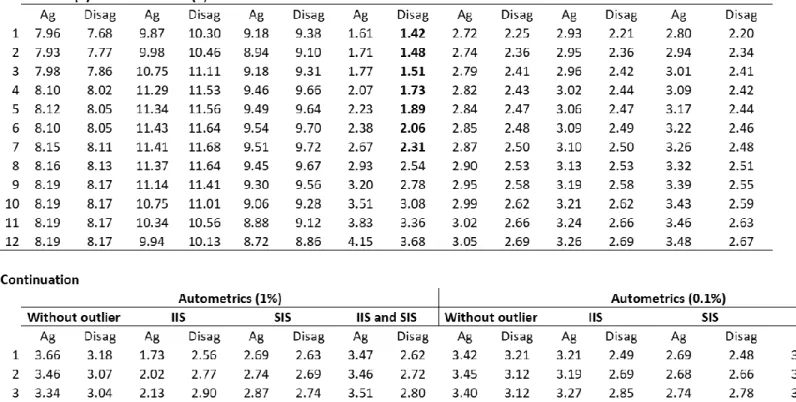
Table 3 presents the MSE of 1 to 12 months ahead for the different models. We multiply the MSE value by 104 to
improve the visualization of the results presented in the table 3. We also put in bold and red the lowest MSE per forecast horizon to make it easier to see the table 3. In general, we can analyze that the MSE is smaller for the disaggregated models in relation to the aggregates independent of the forecast horizon, with the exception of AR (1) with time-varying parameters and UC with SV. The model with the lowest MSE for the forecast of one to seven months ahead is disaggregated ETS. Increasing the forecast time horizon mainly from one to three periods ahead does not greatly affect the MSE of the disaggregated ETS. The Autometrics algorithm presents lower MSE for the time horizon of eight to twelve months. The Autometrics algorithm with SIS variables and a significance level of 0.1% for disaggregated data presents lower MSE for the time horizon of 10 to 12 months ahead. The Autometrics algorithm with IIS dummy variables and with significance level of 1% using aggregate data has the lower MSE only for seven months forward. This is the only model with aggregate data that has lower MSE and it is only in one step forward. Also the Autometrics algorithm with SIS variables and significance level of 1% has the lower MSE for eight months forward. The disaggregated ETS has an increase in MSE for the steps forward while the Autometrics algorithm has not a growth in MSE for larger horizons in general.
The difference in MSE between the LASSO models and variants is small mainly using disaggregated data, in which the disaggregated WLadaLASSO performs better than the other disaggregated LASSO-type methods for the different forecast horizons. However, when we estimate the aggregate model, the LASSO model presents better prediction performance in relation to its variants. An interesting point would be to try to find out why WLadaLASSO does not perform better than its variants for aggregate data or why there is this difference of performance between aggregated and disaggregated data. Konzen and Ziegelmann (2016) point out that WLadaLASSO would perform better than LASSO and adaLASSO when the sample is small and the greater the number of lags used but we are not varying these two points.
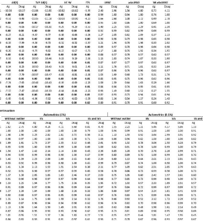
The MSE difference does not allow to state if the disaggregated ETS has higher accuracy of the forecast statistically in relation to other methods. Therefore, we analyze the results of the Diebold and Mariano (1995) test. In order to perform the test, we establish the disaggregated ETS as the benchmark model because it has lower MSE of 1 to 7 months ahead compared to the rest of the models, indicating forecast power gains. We compare the forecast errors of all models with those of the benchmark, having as null hypothesis the equality of predictive power. Under the null hypothesis, the disaggregated ETS predicts as well as the analyzed model. The alternative hypothesis indicates that the prediction of the disaggregated ETS is statistically better.
Table 4 presents the Diebold and Mariano (1995) statistic and the associated p-value (below the test statistic) for each of the models in relation to the benchmark. We present in bold and red the p-value when we reject the null hypothesis to facilitate the visualization and interpretation of the table 4. From the results of Diebold and Mariano (1995) test, we can consider that the disaggregated ETS presents better statistical performance for forecast in relation to the naive models (AR(1), AR(1) with time-varying parameters, UC with SV) considering aggregate or disaggregated data and aggregate ETS. However, the disaggregated ETS model does not present better accuracy in relation to the LASSO models and their variants or the Autometrics algorithm models with or without dummy variables, regardless of being aggregated or disaggregated.
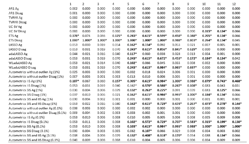
But only the MSE is not enough to say whether the forecasting difference between the models is statistically significant. We perform the MCS procedure to obtain which models we can consider as the best. Table 5 presents p-values from the MCS and those models in the set of “best” models with 90% of probability are indicated with one asterisk (and are in bold and in red). We select only ETS models (with aggregated and disaggregated data) and the Autometrics algorithm with IIS dummy variables with aggregated data with 1% of significance level for one
Table 3: MSE results for forecasting from 1 to 12 months ahead for different models
Table 4: Diebold and Mariano (1995) test results from 1 to 12 months ahead for different models
and four steps forward. Only the disaggregated ETS remains in the MCS for forecast horizons of 2 and 3 periods forward. The best model to forecast 5 to 11 months ahead is composed mostly of models with disaggregated data. The best model has the ETS models, Autometrics, LASSO, adaLASSO and WLadaLASSO.3 The best model to forecast
12 months ahead includes only the models selected by the Autometrics algorithm. The two best models out of the four in the MCS for 12 periods forward are the aggregates with Auometrics.
Conclusions
The present work seeks to analyze two points about forecasting Brazilian industrial production. The first is to compare different univariate models for selection of lags like LASSO and two variants, exponential smoothing models and Autometrics algorithm. Among these models, which type of model has the best forecast for the Brazilian industrial production. The second point is to consider whether the disaggregated data contribute to predict the aggregate level of industrial production. Basically our result points to a better performance of models that use disaggregated data in relation to aggregated data. The exponential smoothing model with disaggregated data performs better in the forecast from 1 to 7 months ahead. The Autometrics algorithm with impulse and structural break variables offers better forecasting performance from 8 to 12 months ahead. The model selected by the Autometrics algorithm generates forecasts with the lowest MSE for 10 to 12 steps forward specifying a lower significance level (0.1%) and including structural break variables with disaggregated data. The difference in performance between the LASSO and its variants (adaLASSO, WLadaLASSO) is small when we consider the disaggregated data.
Epprechat et al (2019) obtain a different result that adaLASSO and Autometrics have similar forecasting per- formance with small values of relevant variables and when the candidate variables are lower than the number of observations. The Autometrics algorithm only performs better when they have a large value of relevant variables because of the bias from the penalization term in adaLASSO, according to the authors. In our case, the Autometrics algorithm always has a better performance than the LASSO type penalties.
This is an ongoing research. The next steps are to contemplate two additional models for forecast, which is the lag selection with dynamic model averaging/selection framework of Koop and Korobilis (2012) and Raftery et al (2010) and bagged ETS of Bergmeir, Hyndman and Benï¿œtez (2016).
References
Barhoumi, K., Darnï¿œ, O., and Ferrara, L. (2010), “Are disaggregate data useful for factor analysis in forecasting French GDP”, Journal of Forecasting, 29, 132-144.
Barnett, A., Mumtaz, H., and Theodoridis, K. (2014), “Forecasting UK GDP growth and inflation under struc- tural change. A comparison of models with time-varying parameters”, International Journal of Forecasting, 30, 129-143.
Carlos, T., and Marï¿œal, E. (2016), “Forecasting Brazilian inflation by its aggregate and disaggregated data: a test of predictive power by forecast horizon”, Applied Economics, 48, 4846-4860.
Carter, C., and Kohn, P. (2004), “On Gibbs sampling for state space models”, Biometrika, 81, 541–53.
Chib, S. (1995), “Marginal likelihood from the Gibbs output”, Journal of the American Statistical Association, 90, 1313–21.
Chib, S., and Jeliazkov, I. (2001), “Marginal likelihood from the Metropolis-Hastings output”, Journal of the American Statistical Association, 96, 270–81.
3Only for two forecast horizons we have the UC-SV model in the best model.
Table 5: Model Confidence set p-values from 1 to 12 months ahead for different models
19
Crone, S., and Kourentzes, N. (2010), “Feature selection for time series prediction – a combined filter and wrapper approach for neural networks”, Neurocomputing, 73, 1923-1936.
Duarte, C., and Rua, A. (2007), “Forecasting through a Bottom-up approach: how bottom is bottom?”, Economic Modelling, 24, 941-953.
Epprecht, C., Guegan, D., Veiga, A., Rosa, J. (2019), “Variable selection and forecasting via automated methods for linear models: LASSO/adaLASSO and Autometrics”, Communications in Statistics - Simulation and Compu- tation, forthcoming.
Espasa, A., Senra, E., and Albacete, R. (2002), “Forecasting inflation in the European Monetary Union: a disaggregated approach by countries and by sectors”, European Journal of Finance, 8, 402-421.
Giacomini, R., and Granger, C. W. J. (2004), “Aggregation of space-time processes”, Journal of Econometrics, 118, 7-26.
Granger, C. W. J. (1987), “Implications of aggregation with common factors”, Econometric Theory, 3, 208-222. Hansen, P., Lunde, A., and Nason, J. (2011), “The Model Confidence Set”, Econometrica, 79(2), 453-497. Harvey, D., S. Leybourne, and P. Newbold. (1997), “Testing de equality of prediction mean squared errors”, International Journal of Forcasting, 13, 281–291.
Hendry, D. F., and Hubrich, K. (2011), “Combining disaggregate forecasts or combining disaggregate information to forecast an aggregate”, Journal of Business and Economic Statistics, 29, 216-227.
Hyndman, R., Koehler, A., Snyder, R., and Grose, S. (2002), “A State Space Framework for Automatic Fore - casting Using Exponential Smoothing Methods”, International Journal of Forecasting, 18, 439-454.
Hyndman, R., Koehler, A., Ord, J., and Snyder, R. (2005), “Prediction Intervals for Exponential Smoothing Using Two New Classes of State Space Models”, Journal of Forecasting, 24, 17-37.
Hyndman, R., and Khandakar, Y. (2008), “Automatic Time Series Forecasting: the forecast package for R”, Journal of Statistical Software, 27, 1-22.
Hyndman, R., Koehler, A., Ord, J., and Snyder, R. (2008), Forecasting with exponential smoothing, Springer, Berlin.
Hubrich, K. (2005), “Forecasting euro area inflation: Does aggregating forecasts by HICP component improve forecast accuracy?”, International Journal of Forecasting, 21, 119-136.
Jacquier, E, Polson, N, and Rossi, P (2004), “Bayesian analysis of stochastic volatility models”, Journal of Business and Economic Statistics, 12, 371–418.
Kapetanios, G., Marcellino, M., and Venditti, F. (2017), “Large time-varying parameter VARs: a non-parametric approach”, Bank of Italy working paper no. 1122.
Koch, A, Terï¿œsvirta, T. (2014), “Forecasting performances of three automated modelling techniques during the economic crisis 2007–2009”, International Journal of Forecasting, 30, 616-631.
Koop, G., and Korobilis, D. (2012), “Forecasting Inflation Using Dynamic Model Averaging”, International Economic Review, 53(3), 867–886.
Kourentzes, N., Barrow, D., and Crone, S. (2014), “Neural network ensembles operators for time series forecast- ing”, Expert Systems with Applications, 41, 4235-4244.
Kroese, D., and Chan, J. (2014), Statistical Modeling and Computation, Springer, Berlin.
Lï¿œtkepohl, H. (1984), “Linear transformation of vector ARMA processes”, Journal of Econometrics, 26, 283- 293.
Lï¿œtkepohl, H. (1987), Forecasting Aggregated Vector ARMA Processes, Springer-Verlag, Berlin.
Marcellino, M., Stock, J. H., and Watson, M. W. (2003), “Macroeconomic forecasting in the Euro area: Country specific versus area-wide information”, European Economic Review, 47, 1-18.
Ord, J., Koehler, A., and Snyder, R. (1997), “Estimation and Prediction for a Class of Dynamic Nonlinear Statistical Models”, Journal of the American Statistical Association, 92, 1621-1629.
20
Raftery, A., Karny, M., and Ettler, P. (2010), “Online Prediction Under Model Uncertainty via Dynamic Model Averaging: Application to a Cold Rolling Mill”, Technometrics, 52(1), 52–66.
Stock, J., and Watson, M. (2007), “Why has U.S. inflation become harder to forecast?”, Journal of Money, Credit and Banking, 39, 3-33.
Tibshirani R. (1996), “Regression shrinkage and selection via the lasso”, Journal of the Royal Statistical Society, Series B, 58, 267–288.
Weber, E. and Zika, G. (2016), “Labour market forecasting in Germany: is disaggregation useful?”, Applied Economics, 48, 2183-2198.
Zhao, P., and Yu, B. (2006), “On model selection consistency of Lasso”, Journal of Machine learning research, 7, 2541-2563.