INTERNATIONAL MICROSIMULATION ASSOCIATION
Cash Transfer Policies, Taxation and the Fall in Inequality in Brazil An Integrated Microsimulation-CGE Analysis
Samir Cury
Fundação Getúlio Vargas (EAESP/FGV), São Paulo, Brazil Departamento de Planejamento e Análise Econômica (PAE)
Av. 9 de Julho, 2029, Bela Vista, PO code: 01313-90. São Paulo – SP, Brazil e-mail: [email protected]
Euclides Pedrozo
Fundação Getulio Vargas (EESP/FGV) and Universidade Paulista, São Paulo, Brazil
Rua Afonso Celso, 171, Ap. 163A – Vila Mariana, PO code: 04119-000, São Paulo - SP, Brazil e-mail: [email protected]
Allexandro Mori Coelho
Centro Universitário Álvares Penteado (FECAP), São Paulo, Brazil.
Avenida Liberdade, 532 - Liberdade, ZIP: 01502-001, São Paulo – SP, Brazil e-mail: [email protected]
ABSTRACT: Persistent and very high-income inequality is a well-known feature of the Brazilian
economy. However, from 2001 to 2014, the Gini index registered an unprecedented fall of 13.5% percent, combined with significant poverty reduction. Previous studies using partial equilibrium analysis have pointed out the important role of federal government transfer programs in this inequality reduction, particularly in the first period (2001-2005) when the new trend started. The aim of this research is to evaluate the efficiency of the two most important cash transfer programs, “Bolsa Família (PBF)” and “Benefício de Prestação Continuada (BPC)”, in achieving their purpose of alleviating poverty and reducing inequality in Brazil’s income distribution. The simulation results, using an integrated modeling approach, confirm the importance of these programs in reducing inequality from 2003 to 2005. However, the effect on poverty alleviation was not strong. Finally, the methodological approach reveals some important mechanisms that were not present in
previous analyses, such as the role of the tax structure that finances these policies.
KEYWORDS: poverty, inequality, cash transfer program, fiscal policy, computable general
equilibrium model, microsimulation model, Brazil.
1. INTRODUCTION
It is widely known that Brazil has one of the most unequal income distributions in the world, with a Gini index around 0.60 until the beginning of this century.1 This high income inequality has been one of the main causes of the country’s equally high levels of poverty, despite often strong economic growth.
However, from 2001 to 2014, there was an unprecedented and continuous fall in income inequality, with the Gini index declining 13.5% from 0.594 to 0.5132. This has coincided with a significant reduction of poverty. Between 2001 and 2014, the percentage of poor declined from 38.7% to 15.3%, while the percentage of extremely poor declined from 17.4% to 4.6%.3 These evolutions coincided with the introduction and expansion of targeted income transfer programs as part of a national poverty alleviation strategy.
There are many kinds of income transfer programs in Brazil, such as Programa Bolsa Família (PBF),
Benefício de Prestação Continuada (BPC)4 and several retirement benefits and pensions. This research analyzes the first two programs (PBF and BPC) because they are the main cash transfer programs specifically designed as social policies with the purpose of poverty (and inequality) reduction.
PBF was created in October 2003 and is presently the federal government’s main cash transfer
program. It is a cash transfer program with conditions such as 85% school attendance for children in schooling age, vaccination for children under six years old, and regular visits to a health center for both pregnant and breastfeeding women. In 2005, PBF had a total of 10.6 million beneficiary households and R$6.9 billion worth of transfers (equivalent to 0.3% of GDP in 2005).
BPC is a social assistance benefit since 1996. It aims to aid the elderly who are not included in the
public social security system and the disabled who cannot support themselves despite their households’ financial care. Both beneficiary groups comprise 2.8 million beneficiaries, with a budget of R$9.7 billion (or 0.4% of GDP) for BPC in 2005. The benefit consists of a cash transfer amounting to one minimum wage (R$300 in 2005) where the beneficiary’s family per capita income must be less than a quarter of the minimum wage.
These programs aim to reduce poverty and income inequality, hence the need for evaluations of their effects. The most common approach is partial equilibrium and decomposition analysis. Hoffmann (2006b) points out that 31% of the decline in Brazil’s inequality – 87% in the country’s Northeast region – from 2002 to 2004 were due to the above mentioned programs. Barros et al. (2007c) estimated that PBF and BPC induced, respectively, around 11.8% and 11.1% of the fall in
income inequality from 2001 to 2005. According to IPEA (2012), during the period from 2001 to 2011, these two programs contributed to reduce inequality by 17% (and up to 24% between 2003 and 2005).
The contribution of PBF and BPC is more impressive if one takes into account the limited budget of these public policies. In 2013, the total budget of the public social security system represented 10.9% of GDP (6.8% for the general system – INSS, and 4.1% for former public workers) while
PBF and BPC represented only 0.5% and 0.65%, approximately.5
However, these partial equilibrium or decomposition approaches do not take into account systemic (general equilibrium) effects induced by these programs on the economy, as well as the feedback impacts to household income and consumer prices. When poor households receive transfers, they tend to consume more, which stimulates production and employment, and so on through a multiplier effect. These demand effects are enhanced when we take into account differences in the expenditure patterns of Brazilian households by income level. Among poor urban Brazilian households, food expenditure is 40% of total consumption, compared to only 12% for the richest households (Cury et al., 2006).
In addition, the relevance of the general equilibrium effects is justified by the size and evolution of the transfer programs. Almost 14 million households (around 20% of all households) are PBF beneficiaries, covering more than 50 million individuals (around 25% of the population). In 2014, the total value of cash transfers was R$27.2 billion, representing more than 0.5% of the Brazilian GDP.
In addition, we may expect that program effects are sensitive to the mechanism chosen to finance this specific public expenditure, which generate direct and general equilibrium effects of their own. Also, during 2003-2005 some important changes were introduced in the fiscal system. For example, in the social security budget, the sharpest revenue increase came from PIS-COFINS taxes (a rise of 30% in their GDP ratio), which in 2003-2004 started to levy imports.
Additionally, cash transfers may cause some beneficiaries to reduce labor supply. This may counteract some of the benefits of these programs. Recently, several studies aimed to estimate the effects of the PBF and other conditional cash transfer programs on adult labor supply in Brazil (e.g., Soares et al., 2007; Ferro and Nicollela, 2007; Teixeira, 2008; Covre et al., 2008; and Foguel and Barros, 2008). These studies use different empirical strategies to compare beneficiaries against comparable non-beneficiaries.
There is some evidence that PBF can reduce labor market participation mainly among beneficiary mothers. For example, Tavares (2008) found evidence of an adverse effect of PBF on beneficiary mothers’ willingness to participate in the labor market due, mainly, to the program's conditionalities (education and health of children). On the other hand, Firpo et al. (2014) find evidence that some individuals (particularly women) deliberately reduce their labor income in order to qualify for the
PBF. Similarly, Santos (2013) shows that the PBF has encouraged adult beneficiaries to offer
informal labor. In both cases, the purpose of the beneficiary is hiding the real family income to continue receiving the cash grant.
Proving that a specific methodology is unequivocally superior to others is not an easy task. However, according to Cockburn et al. (2015), the analysis of the impacts of large-scale policies on income distribution requires the usage of tool that integrates microsimulation (MS) techniques and a computable general equilibrium (CGE) model. Given the systemic consequences of the PBF and
BPC programs and their financing mechanisms on the overall economy, we adopt a CGE model
integrated with a Microsimulation model (CGE-MS model) approach to evaluate the impacts of these programs on poverty and inequality in Brazil.
This paper is organized into five sections, including this introduction. The next section describes the methodology: the CGE model, the MS model, and their integration. The research questions, simulation scenarios and results are presented in section 3. The last section presents the conclusion and the final remarks.6
2. METHODOLOGY
This study applies a CGE-MS combined iterative approach, where the starting model (i.e. where the first shock is applied) is the MS model. For this reason, this kind of approach is referred to as bottom-up/top-down in the literature (see Cockburn et al., 2015, for a discussion of the various CGE-MS approaches).
2.1. The CGE Model
This section briefly describes some key characteristics of the CGE model. Further details on this model can be found in Cury et al. (2010, Appendix A.2).7 The CGE model distinguishes 42 domestic sectors, 8 household types,8 the Government, and the external sector. The model assumes that the Brazilian economy is an international price taker but that the changes of its export prices can affect the external demand for Brazilian goods through an export demand equation. Production
is a function of 7 types of labor,9 capital and intermediate inputs and sold as imperfect substitutes in the domestic and international markets.10 Households and firms demand domestic and imported goods according to the Armington (1969) hypothesis.
In terms of closure, the nominal exchange rate is exogenous, while the price index is endogenous. Foreign savings is also exogenous, which implies a fixed balance of trade. Government spending is fixed exogenously, but the total public deficit is endogenous. Investment is determined by total savings where the marginal propensity to save is fixed.
2.2. The Microsimulation Model (MS)
The database for the microsimulations is the National Survey by Household Sampling 2003 (PNAD 2003). It contains a nationally representative sample of almost 384,834 individuals distributed in 117,010 households.11 As it does not contain information about household expenditures, the MS model focuses on individual labor supply.
Each working-age individual (over 10 years old) was classified according to the seven labor categories in the CGE model. Formal and informal workers are assumed to have flexible wage. However, as public servants in Brazil benefit from a job stability clause, it is assumed that their employment levels are fixed.12 The sample includes 106,590 working-age individuals, representing 48,742,853 individuals in the total population.
The MS model is based on Savard (2003). The main adaptation for this model is the use of a segmented labor market.13 For the unemployed, the reservation wage of each individual determines the choice to supply (or not) labor in the market.
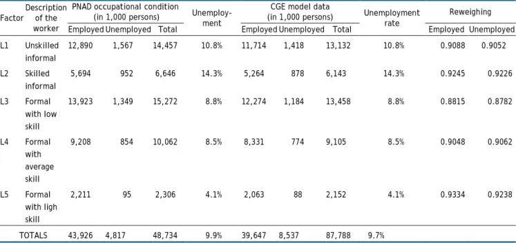
One of the main difficulties in making CGE-MS integration work is convergence. For this convergence to be successful the two databases must have the same values. Thus, the individual weights were multiplied by a factor (reweighting) so that the PNAD 2003 database reflects the CGE model data. Table 1 presents the results of this reweighting for employed and unemployed people.
Table 1 Employed and unemployed reweighing for L1 to L5 work factors
Factor
Description of the worker
PNAD occupational condition
(in 1,000 persons) Unemploy-ment
CGE model data
(in 1,000 persons) Unemployment rate
Reweighing Employed Unemployed Total Employed Unemployed Total Employed Unemployed L1 Unskilled informal 12,890 1,567 14,457 10.8% 11,714 1,418 13,132 10.8% 0.9088 0.9052 L2 Skilled informal 5,694 952 6,646 14.3% 5,264 878 6,143 14.3% 0.9245 0.9226 L3 Formal with low skill 13,923 1,349 15,272 8.8% 12,274 1,184 13,458 8.8% 0.8815 0.8782 L4 Formal with average skill 9,208 854 10,062 8.5% 8,331 774 9,105 8.5% 0.9048 0.9062 L5 Formal with ligh skill 2,211 95 2,306 4.1% 2,063 88 2,152 4.1% 0.9334 0.9238 TOTALS 43,926 4,817 48,734 9.9% 39,647 8,537 87,788 9.7%
Source: PNAD 2003, CGE model data base.
A prior concern regarding the individuals’ reservation wage estimation is the issue related to labor supply identification. In principle, the expansion of income transfers exogenously affects the willingness to supply labor of various demographic groups in different ways. Thus, it is necessary to estimate an equation for individual labor supply, identified by the number of individual work hours, as a function of the individual wage-hour after changes in income transfers for each demographic group has been considered. It is also necessary to correct the potential auto-selection bias to labor supply participation. After applying this procedure, it is possible to properly identify the different reactions of the labor supply to exogenous changes in the size of transfers for individuals in each demographic group. Therefore, the estimation procedure can be described in two steps as follows:
Step 1
At this microsimulation stage, we are interested in the individual impact due an income transfers shock, especially for the demographic group of single mothers who are heads of household. This demographic group is the main beneficiary of the PBF and deserves special attention because it is the most sensitive to non-labor income from transfer programs, as found in our MS model results.
Our empirical strategy is based on a simpler version in which the worker makes an individual decision. Due to the identification problem of the non-linear budget constraint, we estimated a reduced-form hour equation as a function of the individual’s wage, the income from transfers
programs, other income, and a number of demographic controls. The “other income” variable combines all sources of non-labor income, following Blundell and McCurdy (1999). This last variable for married women, for example, is calculated by taking the husband’s actual earnings into account. On the other hand, we created another variable that represents the BPC and PBF programs in order to capture the effects of the income transfers on labor supply.14
The predicted working hours are obtained from the observed and non-observed individual and household characteristics and his own wage. Therefore, the worker i’s predicted hours of work (h ) is estimated by the semi-log specification according to Blundell and McCurdy (1999):ij
15
, 1,..., and 1,2,3 log log log w Q B Z u i n j hj i i i i i i i i i i (2.2.1)where , i ,i , i and i are the parameters to be estimated; i w is the hourly wage rate for i
individual i ; Q is the vector of the total household income net of the earnings (including income i
transfers) received by the individual i ; B is the vector of benefits received (PBF and BPC) by i
individual i in 2003; Z represents the individuals’ observable characteristics; i u is the random i
error term, which captures the non-observable characteristics that affect the individual labor supply; and j is the individual’s demographic group, 1 being for men, 2 for woman head of household with children, and 3 for other women (who are not heads of households). The value of
determines the substitution effect related to sensitivity of individual labor supply to changes in
wages. The values of and represent the income effect, that is, the impact of non-labor income on labor supply.
The Z vector of individual characteristics was composed of the following variables: i
a i educ ge ge famsize D
Z ,a ,a 2, ,
where educ denotes the number of years of schooling, age is a proxy to the level of experience; famsize is the family size in terms of number of individuals (excluding pensioners, domestic servants and their parents), D is a dummy for the area where the family’s domicile is located (0 for urban and a
1 for rural).
Individual working hours are observed only for those who are already employed. Thus, the sample of individuals that present strictly positive work hours is not random. However, it is possible that the choice to work is related to income-dependent variables, either from labor or non-labor (other
income sources). Therefore, the situation is typically one of endogenous selection, in which there is a decision to participate or not in the labor market and, given that the individual had decided to work, it is necessary to determine how many working hours he will offer. In order to control for potential selection bias, the procedure proposed by Heckman (1979) is applied, which consists of:
Si 1|z
i
YiZi
Pr(2.2.2)
where is a function of accumulated distribution, where S is a qualitative variable representing i
the occupational choice for an individual i: this variable will take the value 0, if the individual does not supply work, or 1, if otherwise. The variable is a vector of estimated parameters that i
determine the probability that the individual takes part in the labor market. Y is the vector i
representing the variables related to labor and non-labor incomes that affect the decision to supply labor by individual i. As before, Z are the individual characteristics that determine the probability i
of participating in the labor market.
The equations (2.2.1) and (2.2.2) are estimated by a two-stage method proposed by Heckman (1979). In this model, equation (2.2.2) corrects sample selection bias by non-observables. The selection variables used for identification are educ, age, age2 and famsize. To test and correct the sample
selection bias we estimate a probit model of labor market participation with these selection variables. These equations are run separately for three demographic groups: men, female household heads with children, and other women, to estimate the elasticity of labor supply. The inverse of Mills’ ratio z
is extracted from equation (2.2.2), which is applied to equation (2.2.1) to ensure that the parameters of these equations are consistently estimated.After estimating the coefficients in (2.2.1) and the inverse of Mills’ ratio, it is possible to estimate the adjusted working hours of each individual, h , based on observed and non-observed ij
characteristics. Adjusted working hours are then applied to the individual i’s observed wage, wˆ , i
which results in the adjusted individual i’s wage (w ).i 16
Step 2
The second part of the microsimulation process is the computation of the reservation wages and the new employment ratio. Individual labor supply is a function of individual market wage rates and non-labor income, among other variables. These wage rates can be observed for wage workers. For others there is an unobservable wage rate that an individual could potentially receive.
According to Heckman (1974) it is possible to express this reservation wage as a function of their individual characteristics as well as non-labor income and other constraints.
Following Savard (2003), the non-observed reservation wage is obtained from the observable and non-observable individual’s characteristics, as well as household characteristics. Due to the importance of evaluating the reservation wage before and after an income transfer shock, we include non-labor income in the structural reservation wage equation and identify the income transfer variable separately. Therefore, the worker i’s reservation log wage, w , is estimated by the i
equation:
Z u i n B Q wi i ilog i log i i i, 1,..., log (2.2.3)where , i , i and i are the parameters to be estimated. The observed wage, i wˆ , is the hourly i
wage adjusted by the procedure described in step 1;17 Q , i B and i Z are the same variables i
presented earlier.
Due to the impossibility of observing the wage offer to the sample’s unemployed individuals, we need to estimate a probit model that determines the probability of these individual taking part in the labor market. This probability,Si 1, is estimated by the function:
Si 1|z
i
YiZiDg
Pr (2.2.4)
where: is a function of accumulated distribution; is a vector of estimated parameters that i
determine the probability of the individual taking part in the labor market; as before, Z and i Y i
are, respectively, the individual characteristics and the work and non-work income that determine the probability of participating in the labor market; and D is a demographic dummy (0 for man, 1 g
for female household heads with children, 2 for other women).
As for equations (2.2.1) and (2.2.2), equations (2.2.3) and (2.2.4) are estimated by the Heckman two-stage method. This makes it possible to calculate the reservation wage of each individual, w ik
(k = 0,1) based on observed and non-observed characteristics. If the individual belongs to state 1
k , the reservation wage of worker i will be used in comparison with the observed wage, wi , to select among the potential employed or unemployed persons. If in state k 0, the reservation wage of this individual is obtained to construct a rank of potential newly employed persons.
If the estimated reservation wage (wij) is higher than the earned wage (w ) observed in the j
database, then this person is indicated as potentially unemployed; otherwise, he remains employed, i.e.: employed y potentiall is he , otherwise unemployed y potentiall is individual , if wi wik i
After making this comparison for each employed person, the model determines the Heckman pre-simulation occupational level by private labor type
HLsl by summing up the number of people
originally unemployed with the number of people that would be unemployed according to the Heckman criterion. It deserves mentioning that this occupational level is different from the original level in the database
Lsl , given that there are people in the database that work and earn wages
lower than their estimated reservation wages. This occurs because the latter wages are estimates of what these people could earn in the market according to their individual and household characteristics. Therefore, merely applying the Heckman procedure to the database changes the occupational level for each labor type.
As proposed by Savard (2003), the selection of individuals who should be unemployed starts with classifying workers according to their reservation wages. Those with the highest reservation wage will be the first to become unemployed if the real wage decreases. If there is a positive change in the real wages, the first to be employed will be those with the lowest reservation wage.18
Step 3
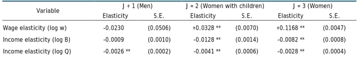
In this section we evaluate the relationship between the conditional cash transfer programs and individual work decisions through substitution and income effects. In table 2 we present the marginal effects in respect to hours of work, implied by the estimates from steps 1 and 2.
The wage compensated elasticity of labor supply reflects the strength of the substitution effect from the perspective of labor income. The wage elasticities are the coefficients reported by the variable logw in equation (2.2.1). For women without children (j = 3) this elasticity is positive and higher than for women who are household heads (j = 2), which is to be expected according to the results of many empirical studies. For men, the negative elasticity is not usual, but it is statistically non-significant.
income elasticities described by the variables logB (public transfer benefits) and logQ (all other non-labor income) in equation (2.2.1) are all negative, as expected. The highest sensibility is related to the group formed by female household heads with children, which is in line with the great majority of empirical work on this subject. Also, the results are consistent with standard theory and show that cash benefits may have participation effects on specific population groups.
Table 2: Elasticities - Marginal effects for grouping demographics
Variable J + 1 (Men) J = 2 (Women with children) J = 3 (Women) Elasticity S.E. Elasticity S.E. Elasticity S.E. Wage elasticity (log w) -0.0230 (0.0506) +0.0328 ** (0.0070) +0.1168 ** (0.0047) Income elasticity (log B) -0.0009 (0.0010) -0.0128 ** (0.0014) -0.0082 ** (0.0008) Income elasticity (log Q) -0.0026 ** (0.0002) -0.0041 ** (0.0006) -0.0028 ** (0.0004)
Note: ** significant at 1%; * significant at 5%. Source: Authors’ estimates.
2.3. Integration of the CGE and MS models
The impacts of the PBF and BPC programs on welfare indicators are assessed with an integrated CGE-MS modeling framework with a bi-directional linkage to guarantee convergence of solutions for both models. The following illustrates how this bi-directional procedure:
Step 1
The MS model contains data on thousands of individuals, estimates the reservation wage (w ) for ij
each person i in the database, and defines occupational levels for each category of private labor by means of the equations (2.2.3) and (2.2.4), as mentioned in section 2.2.
First, for each simulation, the benefits received from the income transfer programs in 2003 (Bi)
are replaced by their new values (B ) in equations (2.2.3) and (2.2.4), whose re-estimation generate i*
the Heckman post-simulation occupational level for each private labor type (HLslMS* ). Then, the
difference between the Heckman post and pre-simulation occupational levels by private labor type, (HLsl*MSHLsl),
19 are added to the original occupational level in the database (Lsl ), generating a post-simulation occupational level by private labor type calculated by the MS model (LslMS* ).
Step 2
amount of given benefits (B ), are then applied to the CGE model, where * BPC BF t n i B B i t t i, 1,..., ; , *
(2.3.1)and B is the amount of benefits that individual i received from PBF and BPC. it
The new values of taxes used to finance the changes in transfer programs (B ) are also applied to *
the CGE model to simulate the changes they induce in the economic environment.
All these changes induce the economic system to achieve a new general equilibrium and, as part of this process, the labor market reach equilibrium with new real wage values (WCGE* ) for each kind
of private labor.
Step 3
The percentage change in the average real wage ( *
CGE
W
) for each kind of private labor from the CGE simulation is applied to the wages earned by each person i in the MS model database (wi),
defining after-shock values for earned wages (w ).*i
20 After this, we compare these new individual wages w with their respective reservation wage (i*
j i
w ) by means of the Heckman procedure. Using
the previously mentioned criterion for this procedure, we have that:
employed. is individual otherwise, , unemployed is individual , if i i w w ij * i
After classifying the workers by their reservation wages, those with the highest reservation wage are the first to become unemployed if the real wage decreases. However, if the real wage rises, the first to be employed will be those with the lowest reservation wage. Adding the number of people to be employed or unemployed according to this criterion to the initial occupational level defines a new occupational level for each private labor type
LslMS*
.Step 4
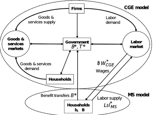
Figure 1 MS–CGE Integration
If the occupational levels calculated by the MS model are different from those in the CGE model, they change the equilibrium of the labor markets, which will then change wages and the economic environment as a whole until the CGE model reaches a new equilibrium. In this sense, step 2 restarts, but without changes in benefits and their financing sources, and this integrated solution procedure loops until the differences in the occupational level for all private labor types calculated by the MS model (Lsl*) approaches zero.21
This association is done consistently with the equilibrium of aggregate markets in the CGE model, which requires that: (i) relative changes in average earnings in the MS model must be equal to changes in wage rates from the CGE model for each private wage group in the labor market; (ii) relative changes in the number of privately waged workers by labor market segment in the MS model must match those in the CGE model; and (iii) changes in the consumption price vector, p, must be consistent with the CGE.22
According to the above procedure, the private labor supply is being modified with each simulation iteration; for example, some individuals will be losing their former jobs. If this happens, the share of each household in the total income of each labor category can also change (parameter hl in
equation 2.1.2). In order to capture these variations, we incorporate the differences among the parameter hl, along the simulation rounds as a shock in the CGE as well, which performs
simultaneously with the procedures described in this section.23
Goods & services markets Firms Government Households Labor market Households b, B Labor supply Labor demand Goods & services supply
Goods & services demand MS model CGE model Wages * MS Lsl * B * CGE W Benefit transfers * *,T B Goods & services markets Goods & services markets Firms Government Households Labor market Labor market Households b, B Labor supply Labor demand Goods & services supply
Goods & services demand MS model CGE model Wages * MS Lsl * B * CGE W Benefit transfers * *,T B
2.4. Non-Labor Income Procedures
After the CGE and MS models’ solutions converge, it is still necessary to treat non-labor incomes before calculating poverty and inequality indicators. Basically, the variables related to these sources of income in the MS model follow the CGE variations or maintain the same value as in the household survey, as shown in Table 3. In the former case, the changes from the CGE model are transmitted to the corresponding variables in the MS model in a unidirectional way.
Table 3: Integration of CGE-MS model for non-labor income (Base 2003)
Household Income Source Procedure in the Microsimulation (PNAD 2003)
Self Employed Income CGE results variations of these income sources are applied to the microsimulation model vectors.24
Interest, Dividends and Others and House Rental
CGE results variation of these income flows individualized to the 8 household categories in the model are applied to the microsimulation model vectors.25
Retiree and Pension
Public Benefits The same vector values as in the microsimulation base year model. Retiree and Pension
Private Benefits The same vector values as in the microsimulation base year model. Donation received The same vector values as in the microsimulation base year model.
Note: For each family, the above sources are deflated by a family specific price index (after simulation).26 Source: Authors’ elaboration.
3. SIMULATIONS AND RESULTS 3.1. Description of simulations
The direct aiming of the simulations is to assess the effects of changing values and beneficiaries of the programs PBF and BPC from the ones presented in 2003 to the ones presented in 2005.
Transfer Programs. We addressed the changes between 2003 and 2005 with similar procedures
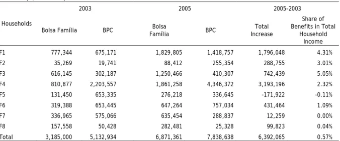
adopted by Barros et al. (2007c).27 However, we construct a specific imputation methodology for the 2005 additional benefits.28 Given this information, we then took the benefit share for the eight CGE household categories and apply the actual amounts given by Brazil’s budget data, ensuring consistency with our SAM data. The values are shown in Table 4.
Table 4: Total benefits by CGE household category and changes between 2003 and 2005
(R$ thousands)
Households
2003 2005 2005-2003
Bolsa Família BPC Bolsa
Família BPC Total Increase Share of Benefits in Total Household Income F1 777,344 675,171 1,829,805 1,418,757 1,796,048 4.31% F2 35,269 19,741 88,412 255,354 288,755 3.01% F3 616,145 302,187 1,250,466 410,307 742,439 5.05% F4 810,877 2,203,557 1,861,258 4,346,372 3,193,196 2.32% F5 131,450 653,335 276,218 336,645 -171,922 -0.11% F6 319,388 653,445 647,264 757,034 431,464 1.09% F7 336,965 575,066 635,454 288,837 12,259 0.00% F8 157,558 50,428 282,481 25,328 99,823 0.04% Total 3,185,000 5,132,934 6,871,361 7,838,638 6,392,065 0.57%
Source: Author’s elaboration based on data from the federal budget and SAM (2003).
The table above shows the differences in benefits between 2005 and 2003. Total transfers increased by R$6,392 million, which represents 0.57% of total household income. By program, the increase was approximately 116% for BF and 53% for BPC. Also, there was an overall improvement in the targeted group. The poorest households in the CGE model (F1, F2 and F3) increase their total BF share from 44.9% (2003) to 46.1% (2005). However, despite some improvements, the data show that the BPC targeting was much worse than the BF program (19.4% in 2003 and 26.6% in 2005).
We carried out two simulations, distinguished by whether the increased transfers are financed by public deficit (which reduces total savings and investment, according to the model’s macro closure) or increased taxes: SIMU A and SIMU B.
SIMU B: In this simulation, the increase in benefits is financed by increased federal government
taxes. This choice was made in order to hold the nominal public deficit almost constant. The main justification for this policy arrangement is the “Brazilian Fiscal Responsibility Law”, which states that new expenditures must be explicitly financed.
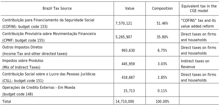
In order to replicate what happened in that period, we did an extensive analysis of the 2005 federal budget data to identify the specific tax sources that financed the PBF-BPC programs during that year. Table 5 summarizes the amounts of each federal tax source, their percentage composition, and the equivalent CGE tax as presented in the CGE model.
Table 5: Programs’ tax sources in 2005 (R$ thousands)
Brazil Tax Source Value Composition Equivalent tax in the CGE model Contribuição para Financiamento da Seguridade Social
(COFINS: budget code 153) 7,570,121 51.46%
“COFINS” tax and its value added reform Contribuição Provisória sobre Movimentação Financeira
(CPMF: budget code 155) 5,265,907 35.80%
Direct taxes on firms and households Outros Impostos Diretos
(Income Tax and other directed taxes) 993,630 6.75%
Direct taxes on firms and households Impostos sobre Produtos
(Mix of Indirect Taxes) 445,959 3.03%
Indirect taxes on Revenue Contribuição Social sobre o Lucro das Pessoas Jurídicas
(CSLL: budget code 151) 418,667 2.85%
Direct taxes on firms and households Operações de Credito Externas - Em Moeda
(budget code 148) 15,713 0.11%
Total 14,710,000 100.00%
Source: Authors’ elaboration.
From this table,29 we collected the share of each tax in the total increase of program expenditure (R$6,392,065,000). Thus, the following adjustments were made to the CGE model: (i) 2.2% increase in direct taxes on the gross income of the eight CGE household categories and firms; (ii) introduction of the Cofins tax through the replication of the PIS-COFINS tax reform, which was implemented by the federal government in the same period. From the total revenue generated by this reform, 27.5% was appropriated as funding for the cash transfer programs.
3.2. Macroeconomic impacts
Table 6 presents selected macro results for SIMU A and SIMU B. We first analyze SIMU B, which captures the combined effects of changes in transfers and taxes, while the results from SIMU A capture only the impacts of changes in transfers (and the public deficit).
In general, the macro impacts are adverse since they induce a real GDP fall of 0.46% and an aggregate employment decrease of 0.48%, while generating a price index increase of 0.65%. These adverse effects can mainly be attributed to the partial reform of PIS-COFINS that were the main tax sources of the transfer programs.
Table 6: Macroeconomic indicators (percentage change)*
Macroeconomics indicators SIMU A (%) SIMU B (%)
GDP –0.02 –0.46
Consumption 0.50 –0.35
Investment –1.42 –1.04
Public Sector Deficit +17.87 +7.38
Exports (**) –0.84
Imports (**) –1.07
Employment –0.11 –0.48
Price Index 0.13 0.65
Note: (*) Real percentage change from the CGE base year. (**) Lower than 0.01%. Source: Authors’ elaboration.
PIS-COFINS reform increases the taxation of firms’ value-added (VA), which leads to either higher marginal revenues or lower marginal costs through the reduction of VA components. Since capital is fixed by sector, this implies a lower labor demand, which induces a decrease in wages and, ultimately, household income. Specifically, the fall in aggregate consumption is due to the decrease in overall household income despite the rise of income among the poorest households who benefit most from the increase in transfers.
The taxation of imports increases their prices in the domestic market and induces another adverse effect on aggregate consumption, through higher domestic prices.
Exports fall due to the price-responsive behavior of external agents and the model’s external closure characteristics. First, the simulation induces an increase in domestic prices, which causes a decrease in external demand for Brazilian export goods. Second, since external macro closure implies a constant trade balance, the fall in imports must be accompanied by a fall in exports.
The government deficit increases by 7.88%, which shows that the ex-ante simulated taxation was not enough to completely finance the total transfer costs. Despite the “total financing” intention of SIMU B, the government deficit was not held constant because the taxes dead weight losses turn out to be very strong during the simulation.30
The comparison between SIMU A and SIMU B demonstrates the isolated effects of transfers without the tax increases. GDP in SIMU A is practically stable. However, the shock induces a trade-off between consumption and investment, with the former increasing by 0.5% and the latter decreasing by 1.42%. This fact can be explained by the increase in income transfer and by the higher public deficit (+17.89%), which reduces total savings. The consequent fall in investment will reduce economic growth in the near future, engendering additional negative effects not captured in this analysis. Therefore we can conclude that the adverse impacts of SIMU B are due
to the simulated program’s financing structure.
3.3. Impacts on Labor Market
SIMU B has an adverse effect on aggregate employment (-0.48%, according to Table 6). In SIMU A, the effect is small (-0.11%) but it is one of the few macro aggregates with negative impacts.
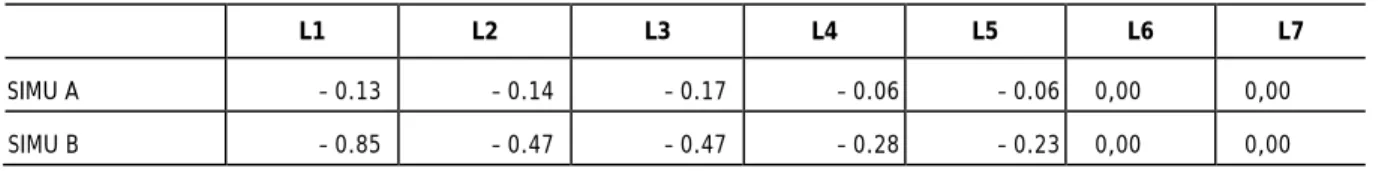
Table 7 shows that employment falls for all categories of workers in the private sector. The number of public worker does not change because, by model assumption and legal status, the quantities are fixed and the adjustments are done through flexible real wages.
Table 7: Change in employment from the base-year (%)
L1 L2 L3 L4 L5 L6 L7
SIMU A – 0.13 – 0.14 – 0.17 – 0.06 – 0.06 0,00 0,00
SIMU B – 0.85 – 0.47 – 0.47 – 0.28 – 0.23 0,00 0,00
Note: L1-unskilled informal; L2-skilled informal; L3-low-skilled formal; L4-average-skilled formal; L5- high-skilled formal; L6- low-skilled
public servants; L7- high-skilled public servants. Source: Authors’ elaboration.
In the SIMU B, among the private sector, we can see two patterns. The effects are more pronounced in the informal markets (L1 and L2) and among less skilled workers.
In our interpretation, with lower imports and a fixed trade balance, there is pressure to overvalue the real exchange rate making exports more expensive. The sectors in which exports are more sensitive to price changes are the most traditional ones, which are more intensive in informal and low-skilled workers. On the other hand, the fall of consumption in high income households affect the employment of more skilled workers in the sectors that produce goods with higher technological content, such as automobiles, auto parts, electronic, electrical, and pharmaceutical industries.
Table 8 show generally negative impacts on real wages by labor type. In the SIMU B, the wage of less skilled workers (L1 and L3) fall more than the other types. The reduction in public servants’ earnings is due to the model hypothesis stressed above.
Table 8: Change in the average real wage from the base-year (%)
L1 L2 L3 L4 L5 L6 L7
SIMU A + 0,32 – 0,12 – 0,04 – 0,07 – 0,09 – 0,04 – 0,01 SIMU B – 1,77 – 0.96 – 1,52 – 0,90 – 1,61 – 1,66 – 1,62
Note: L1-unskilled informal; L2-skilled informal; L3-low-skilled formal; L4-average-skilled formal; L5- high-skilled formal; L6- low-skilled
public servants; L7- high-skilled public servants. Source: Authors’ elaboration.
Table 9 shows the effects on the total labor income, combining wage and employment effects. These are stronger among the less skilled workers, especially for those in the informal market, and due mainly to real wage effects.
Table 9: Changes in real payroll from the base-year (%)
L1 L2 L3 L4 L5 L6 L7
SIMU A + 0,19 – 0,25 – 0,21 – 0,13 – 0,14 – 0,04 – 0,01
SIMU B –2.62 –1.43 –1.99 –1.18 –1.84 –1.66 –1.62
Note: L1-unskilled informal; L2-skilled informal; L3-low-skilled formal; L4-average-skilled formal; L5- high-skilled formal; L6- low-skilled
public servants; L7- high-skilled public servants. Source: Authors’ elaboration.
Again, SIMU A has practically no significant adverse effects. In contrast to SIMU B, informal unskilled workers (L1) fare better, due to the fact that there is a reallocation of production toward more labor-intensive sectors.
Finally, it is important to stress that the convergence procedures affect the final labor market equilibrium. Table 10 illustrates this process for SIMU B. The first line show changes in real wages, the price index and GDP in the first simulation round. In the second line, the same variables are presented for the last round. The convergence solution shows that changes in the transfer programs induce general equilibrium effects that initially affect wages primarily and then, due to the iterative process, are partially reallocated to employment impacts (quantity effects).
Table 10: Differences between first and last SIMU B rounds – selected variables
(%)
wage L1 wage L2 wage L3 wage L4 wage L5 pindex GDP First round simu B – 2,16 – 1,39 – 1,76 – 1,29 – 1,93 0.56 – 0.41 Last round simu B – 1,77 – 0.96 – 1,52 – 0,90 – 1,61 0,65 – 0,46
Source: Authors’ elaboration.
3.4. Impacts on Income Distribution
Table 11 shows the impacts of the changes in the transfer programs on inequality indicators. In general, the results confirm the important role of transfer programs in the fall in Brazil’s inequality during that period.31.
Table 11: Inequality indicators from household per capita income
(base year 2003)
Inequality Indicators
Base Year SIMU A SIMU B
Original Results** Change Results** Change
Gini Index 0.5930 0.5908 – 0.37% 0.5902 – 0.48%
Theil-T Index 0.7213 0.7163 – 0.69% 0.7161 – 0.72%
Source: from the CGE-MS integration model. (base year: 2003 PNAD survey)
Analyzing the Gini index, the fall of –0.48% (SIMU B) is slightly lower than the ones reported by other studies that evaluated the contribution of transfer programs to the fall in inequality using partial equilibrium or decomposition analysis. Barros et al. (2007c) found that 22.9% of the total Gini decrease between 2001 and 2005 was due to BF and BPC. In the same period, these authors reported a total decrease in the Gini index of –2.6%. Therefore, the decrease displayed in table 10 accounts for approximately 14% (SIMU A) and 19% (SIMU B) of the total fall in inequality during that period.
Here, it is important to stress some differences between our simulations and the study by Barros et
al. (2007c). The simulations capture the effects of changes in a shorter period, from 2003 to 2005,
in a general equilibrium environment. Although the period is different, we found evidence that the transfer programs alone (SIMU A) had lower effects on inequality than those reported by other studies. However, in the case of SIMU B, the effect is similar.
Table 12 shows the impacts on household income. The changes in programs have a slightly adverse effect on national average household income in SIMU A (-0.18 %), which is magnified (-0.81%) in SIMU B. In both, the positive effects on the three poorest household categories are primarily due to the increase in transfer amounts to them. On the other hand, the effects of the programs’ expansion on the richest households (F7 and F8) are already negative in the first simulation (SIMU A) and are magnified when the changes in taxation were considered. There are two important causes of these negative impacts. The first is related to labor income reported in the former section. The other can be attributed to the general price increase and its effect on non-labor income such as social security benefits and interest on fixed income investments.
Table 12: Change in household income from the base-year
(%)
Average household income
Original SIMU A SIMU B
Values (R$) Values (R$) Change Values (R$) Change
National average 432.36 431.59 -0.18% 428.84 -0.81% Household 1 (F1) 43.88 45.89 4.58% 45.76 4.28% Household 2 (F2) 70.20 74.90 6.70% 74.89 6.69% Household 3 (F3) 46.87 47.89 2.17% 47.78 1.94% Household 4 (F4) 166.42 168.19 1.06% 167.67 0.75% Household 5 (F5) 303.65 302.57 –0.36% 301.23 –0.80% Household 6 (F6) 191.94 192.31 0.19% 191.76 –0.09% Household 7 (F7) 696.64 693.84 –0.40% 689.33 –1.05% Household 8 (F8) 3,015.14 2,998.08 –0.57% 2,972.50 –1.41%
Note: F1 – poor urban households headed by active individuals; F2 – poor urban households headed by non-active individuals; F3 – poor rural households; F4 – urban households with low average income; F5 – urban households with medium income; F6 – rural households with medium income; F7 – households with high average income; F8 – households with high income.
Source: Authors’ elaboration.
The positive impacts of the program’s expansion on the poorest household category are better reflected by SIMU A. This simulation also captures systemic effects induced from these programs, as shown in sections 3.2 and 3.4. Besides that, SIMU B also shows the additional negative impact of the increase of taxation. This helps to understand the improvement of the Gini index in SIMU B in relation to the SIMU A. Aside from capturing the income increase of the poorest households, it also captures the fall in income of the richest households due to the increased taxation.
3.5. Impacts on Poverty
The effects on poverty are presented in table 13. Based on observed and simulated income per household head, we calculate three poverty indicators: Headcount index (P0), Poverty Gap (P1) and Severity of Poverty (P2). These indicators are calculated using the microsimulation model before and after simulations. The reference line values are from September 2005 estimated by Barros et al. (2007b) and deflated to 2003 with the IPCA (Índice de Preços ao Consumidor Amplo) price index.
Table 13: Poverty indicators - PNAD 2003
Poverty Indicators
Base year SIMU A SIMU B
Results* Results Change Results Change
Poverty Line (Line = R$ 143,70)
P0 0.3299 0.3256 –1.29% 0.3271 –0.84%
P1 0.1599 0.1579 –1.26% 0.1593 –0.38%
P2 0.1061 0.1047 –1.28% 0.1060 –0.08%
Extreme Poverty Lines (Line = R$ 71,84)
P0 0.1485 0.1473 –0.83% 0.1485 0.01%
P1 0.0777 0.0766 –1.38% 0.0778 0.18%
P2 0.0578 0.0569 –1.52% 0.0580 0.40%
Source: Authors’ elaboration.
The general reduction in poverty indicators (P0, P1 and P2) shows that the transfer programs alone (SIMU A) had positive effects on poverty and on extreme poverty. From the results in the table 13 we also see that the impacts on poverty were reduced by the changes in taxation (SIMU B). As discussed above, tax changes generate some adverse impacts that affect the poor population and, in a more intensive way, the extremely poor individuals. As we have seen previously in section 3.4, the impacts on labor income were stronger among the less skilled workers (L1 and L3) and the informal workers (L1 and L2). These workers are predominantly from the poorest households, which are highly dependent on labor income. Therefore, despite the increase in the received benefits, some households fall into poverty due to increased taxation.
In the case of SIMU B, the program expansion did not have an impact on extreme poverty. However, the poverty gap and severity of extreme poverty worsened. One explanation is the deterioration of non-labor income due to the price increase, which especially affected the family F2 located, before shock, just above the poverty line and whose income is basically derived from social security benefits.
4. CONCLUSIONS
The aim of the simulations presented here was to investigate the role of the two most important Brazilian cash transfer programs in reducing inequality. This was done through a CGE-microsimulation (CGE-MS) iterative approach. Two simulations were run, where the cost of increased transfers was financed by increased taxes or a rise in the public deficit.
The macro results showed that, in general, the impacts were adverse for several macro indicators, including GDP, employment, and price index. However, importantly, the study’s CGE-MS
framework brings out the fact that the adverse results came mainly from the tax increases and not the increase in transfers.
The results confirmed the important role of the PBF and BPC programs in the recent reduction in income inequality in Brazil. Practically 20% of the fall in inequality between 2003 and 2005 can be attributed to the adopted policies. These results are similar to those reported by other studies using partial equilibrium/decomposition analysis. However, again, this study’s CGE-MS framework reveals that the accompanying tax reform played a major role in this process.
The programs also contributed to a reduction in poverty. However, the impacts were smaller than for inequality. The transfers generated positive impacts, but the general equilibrium effects of the changes in taxation to finance the program largely offset the former effect, particularly in the case of extreme poverty indicators. Household income was effected through reduction in labor and non-labor income.
In general, the results also demonstrated that the two analyzed programs have achieved their objective of reducing poverty and inequality. However, the simulations showed that PBF targeted its beneficiaries better, concentrating its benefits on poor households.
Finally, it is clear that the financing of transfer programs plays an important role in the final welfare impacts. In our opinion, this issue deserves more attention in a policy research agenda.
ACKNOWLEDGEMENT
This work was carried out with financial and scientific support from the Partnership for Economic Policy (PEP), with funding from the Department for International Development (DFID) of the United Kingdom (or UK Aid), and the Government of Canada through the International Development Research Center (IDRC).
REFERENCES
Adelman I and Robinson S (1978) Income distribution policy in developing country: A case study of Korea. Stanford CA: Stanford University Press.
Agénor P R, Izquierdo A and Fofack H. (2001) ‘IMMPA: A Quantitative Macroeconomic Framework for the Analysis of Poverty Reduction Strategies’, Washington, D.C.: The World Bank (mimeo).
Armington P (1969) ‘A Theory of Demand for Products Distinguished by Place of Production’,
IMF Staff Papers, vol. 16, pp. 157-178.
de Barros R P, Carvalho M, Franco S and Mendonça R (2007a) ‘A Queda Recente da Desigualdade de Renda no Brasil’, in: de Barros R P, Foguel M N and Ulyssea G (eds.) Desigualdade de Renda
no Brasil: uma análise da queda recente. Brasília: Ipea, Vol. 1.
de Barros R P, Carvalho M, Franco S and Mendonça R (2007b) ‘A importância da queda recente da desigualdade para a Pobreza’, in: de Barros R P, Foguel M N and Ulyssea G (eds) Desigualdade
de Renda no Brasil: uma análise da queda recente. Brasília: Ipea, Vol. 1.
de Barros R P, Carvalho M and Franco S (2007c) ‘O papel das transferências públicas na queda recente da desigualdade de renda brasileira’, in: de Barros R P, Foguel M N and Ulyssea G (eds)
Desigualdade de Renda no Brasil: uma análise da queda recente. Brasília: Ipea, Vol. 2.
de Barros R P, Corseuil C H and Cury S (2000) ‘Salário mínimo e pobreza: uma abordagem de equilíbrio geral’, Pesquisa e Planejamento Econômico, Rio de Janeiro: IPEA, 30(2): 157-182.
de Barros R P, Foguel M N and Ulyssea G (2007d) Desigualdade de Renda no Brasil: uma análise da
queda recente. Brasília: Ipea, Vols. 1 e 2.
Becker G S (1965) ‘A Theory of Allocation of Time’, Economic Journal, 75:493-517.
Blanchflower D G and Oswald A J (1990) ‘The wage curve’, Scandinavian Journal of Economics, v.92, pp. 215-235.
Blanchflower D G and Oswald A J (1994) The wage curve. Cambridge, Massachussetts: MIT Press.
Blundell R and McCurdy T (1999) ‘A labour supply: a review of alternative approaches’, in: Ashenfelter O and Card D (eds.) Handbook of Labor Economics III, pp. 1559-1695. Amsterdam: North Holland.
Boccanfuso D, Cisse F, Diagne, A and Savard L (2003) ‘Un modèle CGE-Multi-Ménages Intégrés Appliqué à l’Économie Sénégalaise’, mimeo, CREA, Dakar.
Bonnet C and Mahieu R (2000) ‘Public pensions in a dynamic microanalytic framework: the case of France’, in: Mitton L, Sutherland H and Weeks M (eds) Microsimulation Modelling for Policy
Bourguignon F, Robilliard A S and Robinson S (2003) ‘Representative versus Real Households in the Macroeconomic Modeling of Inequality’, Working Paper, nº. 2003-05, DELTA/ENS, Paris.
Bourguignon F and Savard L (2008) ‘A CGE Integrated Multi-Household Model with Segmented Labour Markets and unemployment’, in: Bourguignon F, Pereira da Silva L A and Bussolo M (eds.), The Impact of Macroeconomic Policies on Poverty and Income Distribution: Macro-Micro Evaluation
Techniques and Tools, Palgrave-Macmillan Publishers Limited, Houndmills, England.
Chen S and Ravallion M (2004) ‘Welfare impacts of China’s accession to the world trade organization’, The World Bank Economic Review. 18(1): 29-57.
Chia N C, Wahba S and Whalley J (1994) ‘Poverty-Reduction Targeting Programs: a General Equilibrium Approach’, Journal of African Economies, 3(2), pp. 309-338.
Coady D P and Harris R L (2004) ‘Evaluating Targeted Cash Transfer Programs – A General Equilibrium Framework with an Application to Mexico’, Research Report 137, International Food Policy Research Institute, Washington, DC.
Cockburn J (2001) ‘Trade liberalization and Poverty in Nepal: A Computable General Equilibrium micro-simulation Analysis’, Working paper nº. 01-18. CREFA, Université Laval.
Cockburn J, Savard L and Tiberti L (2015) ‘Macro-Micro Models’, in: O'Donoghue C (2014) The
Handbook of Microsimulation Modelling, Emerald Group Publishing Limited.
Coelho A M, Corseuil C H, Cury S and de Barros R P (2003) ‘Um modelo de equilíbrio geral computável para analisar aspectos distributivos no Brasil’, in: Corseuil C H and Kume H (eds):
A Abertura Comercial Brasileira nos anos 90 – impactos sobre emprego e salário. Rio de Janeiro: IPEA,
pp. 171-197.
Colatei D and Round J I (2001) ‘Poverty and Policy: Some experiments with a SAM-Based CGE Model for Ghana’, Paper presented to the XIII International Conference on Input-Output Techniques, Macerata, Italy (August).
Covre S, Marques F and Mattos E (2008) ‘Oferta de trabalho e transferências: Evidências dos efeitos das condições impostas pelo programa Bolsa-Família’, ANPEC, available at
http://www.anpec.org.br/encontro2008/artigos/200807141223420-.pdf.
crescimento no Brasil’, PhD dissertation (Doutorado em Economia de Empresas) – Depto de Economia, Escola de Administração de Empresas de São Paulo, Fundação Getulio Vargas.
Cury S and Coelho A M (2006) ‘From revenue to value added taxes: welfare and fiscal efficiency effects in Brazil’, Proceedings of the International Conference on Policy Modeling (ECOMOD 2006), Hong Kong, June.
Cury S, Coelho A M and Pedrozo E (2006) ‘Matriz de Contabilidade Social - Brasil 2003’, Relatório de Pesquisa 461/04 (Anexo 1), São Paulo: GV Pesquisa, EAESP–FGV, fevereiro 2006, mimeo.
Cury S, Coelho A M and Corseuil C H (2005) ‘A Computable General Equilibrium Model to Analyze Distributive Aspects in Brazil with a Trade Policy Illustration’, Estudos Econômicos, São Paulo: IPE/FEA/USP, 35(4): 739-765.
Cury S, Pedrozo E, Coelho A M and Callegari I (2010) ‘The Impacts of Income Transfer Programs on Income Distribution and Poverty in Brazil: An Integrated Microsimulation and Computable General Equilibrium Analysis’, MPIA-PEP Working Paper 11086.
De Janvry A, Sadoulet E and Fargeix A (1991) Adjustment and Equity in Ecuador. Paris: OECD Development Center.
Decaluwé B, Patry A, Savard L and Thorbecke E (1999a) ‘Poverty Analysis within a General Equilibrium Framework’, Working Paper 99-09, African Economic Research Consortium.
Decaluwé B, Dumont J C and Savard L (1999b) ‘How to Measure Poverty and Inequality in General Equilibrium Framework’, Working Paper #9920, Laval University, CREFA.
Dervis K, de Melo J and Robinson S (1982) General Equilibrium Models for Development Policy. Cambridge University Press, London, pp. 1-526.
Devarajan S, Lewis J and Robinson S (1991) ‘From stylized to applied models: building multisector CGE models for models for policy analysis’, CUDARE Working Paper Series nº. 616, University of California at Berkeley, Dept. of Agricultural and Resource Economics and Policy.
Ferro A R and Nicollela A C (2007) ‘The impact of conditional cash transfer programs on household work decisions in Brazil’, in: Population Association of America 2007 Annual Meeting, Available at http://paa2007.princeton.edu/download.aspx?submissionId=71442.
conditional cash transfer programs’, EconomiA, 15(2014), pp. 243–260.
Foguel M N and de Barros R P (2008) ‘The Effects of Conditional Cash Transfer Programs on Adult Labour Supply: An Empirical Analysis Using a Time-Series-Cross-Section Sample of Brazilian Municipalities’, ANPEC, available at http://www.anpec.org.br/encontro2008/ artigos/200807211655420-.pdf.
Gronau R (1986) ‘Home Production – A Survey’, in: Ashenfelter O and Layard R (eds.) Handbook
of Labor Economics, vol. 1, chapter 4. Amsterdan: North Holland.
Gunning W J (1983) ‘Income Distribution and Growth: A Simulation Model for Kenya’, in: Greene D G (principal author) Kenya: Growth and Structural Change, 2 vols., Washington, DC: World Bank, pp. 487-621.
Heckman J (1974) ‘Shadow Prices, Market Wages, and Labor Supply’, Econometrica, nº. 42: 679-694.
Heckman J (1979) ‘Sample selection bias as a specification error’, Econometrica, nº. 47: 153-61.
Hoffmann R (2006a) ‘Brasil, 2004: Menos pobres e menos ricos’, in: Parcerias Estratégicas - Edição especial: Análise sobre a Pesquisa Nacional por Amostra de Domicílios (Pnad 2004). Brasília: Centro de Gestão e Estudos Estratégicos, nº. 22, p. 77–88.
Hoffmann R (2006b) ‘Transferências de renda e a redução da desigualdade no Brasil e cinco regiões entre 1997 e 2004’, Econômica. Rio de Janeiro, 8(1): 55-81.
IPEA (2012) ‘A Década Inclusiva (2001-2011): Desigualdade, Pobreza e Políticas de Renda’,
Comunicados IPEA, nº 155, Sept. 25, 2012, Brasília.
IPEA (2015) Boletim de Políticas Sociais - acompanhamento e análise nº 23, 2015. IPEA, 2015, Brasília.
King D and Handa S (2003) ‘The welfare effects of balance of payments reforms: A macro-micro simulation of the cost of rent-seeking’, The Journal of Development Studies 39(3): 101-128.
Müller T (2004) ‘Evaluating the economic effects of income security reforms in Switzerland: an integrated microsimulation - computable general equilibrium approach’, Working Paper, University of Geneva.
Brazil’, Estúdios de Economia, v. 21, p. 79-111.
Santos A H da Silva (2013) ‘Redução da Desigualdade Renda no Brasil: determinantes e consequências’, in: ESAF - VI Prêmio SOF de Monografias, 2013.
Savard L (2003) ‘Poverty and Income Distribution in a CGE-Household Micro-Simulation Model: Top-Down/Bottom-Up Approach’, CIRPRÉ – Centre Interuniversitaire sur le Risque, les Politiques Économiques et l’Emploi, Working Paper 03-43, 39 p.
Savard L (2005) ‘Poverty and inequality analysis within a CGE Framework: a comparative analysis of the representative agent and microsimulation approaches’, Development Policy Review, 23(3), 313-332.
Soares F V, Ribas R P and Osório R G (2007) ‘Avaliando o Impacto do Programa Bolsa Família: uma Comparacão com Programas de TransferênciaC ondicionada de Renda de Outros Países’, IPC Evaluation Note, No. 1. IPC, Brasília.
Tavares P A (2008) ‘Efeito do Programa Bolsa Família sobre a Oferta de Trabalho das Mães’, XIII Seminário sobre Economia Mineira – Economia, História, Demografia e Políticas Públicas, Diamantina – MG – Brasil, agosto de 2008.
Taylor L and Lysy F (1979) ‘Vanishing income redistributions: Keynesian clues about model surprises in the short-run’, Journal of Development Economics 6(1):11-29.
Teixeira C G (2008) ‘Análise do Impacto do Programa Bolsa Família na Oferta de Trabalho dos
Homens e Mulheres’, UNDP/IPC, Available at
http://www.ipc-undp.org/publications/mds/27P.pdf.
Vos R, De Jong N (2003) ‘Trade liberalization and poverty in Ecuador: a CGE macromicrosimulation analysis’, Economic System Research 15(2): 211-232.
1 See Barros et al. (2007a) and Hoffmann (2006a) for more details.
2 Recently, starting in 2014, Brazil experienced a severe macroeconomic crisis with GDP falling sharply.
Probably, this situation will result in a worsening of social indicators such as the poverty level.
3 These data were kindly provided by Samuel Franco from OPE Sociais (www.opesociais.com.br) and
Ricardo Paes de Barros from INSPER, based on the National Survey by Household Sampling (PNAD) from 2001 to 2014.
4 Henceforth they will be respectively referred as PBF and BPC. The full description and data for these
programs are presented in Cury et al. (2010, Appendix D).
5 IPEA (2015).
6 Cury et al. (2010, Appendixes A, B, C and D) supplement this article with the equations used in the CGE
model, intermediate results, and data on the transfer programs.
7 The CGE model used in this research is an extension of the one presented by Cury et al. (2005), where further details can be found, and is a result of a series of developments made in the model proposed by Devarajan et al. (1991), as can be seen in Cury (1998), Barros et al. (2000) and Coelho et al. (2003). 8 Poor urban families headed by an active individual (F1), poor urban families headed by a non-active
individual (F2), poor rural families (F3), urban families with low average income (F4), urban families with medium income (F5), rural families with medium income (F6), families with high average income (F7), and families with high income and a significant share of non-wage income (F8).
9 Unskilled informal (L1), skilled informal (L2), low-skilled formal (L3), average-skilled formal (L4), high-skilled formal (L5), low-high-skilled public servants (L6) high-high-skilled public servants (L7).
10 The SAM used in this research is fully described and documented by Cury et al. (2006), which can be requested from the authors.
11 See Appendix B in Cury et al. (2010) for database details.
12 The Brazilian labor market also has a segment of non-flexible wages. However, this segment is formed primarily by public sector workers with job stability clauses. These workers who belong to the factors L6 and L7 are not included in the MS model, but they are agents on CGE model.
13 In Savard (2003), the labor market is segmented in two types: one with a fixed wage and another one with a flexible wage. Therefore, an individual could alter across three states (observing the implicit costs of choosing each one of them): offering her workforce in each one of the two markets or getting unemployed by choice.
14 We do not use a household labor supply model that is based on a family joint decision due to various difficulties in identifying the domestic production function (Becker, 1965) from the PNAD data. In this case, we followed the recommendation of Gronau (1986) where the lack of domestic production data should be replaced by family characteristics (such as all types of income) and demographic aspects. 15 This functional form was proposed because it is consistent with 1) the existence of individuals’
preferences by labor and leisure, and 2) the presence of households’ budget constraints (Blundell and McCurdy, 1999).
16 The first part of the microsimulation process is the computation of the labor supply equation (2.2.1). The entire PNAD sample was considered for this phase. Table B.3 in Cury et al. (2010) contains the overall heckit estimates by the system equation, including the coefficients and their standard errors to 5 percent of significance, as well as the inverse of the Mills’s ratio.
17 Equations 2.2.1 and 2.2.2 determine the working hours potentially supplied according to individual characteristics (see step 1).
18 For this phase, only private sector workers are considered. Table B.4 in Cury et al. (2010) contains the econometric estimates of this system of equations and the benefits shocks, changing the log Bi that corresponds to the PBF and BPC amounts of 2003, to log B*I, which corresponds to the benefits amounts of 2005.The procedure to impute these values in the 2003 database is described in Appendix C