Escola de Engenharia Departamento de Inform´atica
H´elder Jos´e Alves Gonc¸alves
Towards an efficient lattice basis
reduction implementation
Escola de Engenharia Departamento de Inform´atica
H´elder Jos´e Alves Gonc¸alves
Towards an efficient lattice basis
reduction implementation
Master dissertation
Master Degree in Computer Science
Supervisor: Alberto Jos ´e Proenc¸a
External Advisor: Artur Miguel Matos Mariano
Quero agradecer ao meu orientador, Alberto Proenc¸a, por todo o esforc¸o despendido para a realizac¸˜ao desta dissertac¸˜ao, em que o seu acompanhamento constante e rigor exigido foram imprescind´ıveis. Tamb´em quero agradecer ao meu orientador externo, Artur Mari-ano, pela oportunidade de efectuar um est´agio no ˆambito da dissertac¸˜ao na Alemanha.
I would also like to thank the Institute for Scientific Computing for receiving me in Darm-stadt. A special thanks to F´abio Correia for every discussions on the subject or not, during my internship. I also would like to thank Professor Christian Bischof, Florian G ¨opfert and Dominique Metz.
I would also like to acknowledge Professor Shizhang Qiao and Rui Ralha for all sugges-tions.
Tamb´em quero agradecer aos meus colegas de curso e amigos F´abio Gomes e Duarte Duarte pelo ajuda dada na revis˜ao da escrita da dissertac¸˜ao e por todas as conversas fant´asticas que se sucederam no Skype durante este ´ultimo ano.
Um especial obrigado `a M´arcia Couto por todo o suporte dado durante este ´ultimo ano. Finamente mas n˜ao menos importante, quero agradecer aos meus pais por todo o suporte, esforc¸o e dedicac¸˜ao prestados n˜ao s ´o neste ´ultimo ano mas por todos os anos que me trouxeram a este ponto.
The security of most digital systems is under serious threats due to major technology break-throughs we are experienced in nowadays. Lattice-based cryptosystems are one of the most promising post-quantum types of cryptography, since it is believed to be secure against quantum computer attacks. Their security is based on the hardness of the Shortest Vector Problem and Closest Vector Problem.
Lattice basis reduction algorithms are used in several fields, such as lattice-based cryp-tography and signal processing. They aim to make the problem easier to solve by obtaining shorter and more orthogonal basis. Some case studies work with numbers with hundreds of digits to ensure harder problems, which require Multiple Precision (MP) arithmetic. This dissertation presents a novel integer representation for MP arithmetic and the algorithms for the associated operations, MpIM. It also compares these implementations with other li-braries, such as GNU Multiple Precision Arithmetic Library, where our experimental results display a similar performance and for some operations better performances.
This dissertation also describes a novel lattice basis reduction module, LattBRed, which included a novel efficient implementation of the Qiao’s Jacobi method, a Lenstra-Lenstra-Lov´asz (LLL) algorithm and associated parallel implementations, a parallel variant of the Block Korkine-Zolotarev (BKZ) algorithm and its implementation and MP versions of the the Qiao’s Jacobi method, the LLL and BKZ algorithms.
Experimental performances measurements with the set of implemented modifications of the Qiao’s Jacobi method show some performance improvements and some degradations but speedups greater than 100 in Ajtai-type bases.
Atualmente existe um grande avanc¸o tecnol ´ogico que poder´a colocar em causa a seguranc¸a da maioria dos sistemas inform´aticos. Sistemas criptogr´aficos baseados em reticulados s˜ao um dos mais promissores tipos de criptografia p ´os-quˆantica, uma vez que se acredita que estes sistemas s˜ao seguros contra poss´ıveis ataques de computadores quˆanticos. A seguranc¸a destes sistemas est´a baseada na dificuldade de resolver o problema do vetor mais curto e o problema do vetor mais pr ´oximo.
Algoritmos de reduc¸˜ao de bases de reticulados s˜ao usados em muitos campos cient´ıficos, tais como criptografia baseada em reticulados. O seu principal objetivo ´e tornar o prob-lema mais f´acil de resolver, tornando a base do reticulado mais curta e ortogonal. Al-guns casos de estudo requerem o uso de n ´umeros com centenas de d´ıgitos para garantir problemas mais dif´ıceis. Portanto, ´e importante o uso de m ´odulos de precis˜ao m ´ultipla. Esta dissertac¸˜ao apresenta uma nova representac¸˜ao de inteiros para aritm´etica de precis˜ao m ´ultipla e todas as respetivas func¸ ˜oes de um m ´odulo, ‘MpIM’. Tamb´em comparamos as nossas implementac¸ ˜oes com outras bibliotecas de precis˜ao m ´ultipla, tais como ‘GNU Multi-ple Precision Arithmetic Library’, em que obtivemos desempenhos semelhantes e em alguns casos melhores.
A dissertac¸˜ao tamb´em apresenta um novo m ´odulo para a reduc¸˜ao de bases de reticulados, ‘MpIM’, que inclui uma nova e eficiente implementac¸˜ao do ‘Qiao’s Jacobi method’, o algoritmo ‘Lenstra-Lenstra-Lov´asz’ (LLL) e respectiva implementac¸˜ao paralela, uma variante paralela do algoritmo ‘Block Korkine-Zolotarev’ (BKZ) e a sua vers˜ao sequencial e vers ˜oes the precis˜ao m ´ultipla do ‘Qiao’s Jacobi method’, LLL e BKZ.
Trabalhos experimentais mostraram que a vers˜ao do ‘Qiao’s Jacobi method’ que implementa todas as modificac¸ ˜oes sugeridas mostra ganhos e degradac¸ ˜oes de desempenho, contudo com aumentos de desempenho superiores a 100 vezes em bases ‘Ajtai-type’.
1 i n t r o d u c t i o n 2 1.1 Motivation 4 1.2 Contribution 4 1.3 Roadmap 4 2 b a c k g r o u n d a n d s e t u p 6 2.1 Multiple precision 7 2.1.1 Current libraries 7 2.1.2 Integer Representation 9
2.1.3 Addition and Subtraction 11
2.1.4 Multiplication 12
2.1.5 Division 17
2.1.6 Newton’s method 19
2.1.7 Hensel’s division 20
2.2 Lattice basis reduction 21
2.2.1 Basic Concepts 22
2.2.2 Lenstra–Lenstra–Lov´asz 24
2.2.3 Hermite-Korkine-Zolotarev 26
2.2.4 Block-Korkine-Zolotarev 26
2.2.5 Qiao’s Jacobi method 28
2.2.6 Measuring Basis Quality 30
2.3 Experimental environment 31
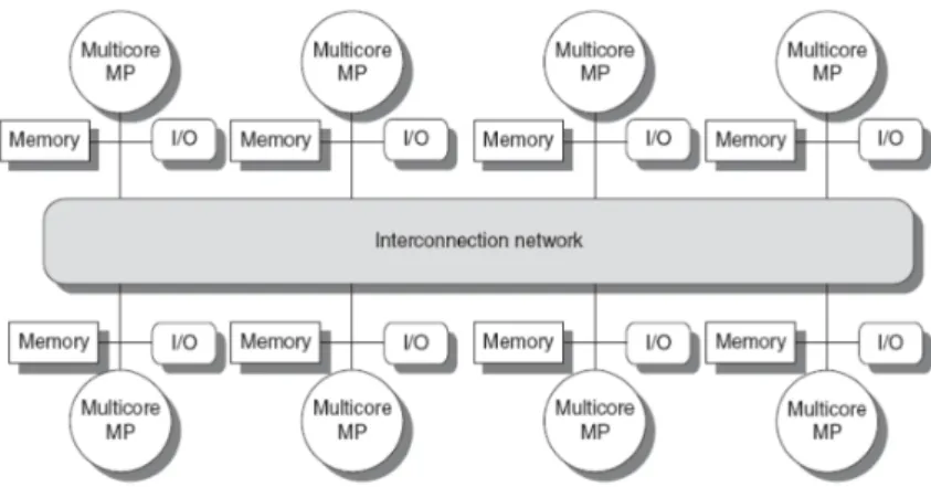
2.3.1 Non-Uniform Memory Access 31
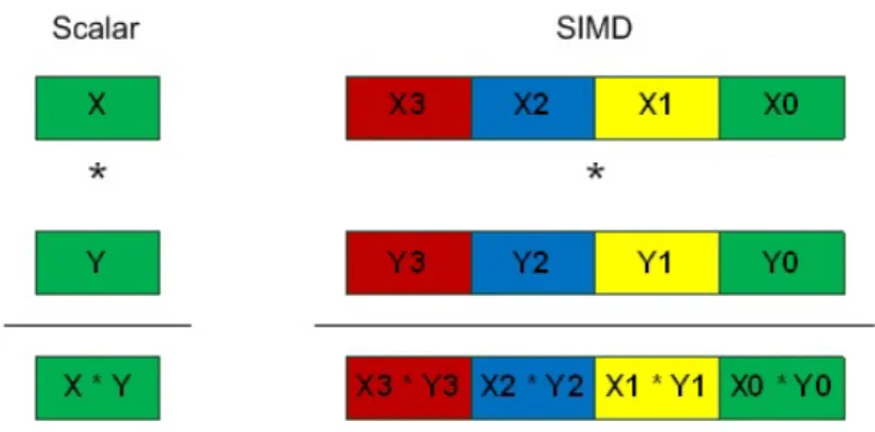
2.3.2 Vectorization 33
2.3.3 Methodologies 33
3 t h e m u lt i p l e p r e c i s i o n i n t e g e r m o d u l e 35
3.1 Addition and Subtraction 35
3.1.1 Addition Vectorization 36
3.1.2 Increment and Decrement 36
3.2 Multiplication 37 3.2.1 Long multiplication 37 3.2.2 Karatsuba 38 3.3 Division 39 3.4 Other Functions 39 3.4.1 Logical Shifts 39 iv
3.4.2 And/Or/Xor 42
3.4.3 Pseudo-Random Number Generator 42
3.4.4 Compare 42 3.5 Evaluation Results 43 4 t h e q i a o’s jacobi method 48 4.0.1 Vectorization 50 4.0.2 Evaluation Results 51 4.1 Parallel Version 54 4.1.1 Evaluation Results 56
4.2 Basis Quality Assessment 57
5 b k z, lll and qiao’s jacobi method 60
5.1 Towards parallel approaches 60
5.1.1 Parallel LLL algorithm 60
5.1.2 Parallel BKZ algorithm 62
5.2 BKZ w/ Qiao’s Jacobi method 63
5.3 Reducing L-reduced bases 63
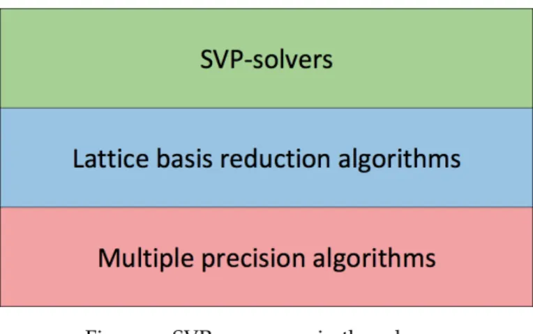
Figure 1 SVP panorama in three layers 6
Figure 2 Binary representation of a large number with 3 limbs. 10
Figure 3 Addition with a carry digit in a large number with 2 limbs. 11
Figure 4 The best algorithm to multiply two numbers of x and y limbs. bc is long multiplication, 22 is Karatsuba’s algorithm and 33, 32, 44 and 42are Toom variants (from [Brent and Zimmermann(2010)]). 13
Figure 5 Long multiplication algorithm (from Intel documentation). 14
Figure 6 Multiplication step (from Intel documentation). 14
Figure 7 Lattice reduction in two dimensions: the black vectors are the given basis for the lattice, the red vectors are the reduced basis (from
Wikipedia). 21
Figure 8 The first two steps of the Gram–Schmidt orthogonalization (from
Wikipedia). 23
Figure 9 Examples of GM matrices. 24
Figure 10 Chess tournament with n=8 (from [Jeremic and Qiao(2014)]). 29
Figure 11 Shared memory system (from Google Images). 32
Figure 12 One possible architecture of a NUMA system (from Advanced
Ar-chitectures slides). 32
Figure 13 Scalar implementation vs vector implementation (from Google
Im-ages). 33
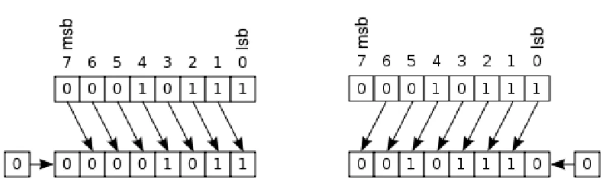
Figure 14 Simple logical right shift with the insertion of a zero on the left. 40
Figure 15 Simple logical left shift with the insertion of a zero on the right. 40
Figure 16 Right shift of 2 in a 3-limb large number. 40
Figure 17 Left shift of 2 in a 3-limb large number. 41
Figure 18 Comparison between the 5 addition implementations of the MpIM. 43
Figure 19 Comparison of MpIM’s addition to other libraries. 43
Figure 20 Comparison of MpIM’s subtraction to other libraries. 44
Figure 21 Comparison between the long multiplication and the Karatsuba
im-plementations of the MpIM. 44
Figure 22 Comparison of MpIM’s multiplication to other libraries. 44
Figure 23 Comparison of MpIM’s division to other libraries. 45
Figure 24 Comparison of MpIM’s right shift to other libraries. 46
Figure 25 Comparison of MpIM’s left shift to other libraries. 46
Figure 26 Comparison of MpIM’s ’or’ function to other libraries. 46
Figure 27 Comparison of MpIM’s ’and’ function to other libraries. 46
Figure 28 Comparison of MpIM’s ’xor’ function to other libraries. 47
Figure 29 Execution times of sequential LLL XD and Qiao’s Jacobi method in
GM bases. 52
Figure 30 Execution times of sequential LLL FP and Qiao algorithm in
Ajtai-type bases. 53
Figure 31 Number of necessary sweeps to converge to a solution in Ajtai-type
bases. 53
Figure 32 Speedups comparison between sequential LLL and Qiao’s Jacobi method
implementations in Ajtai-type bases. 54
Figure 33 Number of necessary sweeps to converge to a solution in GM bases. 55
Figure 34 Execution times of first parallel approach in GM bases. 57
Figure 35 Execution times of second parallel approach in GM bases. 57
Figure 36 Hermite factor of output basis from LLL algorithm and Qiao’s Jacobi
method in Ajtai-type bases. 59
Figure 37 Average of the norms of the output basis from LLL algorithm and Qiao’s Jacobi method in Ajtai-type bases. 59
Figure 38 Sequence of the GS norms from LLL algorithm and Qiao’s Jacobi
method in Ajtai-type bases. 59
Figure 39 Last GS norms from LLL algorithm and Qiao’s Jacobi method in
Ajtai-type bases. 59
Figure 40 Execution times of the Qiao’s Jacobi Method, the LLL and BKZ
algo-rithms. 63
Figure 41 Hermite factor of output basis from LLL and BKZ algorithms and
Qiao’s Jacobi method. 64
Figure 42 Average of the norms of output basis from LLL and BKZ algorithms
and Qiao’s Jacobi method. 64
Figure 43 Sequence of the GS norms of the output bases from the LLL and BKZ algorithms and the Qiao’s Jacobi method. 65
Figure 44 Last GS norms of output basis from LLL and BKZ algorithms and
2.1 Integer Addition, presented in [Brent and Zimmermann(2010)]. . . 12
2.2 Long Multiplication, presented in [Brent and Zimmermann(2010)]. . . 14
2.3 Karatsuba’s Algorithm, presented in [Brent and Zimmermann(2010)]. . . 15
2.4 Toom-Cook 3-Way Algorithm, presented in [Brent and Zimmermann(2010)]. 16 2.5 Long Division, presented in [Brent and Zimmermann(2010)]. . . 18
2.6 Long division (binary version), from Wikipedia. . . 19
2.7 Division By a Limb, presented in [Brent and Zimmermann(2010)]. . . 20
2.8 LLL algorithm, presented in [Nguyen and Stehl´e(2006)]. . . 25
2.9 BKZ algorithm, presented in [Chen and Nguyen(2011)]. . . 27
2.10 Qiao’s Jacobi Method, presented in [Qiao(2012)]. . . 29
3.1 Integer Increment . . . 37
4.1 Proposed Qiao’s Jacobi method . . . 49
5.1 Gram-Schmidt process for k . . . 61
1
I N T R O D U C T I O N
For years the cryptography community has been searching for more resistant cryptosys-tems. However, only in last decades there have been an intensive search for cryptosystems that would be resistant against quantum computers attacks. This necessity is explained by the vulnerability of the current popular cryptosystems, whose security relies on (i) the integer factorization problem, (ii) the discrete logarithm problem or (iii) the elliptic-curve discrete logarithm problem. Unfortunately, these three hard mathematical problems are no longer hard to solve on a sufficiently large quantum computer running Shor’s algorithm [Shor(1997),Bernstein(2009)].
Nowadays, lattice-based cryptosystems are one of the most promising post-quantum types of cryptography, due to its inherent computational hardness and fully-homomorphic properties. Lattices are rich algebraic structures that have many applications in computer science, namely integer programming [Kannan(1983)], communication theory [Agrell et al.
(2002),Nguyen (2010)] and number theory [Cassels(2012),Siegel(2013)].
The security of these cryptographic techniques is based on very strong security proofs based on the hardness of worst-case problems. Thus, breaking a cryptographic construction is probably at least as hard as solving several lattice problems in the worst-case.
Most current computer architectures support operations between numbers with up to 64 bits of precision. However, there are cases in cryptography where numbers with hundreds of digits (that cannot be represented as primitive data types) are required to ensure harder problems. Therefore, it is important to resort to Multiple Precision (MP) arithmetic to solve this kind of problems.
The bold face is used to represent vectors and matrices in this dissertation, where vectors are in lower-case and matrices are in upper-case, e.g., vector v and matrix M. The transpose of a matrix is given by MT and the dot product of two vectors v and p is denoted byhv, pi. Finally, dac rounds the value a to the nearest integer number and |a| gives the absolute value of a.
Lattices are simple algebraic structures based on familiar concepts to any user with basic training in algebra. The conceptual simplicity of these cryptographic techniques is associ-ated with simple matrix computations. A latticeLinRnis generated for all possible linear
combinations with integer coefficients of any basis inRn, where a basis B is a set of linear independent vectors(b1, ..., bn)and Z are all possible linear combinations, given by:
L =BZ= n
∑
i=0
bizi, zi ∈Z (1)
Take a latticeLembedded in a metric vector spaceA. SinceLis contained inA, there is the notion of size kxkand the notion of distancekx−zk, where x, z∈ L. These notions are enough to define two basic problems in lattices.
The Shortest Vector Problem (SVP) [Hanrot et al. (2011b)] can be informally defined as
the search for the shortest vector of a given latticeLand formally defined as follows: given a basis B for a lattice L = L(B), find a vector v ∈ L such that kvk = λ1(L), where the norm of the shortest vector of the lattice Lis given by λ1(L). In its approximated version (α-SVP), the goal is to search for that vector, this time multiplied by a small α factor1 2. On
the other hand, the Closest Vector Problem (CVP) is defined as follows: given a basis B for a lattice L = L(B)and a vector x ∈ Rn, find a vector v ∈ L such that kx−vk is minimal. The CVP and SVP problems are closely related.
The efficiency of several classes of algorithms that solve the SVP, such as enumeration, sieving and random sampling algorithms, is inherently connected with the quality of the input basis. Therefore, the development of new algorithms and the proposal of implemen-tations that improve the quality of a basis is imperative.
Nowadays, lattice enumeration algorithms are one of the main techniques to solve hard lattice problems such as SVP. A basic enumeration consists on an exhaustive search for the best combination of basis vectors among all others, leading to a run in exponential time executions.
In order to have a polynomial complexity algorithm we have to limit the algorithm spec-ification to do not necessarily require the shortest vector of the lattice but only a reduced basis. It is here that lattice basis reduction algorithms play an important role, where its goal is to transform a given basis B of a lattice L into a close to orthogonal and shorter basis such thatLremain the same. Since the reduced basis is shorter and more orthogonal, the SVP-solvers are capable of solve the SVP in less time, which compensate in most of the cases.
Lattice basis reduction algorithms are used in several applications, not only in the SVP. They have also been used in signal processing applications, such as Global Positioning Sys-tem (GPS), color space estimation in JPEG pictures, frequency estimation, and particularly data detection and precoding in wireless communications [Wbben et al. (2011),Tian and Qiao(2013)].
1 Lattice challenge -https://www.latticechallenge.org
1.1 m o t i vat i o n
Lattice-based cryptography has been a hot topic in the past 10 years, because systems based on lattices are believed to be secure against quantum computer attacks. These systems are based on the hardness of the SVP in theory, and of α-SVP in practice. While the SVP has been formulated more than a century ago, the algorithmic study of lattices started only in the early eighties, and the development of parallel algorithms for the SVP is even more recent, with developments in the last five years.
Despite the theoretical and practical hardness of the SVP, it is important to keep searching for new more efficient implementations or algorithms to prove that a particular problem may be easier to solve than the expected. The constant scrutiny of these problems is cru-cial to the scientific community, where a particular problem may be considered reliable or not. Thus, this dissertation focuses on lattice basis reduction algorithms and one of its key requirement, MP arithmetic.
1.2 c o n t r i b u t i o n
The work developed during this dissertation targeted performance improvements on lattice basis reduction techniques that lead to scientific contributions. These include:
• Development of an efficient ’Multiple precision Integer Module’ (MpIM)3
with mathe-matical operations, namely addition, increment, subtraction, decrement, multiplica-tion, division, left and right shifts, and several logical operations;
• Development of a ’Lattice Basis Reduction’ (LattBRed)3module. These include:
– A novel efficient implementation of the Qiao’s Jacobi method; – Parallel and MP versions of the Qiao’s Jacobi method;
– MP implementations of the LLL and BKZ algorithms.
• A basis quality assessment of the LLL algorithm and Qiao’s Jacobi method for Ajtai-type and Goldstein and Mayer lattice basis.
1.3 r oa d m a p
This dissertation is structured in six chapters. The first chapter introduces the reader the theme of this dissertation, and briefly explains the relevance of this topic for the scientific community.
The next chapter describes the necessary background to quickly understand the main subjects related to lattice basis reduction and describes the computational environment for the experimental work. The current approaches for MP and lattice basis reduction algorithms are presented in this chapter.
Chapter 3 presents the implemented MP operations and compares the module perfor-mance with existing libraries.
Chapter 4 is dedicated to the Qiao’s Jacobi method. It discusses the performance results achieved with the sequential and parallel versions of the algorithm and assesses a lattice basis quality of the Qiao’s Jacobi method.
Chapter 5 describes proposed parallel approaches of the LLL and BKZ algorithms and assesses the quality of the output basis of combining the LLL and the BKZ algorithm with the Qiao’s Jacobi method.
Finally, chapter 6 concludes the dissertation taking into account the obtained results, and leave guidelines for future work that could not be finished or covered.
2
B A C K G R O U N D A N D S E T U P
An SVP-solver searches the shortest non-zero vector of a latticeL. However, they used to be high complexity algorithms and they may run in exponential execution times. Some lattice basis reduction algorithms produce reduced basis in polynomial time [Lenstra et al.
(1982a)], but they do not solve the problem. The community have been doing a great effort
in the last years in SVP-solvers and lattice basis reduction algorithms, in order to get more efficient solutions. SVP-solvers are a class of techniques that solve the SVP. Enumeration, sieving and random sampling algorithms are three of the main techniques in SVP-solvers.
Figure 1: SVP panorama in three layers
Figure1illustrates a SVP panorama that this dissertation addresses. It splits the SVP into
three different layers.
SVP-solvers and lattice basis reduction algorithms can be used as stand alone algorithms, however they perform better together. The ’SVP-solvers’ layer is on the top because these algorithms always return the shortest non-zero vector of the lattice. Although the lattice basis reduction algorithms can solve the SVP for small basis dimensions, usually they only get a reduced basis which can then be used by a SVP-solver. Thus, they are below the layer ’SVP-solvers’. Finally, Multiple precision algorithms are in the bottom layer because they are used in both upper layers to represent and perform computations on large numbers that are inherit to the problem. Thus, this layer can be consider as support of the others. The dissertation is focused on the two lower layers.
2.1 m u lt i p l e p r e c i s i o n
Most current computer architectures support operations between integer scalars with up to 64 bits of precision. However, lattices in cryptography require numbers with a larger precision to ensure a better security in some applications. MP arithmetic requires the rep-resentation and computation of numbers that do not fit into primitive data types. With this approach it is possible to store and perform calculations on numbers whose precision digits are only limited by the available system memory.
Operations with primitive data types, whose numbers fit into processor registers, are considerably faster than the MP arithmetic. While primitive data types are implemented by hardware, MP arithmetic has to be implemented by software.
The MP history starts with a commercial IBM computer in the 50s1
. Unlike the current MP, implemented by software, the IBM 702 implemented a integer arithmetic entirely in hardware on digit strings up to 511 digits. Later in the 60s appear the first widespread software MP implementation in MACLISP (a dialect of the Lisp programming language). Already in the 80s, the VAX/VMS and VM/CMS were the first operating systems to offer MP functionalities.
This dissertation is focused in MP integer arithmetic, thus the algorithms here presented are intended to handle large integer numbers.
2.1.1 Current libraries
Current MP libraries are available for many programming languages. Languages such as Ruby and Haskell offer built-in support, but its performance decreases. In C and C++, one of the most used libraries is the GNU Multiple Precision Arithmetic Library (GMP)2
. GMP is a free library for MP arithmetic that was first released in 1991, and it has been updated since then. This library aims to have better implementations than any other MP library, mainly because it (i) uses full words to represent a large number, (ii) uses differ-ent algorithms for differdiffer-ent operand sizes since the algorithm efficiency depends on the operand, (iii) is specialized for different processor architectures with highly optimized as-sembly code, and (iv) is continuously updated by the worldwide community.
The Number Theory Library (NTL) is other widely used MP library3
. Unlike GMP that only implements MP modules, NTL has a strong component in number theory providing data structures and algorithms (e.g. routines for lattice basis reduction, Gaussian elimina-tion). It makes it way more attractive than GMP when the the research target goes beyond performance. The NTL author considers it a high-performance library and to increase its
1 Arbitrary precision arithmetic -https://en.wikipedia.org/wiki/Arbitrary-precision_arithmetic
2 GMP -https://gmplib.org
performance when using MP integer arithmetic, the author recommends to compile NTL with GMP. It also compares the relative performance of NTL against a similar library [Shoup
(2016)].
Class Library for Numbers (CLN) is a MP library for efficient computations4
. It stands out of the two previously libraries with a rich set of number classes, e.g., rational and com-plex numbers. As most high-performance libraries, it is implemented with C++ which brings efficiency, algebraic syntax and type safety. The CLN’s author claims that it is very efficient in MP integer arithmetic with the use of the Karatsuba algorithm [Karatsuba and Ofman (1962), Karatsuba (1995), Knuth (1997)] and the Fast Fourier Transform (FFT)
method [Sch ¨onhage and Strassen(1971)]. As most MP libraries, CLN is also dependent of
the GMP.
The previous MP libraries were consider for further experimental work to this disserta-tion due to its performance and MP number type. However, some well rated libraries were not considered for further experimental work, namely Multiple-Precision FP computations with correct Rounding library (MPFR)5
[Fousse et al. (2007)], Modular-positional
Floating-point format (MF-format) [Isupov and Knyazkov(2015)], Multiple Precision Integers and
Rationals library (MPIR)6
, Boost7
, Multiple Precision Floating-point Interval library (MPFI)8
[Revol and Rouillier(2005)], MPFUN20159, ARPREC10, GNU Multiple Precision Complex
library (MPC)11
, GNU Multi-Precision Rational Interval Arithmetic library (MPRIA)12
and Computer Algebra System (PARI/GP)13
. The exclusion of these libraries had several rea-sons: (i) their main functionalities are not relevant in the case study (e.g floating-point arithmetic, complex numbers, interval arithmetic and others), and (ii) several problems occurred when used (e.g. setup or segmentation fault problems and only beta releases).
In addition to these libraries others were also excluded because (i) we could not find rel-evant information about them, (ii) we assumed that their performance was lagging behind since they were not updated for several years or benchmarks showed that there are more ef-ficient libraries, and (iii) the target programming language is not C/C++. The list include Fast LIbrary for Number Theory (FLINT)14
, TTMath Bignum Library (TTMath)15
, Arbitrary 4 CLN -http://www.ginac.de/CLN/ 5 MPFR -http://www.mpfr.org 6 MPIR -http://mpir.org 7 Boost -http://www.boost.org 8 MPFI -http://mpfi.gforge.inria.fr 9 MPFUN2015 -http://www.davidhbailey.com/dhbsoftware 10 ARPREC -http://crd-legacy.lbl.gov/~dhbailey/mpdist/ 11 MPC -http://www.multiprecision.org 12 MPRIA -https://www.gnu.org/software/mpria/ 13 PARI/GP -http://pari.math.u-bordeaux.fr 14 FLINT -http://www.flintlib.org 15 TTMath - http://www.ttmath.org
precision library (ApFloat)16
, LibTomMath17
, CORE Library (CORE)18
[Du et al.(2002)],
eX-act Reals in C (XRC)19
, Multiple-precision Math (MpMath)20
, Software Carry-Save multiple-precision Library (SCSLib) [Defour et al.(2002),Defour and de Dinechin (2003)],
Floating-point Arithmetic Library (FpALib)21
, Supporting High Precision on Graphics Processors (GARPREC)22
, CudA Multiple Precision ARithmetic librarY (CAMPARY)23
, General Dec-imal Arithmetic Specification (MPDecDec-imal)24
, a Multi-precision Number Theory package (MpNT) [Hritcu et al.(2014),Tiplea et al. (2003)], Piologie25 , BigDigits multiple-precision
arithmetic (BigDigits)26
, C for eXtended Scientific Computing (C-XSC) [Hofschuster and Kr¨amer (2004)], Multiple precision Integer and Rational Arithmetic C Library (MIRACL)27
[Scott(2016)], My Arbitrary Precision Math library (MAPM)28[Ring(2001)]and simple and
complete bignum C library (bigz)29
.
2.1.2 Integer Representation
To represent MP numbers, it is necessary to create a structure that supports all computa-tions. The structure must allow efficient computations over the data.
The Residue Number System (RNS) was created by Sun Tsu Suan-Ching in the 4thcentury. The RNS is based in the Chinese remainder theorem for its operations. It uses a set of small numbers that fit in the primitive data types to represent a large MP number. As a large MP number is composed of a set of smaller numbers, a MP operation can be performed by compute in parallel and independently each small number.
However, RNS have some limitations, such as the division operation and the compari-son of numbers in order to improve the RNS performance several works have been done [Kaltofen and Hitz (1995), Chren (1990), Isupov and Knyazkov (2015)]. RNS cannot
effi-ciently compare two numbers: it has to convert those numbers to other representation to know, for example, which one is greater. To know more about this representational system see [Omondi and Premkumar(2007)].
16 ApFloat -http://www.apfloat.org 17 LibTomMath -http://www.libtom.net 18 CORE -http://cs.nyu.edu/exact/core_pages/intro.html 19 XRC -http://keithbriggs.info/xrc.html 20 MpMath -http://mpmath.org/ 21 FpALib -https://sourceforge.net/projects/precisefloating/ 22 GARPREC -https://code.google.com/archive/p/gpuprec/ 23 CAMPARY -http://homepages.laas.fr/mmjoldes/campary/ 24 MPDecimal -http://www.bytereef.org/mpdecimal/ 25 Piologie -http://think-automobility.org/geek-stuff/piologie 26 BigDigits -http://www.di-mgt.com.au/bigdigits.html 27 MIRACL -https://www.miracl.com/ 28 MAPM -http://www.tc.umn.edu/~ringx004/mapm-main.html 29 Bigz -https://sourceforge.net/projects/bigz/
There are several formats to represent a MP number, but usually it is used an array of integer numbers, where we call limb to each position of the array. This dissertation represents each limb (usually with 32 or 64 bits) with β. A possible integer representation contains the following fields:
• Number; • Size;
• Allocated Size; • Sign.
The field ’Number’ is an array of integer numbers. Each array position (limb) represents one part of the large number. The large number is always represented in magnitude for an easier and efficient algorithm implementation without sign verifications. The magnitude of any number is usually called its absolute value or module. In field ’Number’, one of the most critical choices is related to the primitive data type to be used at each position. A susceptible approach is to sel1ect the ’unsigned long’ data type, in C, for each position, which is represented with 64 bits in a 64-bit processor architecture. Libraries such as GMP use the ’unsigned long’ data type, while other libraries, such as NTL use the ’long’ data type.
Figure 2: Binary representation of a large number with 3 limbs.
Figure2illustrates how a large number is represented in an array of integer numbers. It
represents a number in binary and its respective positions in ’Number’. The little-endian format is followed where the least significant limb (LSL) is in the beginning of the array, and the most significant limb (MSL) is at the last position. Note that the LSL is in the lower memory position. This representation may be considered a reversed list. MP algorithms usually start to compute the LSL. Thus, the representation helps the processor on data prefetching, avoiding several cache misses and hiding memory latency.
The field ’Size’ stores the number of limbs used to represent the large number. In Figure
2, this variable would have three as value. To represent the zero number, it sets the variable
The field ’Allocated Size’ contains memory size allocated in bytes for the array ’Number’. This value is always greater than or equal to the variable ’Size’. If there is not enough memory allocated, a procedure will do it automatically.
The last field is the ’Sign’. This variable is a boolean and if it is false the number is positive or zero and if its value is true the number is negative.
There are many ways to represent the number’s sign. A simple format is the representa-tion on the GMP. Contrary to our representarepresenta-tion the GMP does not use a field to the sign because in its representation, the large number’s sign is included in its size variable. A sign and magnitude representation is internally used, and the sign bit is used to know the large number’s sign. This representation saves some memory, but to determine which is the sign or size of the large number, it requires a bit more computation than our representation, i.e., abs and xor functions and some nested-ifs.
Currently, this approach is implemented in the MP module presented in Chapter3.
2.1.3 Addition and Subtraction
In MP, the simplest algorithms are the addition and subtraction algorithms, which have a cost of O(n) to a n-limb number. Despite the research of more efficient addition and subtraction implementations, this approach continues until this day, since new efficient algorithms have not yet appeared.
The cost of a multiplication is higher than an addition, so fast multiplication algorithms, such as Karatsuba algorithm, are obtained by replacing multiplications by additions.
In MP arithmetic a carry is a digit that is transferred from one column of digits to another column of more significant digits. The carry is part of the addition algorithm where it starts to compute the LSL and finishes in the MSL.
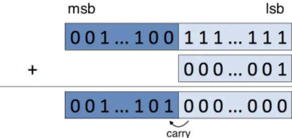
Figure 3: Addition with a carry digit in a large number with 2 limbs.
Figure 3 illustrates the addition of one to a limb that cannot represent the next integer
number. In this case study, a carry is generated and the limb is reset to zero. The overflow is detected if the second operand is greater than the result. In this case we add the carry result to the next more significative limb, and so on and so forth.
The MP module implements the addition algorithm (Algorithm2.1). In line 3, an
over-flow may occur, which in turn may generate a carry. Thus, the addition result cannot fit in the variable s. In this case there are three possibilities to overcome this situation:
• Use a machine instruction that gives the possible carry;
• Compute the module T, t = ai+bi−T. Then, to verify if the carry occurs, do the comparison t≤ai;
• Reserve a bit to check the carry occurrence, taking β≤T/2.
Algorithm 2.1Integer Addition, presented in [Brent and Zimmermann(2010)].
Require: A= ∑in=−01aiβi, B= ∑in=−01biβi, carry 0≤din ≤1 Ensure: C =∑ni=−01ciβi, 0≤d ≤1 1: d =din 2: for i =0; i<n−1 do 3: s= ai+bi+d 4: d=s div β 5: ci =s mod β 6: end for 7: return C, d
The subtraction algorithm is very similar to Algorithm2.1. The only difference is in line
3, that is stated as ’s= ai−bi+d’.
2.1.4 Multiplication
It is common to use algorithms that exchange some multiplications for additions, even if it brings some overhead associated.
In the multiplication, the choice of a particular algorithm is dependent on the input sizes and how fast a particular implementation is. Therefore, we implemented thresholds to determine which algorithm should be used to a certain situation. The thresholds are defined according to the performance of each algorithm. Several factors have an effect in the thresholds, i.e, the addition performance, where the the thresholds are as small as additions are faster. Figure4illustrates which is the best algorithm to multiply two numbers
of x and y limbs. This technique is called of squaring.
Most of the proposed algorithms work with operands of the same input-size. However, the multiplications are unbalanced in most real problems. There are two main strategies to face this problem:
• to split the operands into an equal number of limbs of unequal sizes.
Figure 4: The best algorithm to multiply two numbers of x and y limbs. bc is long multiplication, 22 is Karatsuba’s algorithm and 33, 32, 44 and 42 are Toom variants (from [Brent and Zimmermann(2010)]).
Long multiplication
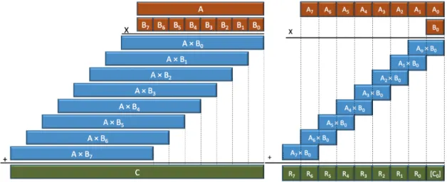
Several multiplication algorithms have been studied for decades. The long multiplication algorithm is the most used way to multiply two numbers by hand. It is the same algorithm taught in the elementary school. It is also known as schoolbook or basecase. Currently, it is the most efficient MP algorithm to multiply two operands with a small input size.
In line 3, the multiplication by βj is simple, because it only needs to shift the result by j limbs on the direction of the most significant bit. In this algorithm, the major work is done on the computation of A·bj, and on its accumulation to C. There are many techniques to optimize this step, but the basic one is to save all the multiplication results to an array. The accumulation of results on the array is very heavy to the pipeline, so to decrease its impact, the size of operand A has to be greater than the size of the operand B. For a graphic description of the algorithm, see Figures5and6.
Algorithm 2.2Long Multiplication, presented in [Brent and Zimmermann(2010)]. Require: A= ∑im=−01aiβi, B=∑ni=−01biβi Ensure: C =∑im=+0n−1ciβi, 0≤d≤1 1: A= A·b0 2: for j=0; j< n−1 do 3: C=C+βj(A·bj) 4: end for 5: return C
Grid method multiplication
Grid method multiplication, also known as box method, is other algorithm taught at ele-mentary school. It breaks the addition and multiplication of the long multiplication in two steps, which makes it less efficient than the long multiplication.
Booth’s multiplication
In 1950, Andrew Donald Booth invented a new multiplication algorithm [Booth (1951)].
Booth’s multiplication algorithm improves the multiplication performance, where the shift-ing operations are faster than addshift-ing operations. There is no gain of performance in mod-ern computers once shifting and adding operations take the same amount of time.
Figure 5: Long multiplication algorithm (from In-tel documentation).
Figure 6: Multiplication step (from Intel docu-mentation).
Gauss’ complex multiplication
The first fast multiplication algorithm was discovered in 1805 by Carl Friedrich Gauss [Knuth (1997)]. Gauss’s complex multiplication algorithm uses three multiplications and
mul-tiplications, which is not relevant for this dissertation. However, it was the beginning of the fast multiplication algorithms.
Karatsuba
The Divide and Conquer Algorithms (DCA) have a considerable value in MP arithmetic, i.e., Karatsuba and Toom-Cook algorithms [Knuth(1997),Mel(2007),Bodrato(2007)]. DCA
are algorithms based on multi-branched recursion. These algorithms work by recursively breaking down a problem into two or more sub-problems of the same type, until these become simple enough so no more breakdowns make sense. The solution of the original problem is given by the combination of the solution of all the sub-problems generated.
Algorithm 2.3Karatsuba’s Algorithm, presented in [Brent and Zimmermann(2010)].
Require: A= ∑im=−01aiβi, B=∑ni=−01biβi
Ensure: C =∑im=+0n−1ciβi, 0≤d≤1
1: if n<n0then returnBaseCaseMultiply(A, B) 2: end if 3: k = dn/2e 4: A0 = A mod βk 5: B0= B mod βk 6: A1 = A div βk 7: B1= B div βk 8: sA=sign(A0−A1) 9: sB = sign(B0−B1) 10: C0 =Karatsuba(A0, B0) 11: C1 =Karatsuba(A1, B1) 12: C2 =Karatsuba(|A0−A1|,|B0−B1|) 13: return C=C0+ (C0+C1−sAsBC2)βk+C2k 1
Karatsuba algorithm is one of the most important fast multiplication algorithms. Not only because of its good performance for small input sizes but because it opened the door to several algorithms and implementations. This algorithm is a divide and conquer algorithm for multiplication of integers discovered in 1960 by Anatoly Karatsuba. Since its publication several works have been done, such as parallel implementations [Kuechlin et al. (1991), Char et al.(1994)] and its analysis in distributed memory architectures [Cesari and Maeder
(1996)], generalizations [Weimerskirch and Paar(2006),Nursalman et al.(2014)] and FPGAs
[von zur Gathen and Shokrollahi(2006)]. Its goal is to reduce the number of multiplications
on a multiplication of two n-digit numbers to at most Θ(nlog23) ≈ Θ(n1.585) single-digit
multiplications. In practice, it reduces a multiplication of length n to three multiplications of length n/2, plus some overhead. Depending on the processor’s architecture, its optimal threshold can vary from 10 to 100 limbs.
There are many versions of the Karatsuba algorithm, where the addictive and subtractive versions are the most known. Despite the small difference between them, the subtractive version is more attractive since it avoids possible carries. Thus, it is not necessary to have carry verification step, which makes the subtractive version more efficient.
Algorithm 2.3 illustrates the subtractive Karatsuba version. The different between both
versions is stated as|A0−A1|and |B0−B1|instead of A0+A1 and B0+B1, at line 12. In lines 4-7, the operations mod and div are not executed in the implementation. It is only a mathematical way to indicate where the large number is split. Here, A0and B0have always the same number of limbs, but A1and B1 can deal with different sizes.
Toom-Cook k-way
Toom-Cook k-way algorithms also follow the divide and conquer strategy. Its general idea is to split the problem in k sub-problems in each iteration. This new low complexity algorithm was proposed by Andrei Toom in 1963 [Toom(1963)], and later Stephen Cook cleaned the
description [Stephen A. Cook (1969)]. The most known version is 3-way, also known as
’Toom-3’. In practice, it reduces a multiplication of length n to five multiplications of length n/3, plus some overhead. In the end it has a complexity ofΘ(nlog35) ≈Θ(n1.465). In general,
Toom-Cook k-way goal is to reduce the number of multiplications on a multiplication of two n-digit numbers to 2k−1 products of about n/k limbs, thus it complexity is Θ(nυ) where υ = loglog(2k(k−)1). An interesting fact is that the 2-way version is known as the Karatsuba
algorithm, where the Toom-Cook is its generalization. Toom-Cook algorithm is typically used for intermediate input-size multiplications, because of the overhead associated that makes it slower than Karatsuba and long multiplication algorithms.
Algorithm 2.4Toom-Cook 3-Way Algorithm, presented in [Brent and Zimmermann(2010)].
Require: A= ∑im=−01aiβi, B=∑ni=−01biβi, n1≥3 Ensure: C =∑mi=+0n−1ciβi
1: if n<n0then returnKaratsuba(A, B) 2: end if 3: write A=a0+a1x+a2x2, B=b0+b1x+b2x2 with x=βk 4: υ0= ToomCook3(a0, b0) 5: υ1= ToomCook3(a0+a1+a2, b0+b1+b2) 6: υ−1= ToomCook3(a0+a2−a1, b0+b2−b1) 7: υ2= ToomCook3(a0+2a1+4a2, b0+2b1+4b2) 8: υ∞ =ToomCook3(a2, b2) 9: t1 = (3υ0+2υ−1+υ2)/6−2υ∞ 10: t2 = (υ1+υ−1) 11: c0 =υ0, c1 =υ1−t1, c2=t2−υ0−υ∞, c3 =t1−t2, c4= υ∞
Algorithm2.4uses 5 evaluation points (0, 1,−1, 2,∞) and tries to optimize the evaluation
and interpolation expression. The division in line 9 and 10 needs to be exact. The division operation is a heavy operation, but as the dividend is a 6 it is possible to do the division by shifting the number, followed by a division by three.
FFT-based
Despite Karatsuba and Toom-Cook algorithms have a good performance in its sequential version, Fagin claimed that they are not good candidates for parallel implementations due to its divide and conquer strategy, which requires a lot of interprocess communication [Fagin(1992)]. He also claims that the FFT-based algorithms are more suitable in parallel
implementations, where several studies have been done [Jamieson et al. (1986), Johnsson et al. (1988)]. In addition to the inherit parallel properties, FFT-based algorithms are the
more suitable algorithms for input-sizes with thousands of digits. Currently, there are two main FFT-based algorithms used in MP integer arithmetic.
Sch ¨onhage–Strassen algorithm is a FFT-based algorithm that was developed in 1971 by Arnold Sch ¨onhage and Volker Strassen [Sch ¨onhage and Strassen (1971)]. Currently, it is
the most used FFT-based algorithm for large MP numbers, because of its low asymptotic complexityΘ(n·log(n) ·log(log(n))). In practice, it uses recursive FFTs in rings with 2n+1 elements. Until 2007, when the F ¨urer’s algorithm was published [F ¨urer (2007), Covanov and Thom´e(2015)], the Sch ¨onhage–Strassen was the algorithm with the lowest asymptotic
complexity. Anindya De was the first to purpose a similar approach that relies on modular arithmetic [De et al.(2008)]. In 2014, the asymptotic complexity of O(n·log(n) ·22log∗(n))
was achieved by David Harvey with a modification to F ¨urer’s algorithm [Harvey et al.
(2016)]. However, it only gets an advantage for considerable large MP numbers, which
makes it unpractical.
2.1.5 Division
The division is one of the most important algorithms to be optimized, because it uses to be one of the most heavy operations. A good strategy is to replace divisions by multiplications (e.g. precomputing the divisor’s inverse). Usually, MP division algorithms perform more multiplications than divisions. Thus, the multiplication algorithms, such as Karatsuba, have an important role in the division algorithms, since its performance has a direct impact. Therefore, it is important to optimize well the multiplication.
As multiplication, there are two types of division algorithms. Slow division algorithms obtain a limb of the final result at each iteration. On other hand, fast division algorithms start with an approximation of the final number and compute a more accurate number after each iteration, i.e., Newton–Raphson and Goldschmidt algorithms.
In all division algorithms the divisor must be normalized. A number is normalized when its most significant limb satisfies bn−1 ≥β/2.
Algorithm 2.5Long Division, presented in [Brent and Zimmermann(2010)].
Require: A= ∑in=+0m−1aiβi, B=∑ni=−01biβi, B normalized, m≥0 Ensure: Q =∑mi=−01qiβi, 0≤R< β 1: if A ≥βmB then qm =1 , A= A−βmB 2: else qm =0 3: end if 4: for i =m−1; i≥0 do 5: q∗ i = b(an+iβ+an+i−1/bn−1)c 6: qi =min(q∗ i, β−1) 7: A= A+qiβiB 8: while A<0 do 9: qi = qi−1 10: A= A+βiB 11: end while 12: end for 13: return Q, R= A Long division
The long division algorithm [Knuth(1997)], also known as schoolbook division, is the
stan-dard division algorithm taught in the elementary school. As the DCA, it breaks a large di-vision in a set of smaller problems, allowing the computation of large MP numbers. There are several variants of the long division such as the short division (used when the divisor is 1 limb size), and chunking method that is less efficient than the current long division al-gorithm introduced in 1600 by Henry Briggs. This alal-gorithm has an asymptotic complexity of O(n2).
Division by a limb
The single limb division is used when the divisor is represented with only one limb. It allows further optimizations. It can be both implemented with hardware division instructions or a multiplication by inverse [Moller and Granlund(2011)]. The choice of the method depends
on the hardware. For example, CPUs with low latency multipliers can perform the main operation much faster than a hardware divide instructions. However, due to the cost of calculating the inverse, it compensates for input-sizes larger than 4-5 limbs.
Exact division
The exact division algorithm is used when it is known that the remainder of certain division is zero. This knowledge allowed Jebelean to do some significant optimizations [Jebelean
(1993),Krandick and Jebelean(1996)]. This algorithm can be used within fast multiplication
algorithms, such as Karatsuba algorithm and Toom-Cook generalizations [Jebelean(1996)].
Algorithm 2.6Long division (binary version), from Wikipedia. Require: A= ∑in=+0m−1aiβi, B=∑ni=−01biβi, B normalized, m≥0 Ensure: Q =∑mi=−01qiβi, 0≤R< β 1: Q=0 2: R=0 3: b=getNumberOfBits(A) 4: for i =b−1; i≥0 do 5: R= R<<1 6: R(0) =N(i) 7: if R≥B then 8: R=R−B 9: Q(i) =1 10: end if 11: end for 12: return Q, R
Usually, if the divisor is larger than a certain threshold the division is done with a divide and conquer algorithm [Burnikel et al.(1998),Moenck and Borodin(1972),Jebelean(1997), Hart (2015)]. Unlike the long division that determines a limb of the final result at each
iteration, the divide and conquer division tries to get several limbs at once. It divides the original MP number in smaller MP numbers. Thus, it is possible to speedup the main division by using fast multiplication algorithms in smaller operands.
2.1.6 Newton’s method
Newton’s method, also known as Newton–Raphson method, is a fast division algorithm with the best asymptotic complexity [Schulte et al.(1994)]. It was created by Isac Newton
and Joseph Raphson. Newton’s method is widely used in number theory to solve several problems, such as the computation of roots. This method finds a reciprocal of the divisor and multiply it by the dividend. This, it successively finds better approximations of the final quotient.
Barret’s division
Barret’s division is a reduction algorithm created by Paul Barrett in 1986 [Barrett (1987)]
to speedup the RSA encryption algorithm on an ’off-the-shelf’ digital signal processing chip. It is designed to replace division by multiplications. Its first version just uses a single limb. However, this version is not able to perform MP divisions. Therefore, Barret propose a second version of his algorithm that approximates to the single limb implementation [Menezes et al.(1996)].
2.1.7 Hensel’s division
Classical division algorithms usually cancel the most significant part of the MP number. However, Hensel’s division algorithm cancels the least significant part of the number. The big difference of this strategy is that it is not necessary a correction step, since carries go in the opposite direction of the classical algorithms. There are cases, where only the remainder is desirable. In that cases this algorithm is known as Montgomery reduction [Knezevic et al.
(2010)].
With so many algorithms available it is hard to select which one is the best for certain operation. In 2003, Karl Hasselstr ¨om compared some of the most prominent MP division algorithms for several input-sizes [Hasselstr ¨om(2003)].
Algorithm 2.7Division By a Limb, presented in [Brent and Zimmermann(2010)].
Require: A= ∑im=−01aiβi, 0≤c< β Ensure: Q =∑mi=−01qiβi, 0≤b<1 1: d =1/c mod β 2: b=0 3: for i =0; i<n−1 do 4: if b≤ ai then 5: x= ai−b 6: b 0 =0 7: else 8: x= ai−b+β 9: b 0 =1 10: end if 11: qi =dx mod β 12: b 00 = (qic−x)/β 13: b= b 0 +b00 14: end for 15: return∑n−1 0 qiβi, b
2.2 l at t i c e b a s i s r e d u c t i o n
Lattice basis reduction is a subgroup of problems in lattices. As mentioned before, the lattice basis reduction goal is to transform a given basis B of a lattice L into a closer to orthogonal and shorter basis such thatLremains the same. The quality of a basis depends on the shortness and orthogonality of the basis vectors and other factores [Xu (2013)]. In
order to reach that, it is possible to use the following operations:
• Swap two vectors of the basis. The swapping changes only the order of vectors in the basis it is trivial because L is not changed;
• Replace bj by−bj. It is trivial becauseLremains the same;
• Subtracting or adding to a vector bj a combination of other vectors of the basis B. The lattice is not changed because when it is used an arbitrary vector that belongs to the lattice L, it is achieved another vector that belongs toL. Mathematically, if a vector is replaced by bj ← bj+∑i6=jzibi, a new basis is obtained that will generate the same lattice L.
Figure 7: Lattice reduction in two dimensions: the black vectors are the given basis for the lattice, the red vectors are the reduced basis (from Wikipedia).
Lattice basis reduction is used to achieve the shortest vector of a basis when its rank is small. To higher ranks there is not known any algorithm to solve the SVP in polynomial time, but some lattice reduction algorithms can find a nearly short vector in polynomial time [Lenstra et al. (1982a)], which is enough to some applications. The figure 7shows a
basis reduction example, where vi is the vector of a basis B, and ui are the resultant vectors of the lattice basis reduction.
Finding a good reduced basis has proved helpful in many fields of computer science and mathematics, particularly in cryptology. A good example is the execution time of the SVP-solvers, where they took less time to finish in good quality basis.
2.2.1 Basic Concepts
This section contains some concepts that are important to easily understand about lattices and its inherit problems.
Determinant of a lattice
An interesting feature of a latticeLis its determinant (detL), a relevant numerical invariant. Thus, two different basis with the same latticeLwill have the same determinant because it does not depend on the choice of a basis B. Geometrically, the determinant is the volume of the parallelepiped spanned by the basis.
In a full rank basis, where the number of basis vector is equal to the spanned dimen-sion, the determinant of basis B is the volume of the parallelepiped spanned by its vectors. Besides, if the number of vectors is less than the dimension of the underlying space, then volume is
q
det(BTB). In resume for a full rank lattice, we have: det(L) =det(B) =
q
det(BTB) (2)
Gram Matrix
The Gram Matrix of a set of vectors B is a square matrix composed of all possible inner product entries (Equation3). This matrix is symmetric which means that G = GT. It has
important applications, such as the computation of linear independences, where a set of vectors is linearly independent if its determinant is different from zero. It will be widely used in a lattice reduction algorithm that will be presented ahead.
Gij = hBi, Bji (3)
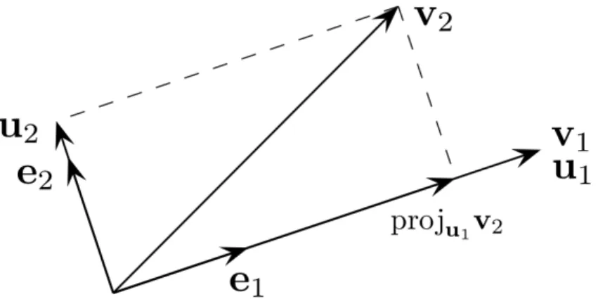
Gram-Schmidt coefficients
Gram-Schmidt (GS) orthogonalization is a process to orthogonalize a set of vectors, i.e., a lattice basis. It computes an orthogonal basis B∗for the same vector space, where all vectors are orthogonal to all previous basis vectors. During the GS process the GS coefficients
and norms are computed. For advantage of some lattice reduction algorithms, the GS orthogonalization is computed iteratively by:
b∗i =bi− j<i
∑
j=0
µi,jb∗j, where µi,j =
hbi, b∗ji
hb∗j, b∗ji (4)
The GS coefficients (µ) and its norm vectors are widely used in some lattice reduction algorithms, since it helps to get a more orthogonal basis. Notice that the orthogonal basis cannot belong to the lattice L. Figure8 illustrates an example of the first two steps of the
GS orthogonalization, where ei are normalized vectors.
Figure 8: The first two steps of the Gram–Schmidt orthogonalization (from Wikipedia).
Lattice basis type
Lattice reduction algorithms can have different behaviours depending on the type of input basis. Therefore, it is important to study the behaviour of different algorithms in different types of basis.
There are ways to generate lattices that converge to an uniform distribution, accordingly to the Haar measure30
, when the integer parameters grow to infinity. Goldstein and Mayer (GM) are an example of a basis that converge to an uniform distribution [Goldstein and Mayer (2003)]. This type of bases follows the next steps to generate a basis of dimension
n (i) choose a large prime integer p, (ii) choose randomly n−1 numbers (xi) where xi are integers in the range 0≤ xi < p. Figure 9illustrates some examples of GM matrices.
We also performed tests in Ajtai-type bases [Ajtai(1996)]. Ajtai introduces similar bases
[Ajtai (2003)] to prove a lower-bound on the quality of Schnorr’s block-type algorithms
[Schnorr(1987)]. These bases are upper-triangular matrices where (i) it is chosen a random
parameter a, (ii) bi,i = b2(2n−i+1)
a
e, (iii) the bi,j0 s where i> j are independent, randomly and uniformly selected in Z∩ [−bj,j
2 , bj,j
2 ]. The advantage of chose bi,i = b2
(2n−i+1)a
e is that the kb∗ik’s decrease quickly, thus the basis is far from being reduced.
GM bases have to use MP arithmetic. Besides, Ajtai-type bases can be represented in primitive data types.
Figure 9: Examples of GM matrices.
2.2.2 Lenstra–Lenstra–Lov´asz
The Lenstra–Lenstra–Lov´asz (LLL) was the first prominent lattice basis reduction algorithm to be introduced. The LLL is a polynomial time algorithm invented by Arjen Lenstra, Hendrik Lenstra and L´aszl ´o Lov´asz in 1982 [Lenstra et al. (1982b)]. Currently, the LLL
algorithm has been successfully implemented, due to the Lov´asz condition that controls swapping operation between basis vectors. Therefore, all of the following works are mainly focused on (i) understanding statistical mean running behaviour and average complexity of the LLL algorithm [Nguyen and Stehl´e(2006)] and (ii) improving the efficiency and stability
of the LLL algorithm [Artur Mariano and Bischof(2016)]. An interesting fact is that many
simulations and theoretical analysis confirm that the LLL algorithm performs much better in practice than the worst case bound of complexity.
LLL algorithm
The LLL algorithm is split into two main components. The first one aims to make the basis more orthogonal as possible with the Gram-Schmidt coefficients by computing a size-reduction of the vector bk. It is a size-reduced basis when|µij| ≤ 12, where(1 ≤ j<i≤ n) inRn. Usually the basis is size-reduced, but when|µij| > 12 it replaces bi with(bi− dµijcbj). The size-reduction component is described in Algorithm2.8between lines 4 and 9.
In the second component, it implements the Lov´asz swapping condition to make the reduced vectors as short as possible. The Lov´asz condition is denoted by:
δkb∗ik2≤ kb∗i+1+µ(i+1)ib∗ik2 (5) where δ=3/4. A robust swapping condition implies using a larger value for the control parameter δ in the condition, which can be between 0.95 and 0.999. If the swapping is necessary, the vectors bi and bi+1 will exchange themselves and then set the current stage of (i+1)back to i.
Since LLL algorithm was proposed, several works have been done. However, only two major improvements were done. First, a very efficient floating-point version was proposed by Schnorr [Schnorr and Euchner (1994)], allowing to solve some exact problems more
efficiently. Avoiding MP arithmetic and using primitive floating-point data types results in faster computations and in a minor number of swaps. Later, other floating-point versions appear with further optimizations [Nguˆen and Stehl´e(2005)] that reduced the asymptotic
complexity. Despite this optimization speeds up the LLL algorithm, it needs to be used with caution since it introduces floating-point errors.
Algorithm 2.8LLL algorithm, presented in [Nguyen and Stehl´e(2006)].
Require: A basis (b1, ..., bn)and δ∈ (14, 1) Ensure: A LLL−reduced basis
1: Compute Gram-Schmidt coefficients and norms
2: k =2 3: while k≤n do 4: for i=k−1 to i=1 do 5: bk =bk− dµk,icbi 6: for j=1 to i do 7: µk,j =µk,j− dµk,icµi,j 8: end for 9: end for 10: k0 =k 11: while k>2 and δck−1 >ck0+∑k 0−1 i=k−1µ2k0,ici do 12: k=k−1 13: end while
14: Insert bk0 right be f ore bk
15: k=k+1
16: end while 17: return B
The original LLL algorithm runs in polynomial time but it is just capable of generates a basis with medium quality. It led Schnorr and Euchner to propose the second major improvement. They introduced a LLL algorithm with a deep insertion technique. [Schnorr and Euchner(1994)], which allows to find shorter basis vectors, resulting in better reduced
bases. In practice, it replaces the swapping step by a deep insertion. As well as the original LLL algorithm, this implementation make use of the Gram-Schmidt coefficients to make the basis as orthogonal as possible, but the Lov´asz condition is overwritten by a ’deep insertion’ to achieve a basis with shorter vectors. Thus, the algorithm computes the following stronger condition: δkb∗ik2≤ kb∗k + k−1
∑
j=i µljb∗jk2 (6)where δ = 3/4, until it is true or i < k. If the condition is true the algorithm will insert bk right before bi. Schnorr and Euchner also proposed using a bigger value of δ=0.99.
At first, the complexity of the LLL algorithm with deep insertions was super polynomial, with examples showing that its practical running time is longer by a few times than the original LLL algorithm, but Gama and Nguyen [Gama and Nguyen (2008)] reported that
the Schnorr version has super exponential complexity.
2.2.3 Hermite-Korkine-Zolotarev
The Hermite-Korkine-Zolotarev (HKZ) is a lattice-reduction algorithm that achieves re-duced basis with better quality. Its vectors are more orthogonal and shorter than the previ-ous LLL algorithms, but it requires more computation time to converge [Hanrot and Stehl´e
(2008)].
A basis B of a latticeL, is HKZ-reduced if its first vector reaches the minimum ofLand if orthogonally projected to b1the other vectors bi’s are themselves HKZ-reduced.
2.2.4 Block-Korkine-Zolotarev
Schnorr proposed several works during its career. In 1994, he introduces a new lattice ba-sis reduction algorithm [Schnorr and Euchner(1994)]. The Block-Korkine-Zolotarev (BKZ)
combines the quality basis output of the HKZ with the good execution times of LLL. It combines a lattice basis reduction algorithm with an SVP-solver, the LLL algorithm and an enumeration algorithm respectively. In BKZ, the lattice reduction algorithm and the enu-meration algorithm are dependents on each other, and the enuenu-meration algorithm operates as a function of the main algorithm.
The BKZ have an extra entry parameter ω that defines the window size. The window corresponds to the block of basis vectors where the enumeration algorithm executes. A bigger block size results in a more reduced basis. However, it is necessary some caution on choosing the window size since the running time increase significantly. It happens because the enumeration algorithm is super-exponential, (2O(ω2)). The BKZ with ω = 20
is very practical, but when the block size increases to ω ≥ 25, its running time increases significantly, which makes any high block size impracticable. This was the Achilles heel of the original BKZ, denying the possibility to operate with bigger blocks size.
The BKZ algorithm starts by calling the LLL algorithm to obtain a LLL-reduced basis and then it behaves like a sliding window over the basis, that will call successively an enumeration function, that returns the shortest vector found in the projected basis. Then, if a shorter vector is found, it is added to the current basis and the LLL algorithm is called again to remove the generated dependency.
Algorithm 2.9BKZ algorithm, presented in [Chen and Nguyen(2011)].
Require: A basis(b1, ..., bn), its GramSchmidt orthogonalization, i.e., µ and ci, a block size ω ≥ 2, and δ∈ (1
4, 1)
Ensure: A BKZ ω−reduced basis
1: z =j=0 2: LLL(B, δ) 3: while z<n−1 do 4: j= (j mod(n−1)) +1 5: k=min(j+ω−1, n) 6: h=min(k+1, n) 7: v=ENUM(µ, c) 8: if v6= (1, 0, ..., 0)then 9: z=0 10: LLL((b1, ...,∑k i=jvibi, bj, ..., bh), δ) 11: else 12: z=z+1 13: LLL((b1, ..., bh), δ) 14: end if 15: end while 16: return B BKZ 2.0
Lately the BKZ 2.0 was presented by Chen and Nguyen [Chen and Nguyen (2011)], that
made the first experiments in higher blocks size, ω ≥ 40. The BKZ 2.0 can be considered an updated BKZ which came with four improvements:
• An early-abort;
• A sound pruning enumeration; • Preprocessing of local blocks; • Optimizing the enumeration radius.
The first improvement is simply an early-abort and was based on a theoretical result of Harrot [Hanrot et al. (2011a)]. This improvement results on the addition of a parameter
that specifies how many iterations should be performed. The improvement delivers an exponential speed up over BKZ over call with higher blocks size.
The other three improvements are related with the enumeration subroutine. The main modification consists in the incorporation of the sound pruning technique developed by Gama, Nguyen and Regev [Gama et al.(2010)]. The sound pruning uses specific bounding
functions to discard some branches where the probability of to find a shorter vector is too small.
The cost of the enumeration subroutine is correlated with the quality of the reduced basis. Unfortunately, the BKZ only guarantees an LLL-reduced basis, which can be too expensive with higher blocks size. Thus, the BKZ 2.0 guarantee a stronger lattice reduction algorithm by preprocessing local blocks.
When the enumeration subroutine starts, the initial radius R used to be initialized as R = kb∗jk. Unfortunately, this radius could be far from the norm of the shortest vector, what will take more computation than if a nearby radius was defined. However, there is no theoretical proof of which size must be the initial radius. Thus, the radius approximation is based in the Gaussian Heuristic (GH), that provides a good estimate for the norm of the shortest vector of the lattice L. The GH is denoted by:
GH(L) =F( n 2+1)
1
n ×det(L)1n (7)
where det(L)is the determinant of the latticeL, and:
F(n) = (n−1)! (8)
2.2.5 Qiao’s Jacobi method
The Jacobi method proposed by Sanheng Qiao in 2012 is a recent algorithm for lattice basis reduction that claims to reduce a lattice basis with better orthogonality in less time than LLL algorithm [Qiao(2012)].
The Jacobi method is a very attractive algorithm because it is inherently parallel, due to matrix computations [Golub and Van Loan(1996)] that are the majority of the algorithm.
Thus, there is a great chance to exploit parallel microarchitectures and improve its perfor-mance.
Lagrange’s algorithm computes a reduced basis in a two-dimensional lattice, where S. Qiao found an algorithm that uses this principle, and given a lattice basis A, it gets an unimodular matrix Z of the same size, where AZ forms a reduced basis. The algorithm consists in applying the two-dimensional Lagrange’s algorithm to all possible pair of vec-tors in original basis A. For a detailed description see the original paper [Qiao(2012)].
The Jacobi method output is said to be Lagrange-reduced (L-reduced). Thus, the basis A is conspired L-reduced if:
kaik ≤ kajk (9)
|aTiaj| ≤ kaik2
2 (10)
![Figure 4 : The best algorithm to multiply two numbers of x and y limbs. bc is long multiplication, 22 is Karatsuba’s algorithm and 33 , 32 , 44 and 42 are Toom variants (from [Brent and Zimmermann ( 2010 )]).](https://thumb-eu.123doks.com/thumbv2/123dok_br/17560177.817322/22.892.149.806.198.704/figure-algorithm-multiply-multiplication-karatsuba-algorithm-variants-zimmermann.webp)

![Figure 10 : Chess tournament with n = 8 (from [Jeremic and Qiao ( 2014 )]).](https://thumb-eu.123doks.com/thumbv2/123dok_br/17560177.817322/38.892.148.805.194.480/figure-chess-tournament-n-jeremic-qiao.webp)