DEMAND FOR TRUCKS IN BRAZIL: AN ECONOMETRIC APPROACH ABSTRACT
The demand for trucks in Brazil has historically been an unusual choice for econometric analysis, resulting in a scarcity of studies on this subject, inconsistent with the economic relevance of road freight transport and its historical dominance over any other means of transport in the country. This paper addresses the demand for trucks in Brazil, making extensive use of secondary data in multiple linear regression models. Besides the choice of the subject itself, it innovates by including expectational variables to the analysis. In comparison to the surveyed studies on passenger car demand, further improvements were undertaken, as the split of GDP in sectors (agriculture, industry and services), the use of lagged variables, and a nineteen years long timeframe (from 1996 to 2015).
The results deepen the knowledge about the truck market behaviour and allow an improvement of the quality of decision making in the truck industry.
Keywords
Truck Market, Truck Demand in Brazil, Truck Sales, Commercial Cargo Vehicles Demand, Automotive Industry, Automotive Market Analysis, Multiple Linear Regression, Econometric Model, Expectational Variables, Sector-sensitive Demand for Transportation
INTRODUCTION
Of all cargo hauled in Brazil, 61% is transported by trucks, 21% through railways and only 14% along waterways (DNIT - National Department of Transport Infrastructure, 2015). Around 1.8 million trucks 1 (SINDIPEÇAS - Brazilian Association of Automotive Components Manufacturers, 2015) operate along 1.6 million kilometres of roads (CNT - National Confederation of Transport, 2015), connecting up to 5,561 municipalities, to supply its 8.5 million square kilometres territory (IBGE - Brazilian Institute of Geography and Statistics, 2015). Eleven companies - nine local manufacturers and two importers - compete in the Brazilian domestic truck market (FIPE - Institute of Economic Research Foundation, 2015). Over 50% of this market is split between the two major players, resulting in a moderately concentrated oligopoly, with a HHI (Herfindahl-Hirschman Index) of 0.19.
This paper models domestic truck demand in Brazil using multiple linear regressions with data from 1996 to 2015. It uses variables traditionally adopted in vehicle demand analyses such as price, Gross Domestic Product (GDP) and credit, adds expectational variables and also uses a supply side decomposition of GDP to shed light in different transport intensity of different GDP components (e.g. agriculture requires much more cargo transportation than services). The fundamental question addressed is: what is associated with increases or decreases of truck sales in Brazil? This paper also takes into account potential structural breaks since 1996. Several econometric tests assure the statistical robustness of the model. In addition to this section, this work is structured as follows: (2) Literature Review of previous studies on vehicular demand (3) Data, Variables and Methodology detailing variables; (4) Results and Analysis discussing the
1 Truck: automotive vehicle intended to transport cargo or tract another vehicle, exceeding 3.5 tons of total gross weight.
models and corresponding econometric tests; and (5) Conclusions containing a discussion of the results, their relevance, contributions, and opportunities for future research.
LITERATURE REVIEW
The reviewed literature includes studies conducted in Brazil, United States, Canada, United Kingdom, and New Zealand (limited to Portuguese and English language sources) and shows that the focus of vehicular demand studies, both in national and international settings, is directed to passenger cars, not specifically addressing trucks and other classes of terrestrial automotive vehicles. Some studies of the international truck market adopt different approaches, modelling disaggregated demand (Dorward et al. 1983) or analysing industry structure (Buckley and Westbrook, 1991).
Concerning econometric modelling, some automotive models have price as dependent variable (Angelo and Favero, 2003; Bajic, 1988; Cowling and Cubbin, 1971; Gual, 1993; Hoffer et al., 1971; Turnovsry, 1966), others, vehicular quantity demanded.
As for methodology, the approaches are divided in univariate time series (Davies Junior, 2011; Lourenço and Nascimento, 2012) and regression analysis. The multiple linear regression models, on their side, are divided in market share (Berry et al., 2004; Dorward et al., 1983; Fiuza, 2002; Hess, 1977; Irvine, 1983; Morais and Portugal, 2005; Schiraldi, 2011; Tishler, 1982) and total demand analyses (Baumgarten Júnior, 1972; Moraes and Silveira, 2005; De Negri, 1998; Dyckman, 1965; Fauth et al., 2011; Gabriel, 2013; Hymans et al., 1970; Rippe and Feldman, 1976; Roos and Von Szeliski, 1939; Vianna, 1988; Villela, 2014; Wilton, 1972; Witt and Johnson, 1986; Wolff, 1938).
Linear and translogarithmic models are both common. Lagged models are predominant amongst international studies, while unlagged ones are more common in Brazilian analyses. Concerning
the choice of variables, a pattern emerges: despite different proxies in each study, price and income variables are omnipresent. On the other hand, variables for credit are adopted more often in Brazilian models (restriction to credit availability is, possibly, not a relevant characteristic in the international environments analysed) while fleet size (as a proxy for market maturity) is more frequent in international studies. Market size is also a relevant variable in the literature. Other variables were also employed to address market peculiarities or specificities of each study, but no recurrent pattern emerged.
In Brazil, Baumgarten (1972) was the pioneer on vehicular demand analysis, modelling the Brazilian passenger car market using lagged variables. Vianna (1988) differs from international analyses in considering credit (total volume of credit in the economy, average grace period, and percentage of credit transactions directed to vehicle financing) as a relevant variable in Brazilian automotive market. The same choice of variable (price, income and credit) as in Vianna (1988) is also found in De Negri (1998), Gabriel (2013) and Moraes and Silveira (2005). Fauth et al. (2011) and Gonçalves (2016) differ from the previous authors in one important way: trucks are included in their demand analysis. Fauth et al. (2011) split the analysis among three classes of vehicles: cars, trucks and buses. The model contains usual variables as price, income and credit but also the price of substitute products. Dummy variables are added to account for the effect of disturbances caused by the exchange rate and presidential elections. Villela (2014) detects unit roots, adopting cointegration analysis to deal with the problem. The usual variables (price, credit and income) are used without lags and the model is split to account for structural breaks.
DATA, VARIABLES AND METHODOLOGY
The database is composed of secondary data from government sources as IBGE, DENATRAN (National Department of Transportation) and BNDES (National Bank for Economic and Social
Development), research institutes as FGV (Getulio Vargas Foundation), FEA (School of Economics, Business and Accounting of the University of São Paulo), IPEA(Institute of Applied Economic Research) and IBRE (Brazilian Institute of Economics), and associations and federations as ANFAVEA (National Association of Motor Vehicle Manufacturers) and FENABRAVE (Automotive Vehicles Distribution National Federation), and is available from the corresponding author.
Information deemed relevant are unavailable, especially the fleet size (for all kinds of vehicles, including trucks), as acknowledged in the National Emissions Inventory from the Ministry of Environment (Minc, 2013): “(…) The estimation of the national fleet was still based on theoretical scrap curves applied to the licensing and sale of new vehicles, with the recommendation that they should be calibrated and updated by comparing registered fleet data with vehicle data licensed annually by DETRAN in the states, seeking better adherence to actual circulating fleet”. The available data on fleet size from DETRAN (State Department of Transportation), DENATRAN and ANTT (National Agency of Terrestrial Transportation) were not considered because they are very distorted. The vehicles’ scrapping rate and fleet average age were also ignored for the same reason.
Domestic truck sales are seasonal. Data are intentionally not seasonally-adjusted. Nominal monetary variables (as currency or indexes) are expressed in real terms, adjusted for inflation by the IGP-DI (General Price Index-Internal Availability - a comprehensive Brazilian price index provided by Fundação Getulio Vargas).
The dependent variable for the domestic truck demand in Brazil (TruckDemand) is based on monthly sales data, available from ANFAVEA since January 1957. These data refer to the amount of monthly licensed vehicles in Brazil (sales before 2002 are wholesale truck transactions). Sales figures include imported vehicles, and exclude exported ones, capturing
domestic apparent demand. The time series TruckDemand runs from January 1996 to December 2015.
The variable for truck prices (PriceIndex) stands for the average truck acquisition price. It is an index based on the arithmetic average of the prices of the most representative vehicle models (according to each manufacturer’s criteria). It excludes value-added taxes (such as ICMS - Tax on Circulation of Goods and Transportation and Communication Services) but includes IPI (Tax on Processed/Manufactured Goods) in the series prior to 2010, while excludes both taxes after 2010 (IBRE, 2015) (no discontinuity was observed on price curve concatenation). The price proxy results from several series concatenations. The first time series, from 1969 to 2008, is a subseries of a broader producer price index(IPA-DI specific for trucks). From 2008 to 2015, two time series (provided by IBRE, upon a specific request) are merged: IPA-EP-DI, referring to monthly sales of tractor units, and IPA-EP-DI, referring to non-tractor units. A weighted average of these two phased series based on sales volumes of both categories (Environment Ministry - Minc, 2013) was the criterion for the merge. The concatenation of the first (1969-2008) and second (2008-2015) periods presents less than 0.1% discrepancy. The resulting series is rebased for 2015Q4 (the procedures to obtain this variable are available from the corresponding author). Agriculture, Industry and Services present different demands for transportation per monetary unit of respective contributions to GDP. To account for the three, the model splits the GDP in three components: GDPAgriculture, GDPIndustry and GDPServices referring to the GDPs from primary, secondary and tertiary sectors respectively. It is a departure from previous literature that considers only total GDP. All GDP data are adjusted for inflation but (intentionally) not for seasonality, and measured in average 2010 BRL millions.
Earmarked credit for truck acquisition (CreditGranted) is based on a time series provided by BNDES. Amounts are restated for 2015Q4 (BRL Millions) using IGP-DI. BNDES is the main
source of credit for truck acquisition (ANEF - National Association of Auto Industry Financing Companies - ANEF, 2016), leading to the use of earmarked credit granted by BNDES as a proxy for the volume of credit granted by all financing sources.
PurchasingPower is the variable for total labour income (IBGE, 2015).
GDP forecasts are from Banco Central do Brasil (Brazil Central Bank). The variable GDPForecast1 refers to the quarterly released expected GPD growth rate for the following year. Industry confidence level (IndConfidence) measures the expectations for Brazilian economy performance. Data are based on ISA (Current Situation Index), not seasonally-adjusted (The industry confidence index - ICI - is based on manufacturing industry survey conducted by IBRE and is the arithmetic average of the current situation index - ISA - and the expectations index - IE). It is worth emphasising that expectational variables were never used before in automotive demand modelling in Brazil, however, regular macroeconomic expectation surveys became available only after 2000. A proxy for buyer’s expectations was then chosen among the information available to the buyer from 1996 to 2000. IBOVESPA (Bovespa Index is a total return market-cap weighted performance index for stocks traded in B3 São Paulo Stock, Mercantile Futures Exchange) is adopted for this purpose when IndConfidence and GDPForecast1 were not available.
Table 1 shows the complete list of variables
================== Insert Table 1 about here ==================
A Two-Model Approach
This econometric model is a multiple linear regression based on non-seasonally-adjusted quarterly data, as previously detailed.
= + + + ⋯ + + ⋯ + + (1) Two issues deserve preliminary attention.
The first issue is non-stationarity. Brazilian truck sales present historical growing trend and are, consequently, a non-stationary process. Thus, when the dependent variable (TruckDemand) is tested for ADF(Augmented Dickey–Fuller test), unit roots are detected. This result automatically leads to problems for any set of independent variables chosen, since it renders impossible to construct a statistically robust multiple linear regression model using the time series of truck sales in Brazil as a dependent variable.
There are some alternatives to deal with the problem and proceed with the analysis, such as ECM or cointegration analysis. Here, the adopted approach was to take the first difference, the simplest acceptable way to deal with existence of unit roots, of the time series (Verbeek, 2004).
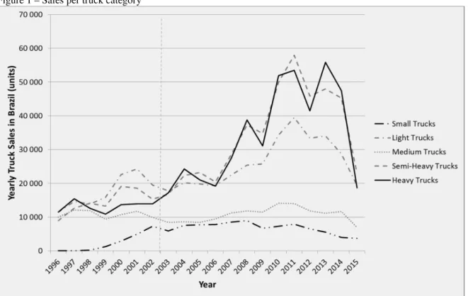
The second issue is a potential structural break. Truck sales have changed since 2003, and the previous balanced distribution among the five categories of trucks (small, light, medium, semi-heavy and semi-heavy) was replaced by a dominance of semi-semi-heavy and semi-heavy trucks (Figure 1Figure 1). At the same time (2003 was also the beginning of a presidential term), the maximum allowable loading for trucks in Brazil was considerably increased2.
================== Insert Figure 1 about here ==================
These events raise a reasonable question about the occurrence of a structural break around 2003. However, the statistical answer to this question requires a sufficiently long regression containing the year 2003 (Wooldridge, 2006). The unavailability of some time series in the required time
2In 1998, the first exceptions to the maximum allowed load of 45 tons were enacted (up to 74 ton for trucks with a special authorization). In 2006, new transport compositions, as Bitrem (two trailers per truck), were subjected to explicit regulation and the maximum load (with no special authorization required) was increased to 57 ton.
interval renders impossible a structural break test. As a consequence, the analysis was split in two models: before and after 2003. These periods include: F. H. Cardoso first presidential term (1995-1998), and his second term (1999-2002), Lula da Silva first (2003-2006), and second term (2007-2010), D. Roussef first term (2011-2014) and part of her second term (inauguration on January 1st, 2015). Analysis starts in 1996, and not in 1995 as would be desirable, due to data unavailability.
For both models time lags were determined through a stepwise process.
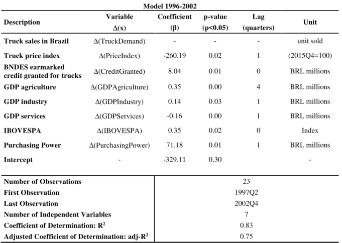
RESULTS AND ANALYSIS Model 1996 - 2002
Table 2 presents the results of the 1996-2002 model:
================== Insert Table 2 about here ==================
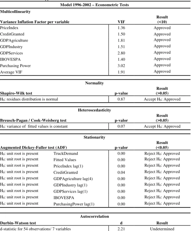
Table 3Table 3 shows the results of econometric tests for the 1996-2002 model.
================== Insert Table 3 about here ==================
Multicollinearity, non-normality or heteroscedasticity problems were not detected. Presence of unit roots was not confirmed at a confidence level of 95%. Autocorrelation test was inconclusive and this indetermination was taken as acceptable.
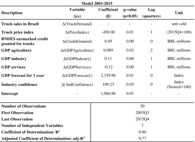
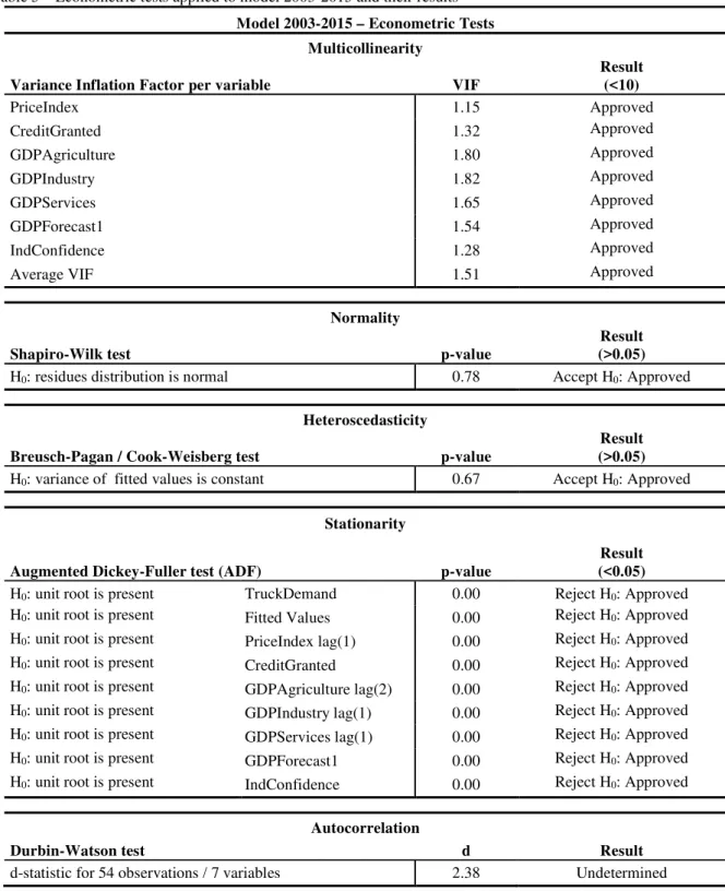
Model 2003 - 2015
Expectation surveys on macroeconomic performance became available in this period, replacing IBOVESPA in the model. Results are shown on Table 4Table 4.
================== Insert Table 4 about here ==================
Table 5Table 5 displays the econometric tests performed to model 2003-2015 and their results. ==================
Insert Table 5 about here ==================
Once again, the model passes all relevant tests. Multicollinearity or heteroscedasticity were not detected, as in the 1996-2002 model. Problems related to normality or stationarity were not detected as well. Results from autocorrelation test were not conclusive, and were taken as acceptable as in the 1996-2002 model.
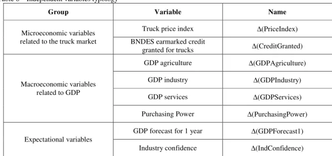
In model 2003-2015, it is possible to discern three sets of variables: microeconomic ones related to truck market, macroeconomic variables related to GDP and total labour income, and expectational variables of macroeconomic performance. They are described on Table 6Table 6. ==================
Insert Table 6 about here ==================
A Rough Comparison between Models
The adjusted coefficients of determination (adj-R2) are 0.77 and 0.75, for the first and second models respectively.
The expectational variables contain the main differences between models 1996-2002 and 2003-2015 and the different availabilities of these variables along the relevant time ranges (as IBOVESPA, used in model 2003-2015, and ISA, used in model 1996-2002) prevent direct comparison between the two models.
However, the similarity between them leaves room for some considerations. The main characteristics of each model are summarised on Table7Table7.
================== Insert Table7 about here ==================
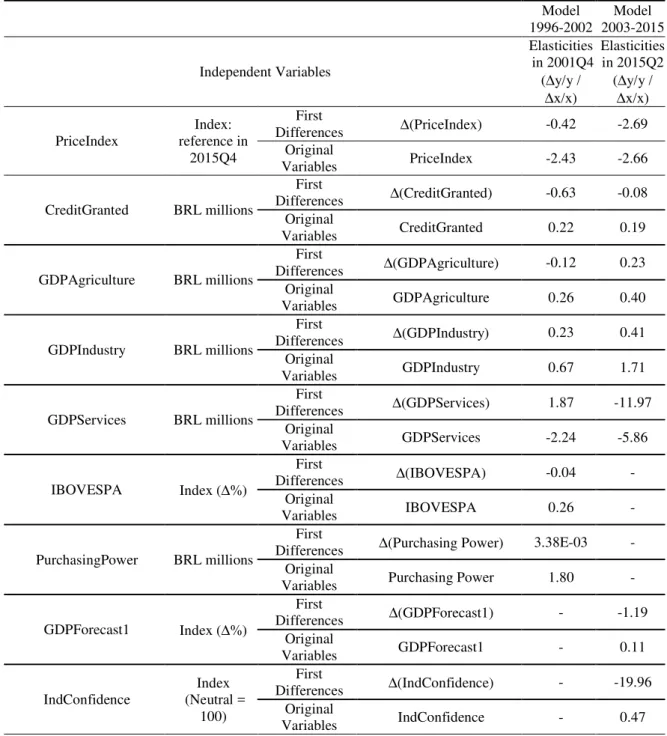
Most of the variables common to both models present the same lag. The exception is the agriculture GDP. Its lag was reduced from 4 to 2 quarters from the first to the second model. An Appendix displays elasticities of both models calculated for some specific dates: 2001Q4 and 2015Q2
CONCLUSIONS
This study differs from others found in the literature in several aspects.
A specific model for truck demand helps to fulfil an important gap in Brazilian automotive studies. As seen in the literature review, it distinguishes this paper from most of other vehicular demand analysis, concerned mainly with passenger cars.
There are three groups of variables: (1) microeconomic variables specific to the truck market; (2) macroeconomic variables; and (3) expectational variables.
Thus, the model not only makes the usual choice of variables, as GDP, but goes further and accounts for the effects from each sector separately: agriculture, industry and services. It includes
variables related to buyer’s confidence, absent in previous studies of the Brazilian automotive market.
The time frame of this analysis - spanning almost two decades - is not found in the previous literature. It makes use of lagged variables, long ignored in automotive demand models in Brazil. Buyer’s reaction to price variations is lagged. The lag of one quarter in relation to prices seems to indicate that the total time between price change and purchase (including dissemination of information, decision making and purchasing procedures) is longer than three months. However, buyer’s reaction to credit changes occurs within the same quarter.
GDP sector coefficients are similar (in module) but, it does not mean an equivalent importance of all three sectors on demand, given the considerable difference in GDP share among agriculture, industry and services. Agricultural GDP presents longer lag than the two others. Service GDP has a negative effect on truck sales, unlike the two others. This means that amongst all the possible influences from services (rise on available income, low demand for cargo transport, increase on economic activities and impact on contracted freights), the net effect is negative for truck sales. This is not trivial for the future behaviour of truck demand, since services actually constitute 75% of the Brazilian GDP and have been increasing their relative share.
The total labour income improves the quality (higher adj-R2) of the model 1996-2002, but is not relevant for model 2003-2015.
Concerning the expectational variables, the GDP forecast for the following year and industry confidence surveys (IndConfidence) present positive influence and unlagged effects in model 2003-2015. For the 1996-2002 model, IBOVESPA fitted properly with positive coefficient but no time lag relatively to sales. Both results are consistent, but slightly anti-intuitive.
The analysis of lags, concerning the delayed effects from each one of the independent variables over truck sales, unusual in previously published Brazilian literature, is an important addition to understanding the behaviour of the truck market.
A suggestion for future studies would be to replicate this analysis to each category of trucks: small, light, medium, semi-heavy and heavy. Gathering data for each class will, possibly, be a challenge.
REFERENCES
ANEF - National Association of Auto Industry Financing Companies (2016). Dados estatísticos [online]: http://www.anef.com.br/dados-estatisticos.php (Accessed 13 January 2016) ANFAVEA - National Association of Motor Vehicle Manufacturers. (2015)., Anuário Estatístico
2015 [online]: http://www.anfavea.com.br/anuario.html (Accessed 14 February 2016)
Angelo, C. D., and Favero, L. (2003). 'Modelo de preços hedônicos para a avaliação de veículos novos'. Paper presented at VI Seminário em Administração-FEA-USP. São Paulo.
Bajic, V. (1988). 'Market shares and price-quality relationships: an econometric investigation of the U.S. automobile market'. Southern Economic Journal, 54(4), 888-900.
Baumgarten Júnior, A. L. (1972). 'Demanda de Automóveis no Brasil'. Revista Brasileira de
Economia, 26(2), 203-297.
Berry, S., Levinsohn, J., & Pakes, A. (2004). 'Differentiated products demand systems from a combination of micro and macro data: The new car market'. Journal of political Economy,
112(1), 68-105. Buckley, P., and Westbrook, D. M. (1991, August). 'Market definition
and assessing the competitive relationship between rail and truck transportation'. Journal
of Regional Science, 31, 329-346.
CNT - National Confederation of Transport. (2015).Pesquisa CNT de Rodovias [online]: http://pesquisarodovias.cnt.org.br (Accessed 19 September 2015)
Cowling, K., and Cubbin, J. (1971). 'Price, quality and advertising competition: an econometric investigation of the United Kingdom car market'. Economica, 378-394.
Davies Junior, C. (2011). A previsão da demanda automotiva brasileira de longo prazo baseada
em modelos econométricos univariados. Unpublished master thesis in economics, 54f.
(Mestrado em Economia). Escola de Administração de Empresas de São Paulo da Fundação Getúlio Vargas, São Paulo, Brazil.
De Negri, J. A. (1998). Elasticidade-renda e elasticidade-preço da demanda de automóveis no
Brasil [online]. Discussion paper 558, Instituto de Pesquisa Econômica Aplicada, Brasília.
http://repositorio.ipea.gov.br/bitstream/11058/2403/1/td_0558.pdf (Accessed 20 September 2015)
DNIT- National Department of Transport Infrastructure. (2015).Infraestrutura Rodoviária: http://www.dnit.gov.br/modais-2/capa-infraestrutura-rodoviaria (Accessed 19 September 2015)
Dorward, N., Pokorny, M., and Bayldon, R. (1983). 'The UK Truck Market: An investigation into truck purchasing behaviour and changing market shares'. The Journal of Industrial
Economics, 73-95.
Dyckman, T. R. (1965). 'An aggregate-demand model for automobiles'. Journal of Business, 252-266.
Fauth, K. M., Morais, I. A., and Clezar, R. V. (2011). 'O mercado de automóveis, ônibus e caminhões no Brasil, 1996-2008'.,Proceedings of the XXXVII Encontro nacional de
economia. ANPEC - Associação Nacional dos Centros de Pós Graduação em Economia:
http://www.anpec.org.br/encontro2009/inscricao.on/arquivos/000-8d8a1c7eb496ce1680ca428558c0b429.doc (Accessed 15 March 2015)
FIPE - Institute of Economic Research Foundation. (2015).Índices e Indicadores [online]: http://www.fipe.org.br/ (Accessed 9 November 2015)
Fiuza, E. (2002). Automobile demand and supply in Brazil: effects of tax rebates and trade
liberalization on price-marginal cost markups in the 1990s [online]. Discussion Paper no 916, Instituto de Pesquisa Econômica Aplicada, Rio de Janeiro. http://repositorio.ipea.gov.br/bitstream/11058/5008/1/DiscussionPaper_119.pdf (Accessed 8 November 2015)
Gabriel, L. F. (2013). 'A indústria automobilística no Brasil e a demanda de veículos no período 2000-2010'. Análise Econômica, 31(59), pp. 247-278.
Gonçalves, C. A. B. (2016). O mercado de caminhões no Brasil: um estudo econométrico dos
determinantes das vendas de veículos. Unpublished master thesis, Escola de Administração de
Empresas da Fundação Getulio Vargas, São Paulo, Brazil.
Gual, J. (1993). 'An econometric analysis of price differentials in the EEC automobile market'.
Applied Economics, 25(5), 599-607.
Hess, A. C. (1977). 'A comparison of automobile demand equations'. Journal of the Econometric
Society, pp. 683-701.
Hoffer, G., Marchand, J., and Albertine, J. (1971). 'Pricing in the automobile industry: a simple econometric model'. Southern Economic Journal, 948-951.
Hymans, S. H., Ackley, G., and Juster, F. T. (1970). 'Durable spending: explanation and prediction'. Brookings Papers on Economic Activity, 1970(2), 173-206.
IBGE - Brazilian Institute of Geography and Statistics. (2015). Geociências e Cartografia [online]: http://www.ibge.gov.br/home/geociencias/cartografia/default_territ_area.shtm (Accessed 9 November 2015)
IBRE - Brazilian Institute of Economics. (2015). IGP-DI - Índice geral de preços -
disponibilidade interna: metodologia [online]. IBRE, São Paulo. http://www.portalibre.fgv.br/lumis/portal/file/fileDownload.jsp (Accessed 14 May 2016) Irvine, F. O. (1983). 'Demand equations for individual new car models estimated using
transaction prices with implications for regulatory issues'. Southern Economic Journal, 764-782.
Lourenço, I. S. and Nascimento, L. O.(2012). Métodos de previsão aplicados a uma série de
volume de produção de caminhões. Unpublished graduation paper on statistical methods.
Universidade Federal de Juiz de Fora, Juiz de Fora, Brazil.
Minc, C. (2013). Ministério do Meio Ambiente. Inventário nacional de emissões atmosféricas
por veículos rodoviários [online]: http://www. mma. gov.
br/estruturas/182/_arquivos/inventri o_de_emisses_veiculares_182. pdf (Accessed 15 June 2016)
Moraes, R. A., and Silveira, J. A. (2005). 'Elasticidade-preço e elasticidade-renda da demanda na indústria automobilística brasileira: uma análise da última década para os veículos populares'. Paper presented at VIII SEMEAD - FEA - USP, (p. 11). São Paulo, Brazil. Morais, I. A., and Portugal, M. S. (2005). 'A Markov switching model for the Brazilian demand
for imports: analyzing the import substitution process in Brazil'. Brazilian Review of
Econometrics, 25(2), 173-218.
Rippe, R. D., and Feldman, R. L. (1976). 'The impact of residential construction on the demand for automobiles: an omitted variable'. Journal of Business, 389-401.
Roos, C. F., and Von Szeliski, V. (1939). 'Factors governing changes in domestic automobile demand'. Dynamics of Automobile Demand, General Motors Corporation, New York. pp 21-95.
Schiraldi, P. (2011). 'Automobile replacement: a dynamic structural approach'. The RAND
Journal of Economics, 42(2), 266-291.
SINDIPEÇAS - Brazilian Association of Automotive Components Manufacturers. (2015). Frota
Circulante [online]: http://www.sindipecas.org.br/area-atuacao/?co=s&a=frota-circulante
Tishler, A. (1982). 'The demand for cars and the price of gasoline: the user cost approach'. The
Review of Economics and Statistics, 184-190.
Turnovsrky, S. J. (1966). 'The New Zealand automobile market, 1948‐63: an econometric case‐ study of disequilibrium'. Economic Record, 42(1), 256-273.
Verbeek, M. (2004). A Guide to Modern Econometrics, 2nd ed., John Wiley & Sons, Ltd., Hoboken
Vianna, R. L. (1988). O comportamento da demanda de automóveis: um estudo econométrico. 224f. Unpublished master thesis, Pontifícia Universidade Católica do Rio de Janeiro, Rio de Janeiro, Brazil.
Villela, B. A. (2014). Demanda por veículos novos no Brasil: uma análise robusta a quebras
estruturais. Unpublished master thesis, Escola de Pós-Graduação de Economia da
Fundação Getulio Vargas, Rio de Janeiro, Brazil.
Wilton, D. A. (1972). 'An econometric model of the Canadian automotive manufacturing industry and the 1965 Automotive Agreement'. The Canadian Journal of Economics, 5(2), 157-181.
Witt, S. F., and Johnson, S. (1986). 'An econometric model of new‐car demand in the UK'.
Managerial and Decision Economics, 7(1), 19-23.
Wolff, P. de (1938). 'The demand for passenger cars in the United States'. Econometrica: Journal
of the Econometric Society, 113-129.
Wooldridge, J. M. (2006). Introdução à Econometria - uma abordagem moderna, 2nd ed., Thomson Learning, São Paulo.
APPENDIX - ELASTICITIES
Two points in time were chosen for elasticities calculation. For model 1996-2002, the chosen point is 2001Q4. For model 2003-2015, the choice is 2015Q23. Since both models are in first differences, elasticities for the respective original values are also calculated in a second step. ==================
Insert Table A1 about here ==================
3 The criterion of choice for a reference quarter was the last one whose effect on sales was still within the model range (lags taken into account).
Figure 1 – Sales per truck category
Table 1–Model Variables
Variable Name Unit Proxy Source Original Time Series
Truck sales in
Brazil TruckDemand Unit sold ANFAVEA -
Truck price
index PriceIndex
Index
(100=2015T4) Truck price index IBRE
IGP12_IPAVPT12 IPA-DI_34203 IPA-DI_34204 GDP
agriculture GDPAgriculture BRL Millions -
IPEA SCN104_PIBAGPV104
GDP industry GDPIndustry BRL Millions -
IPEA SCN104_PIBINDV104
GDP services GDPServices BRL Millions - IPEA SCN104_PIBSERV104
BNDES earmarked credit granted for truck purchasing CreditGranted BRL Millions BNDES disbursements on credit to Road Freight Transportation4 BNDES - GDP growth forecast for the following year GDPForecast1 Index (0-100) Expected GPD growth in the following year Banco Central do Brasil - Industrial confidence IndConfidence Index 100=neutral ISA: Índice da Situação Atual (Current Status Index) IBRE ISA: 1416210
IBOVESPA IBOVESPA Market Index - IBRE 1001516
Purchasing
Power PurchasingPower BRL Millions Total
labour income IBGE PME12_MRTP12
Table 2 – Truck Demand: model 1996-2002
Model 1996-2002
Description Variable Coefficient p-value Lag Unit
∆(x) (β) (p<0.05) (quarters)
Truck sales in Brazil ∆(TruckDemand) - - - unit sold
Truck price index ∆(PriceIndex) -260.19 0.02 1 (2015Q4=100)
BNDES earmarked
credit granted for trucks ∆(CreditGranted) 8.04 0.01 0 BRL millions
GDP agriculture ∆(GDPAgriculture) 0.35 0.00 4 BRL millions
GDP industry ∆(GDPIndustry) 0.14 0.03 1 BRL millions
GDP services ∆(GDPServices) -0.16 0.00 1 BRL millions
IBOVESPA ∆(IBOVESPA) 0.35 0.02 0 Index
Purchasing Power ∆(PurchasingPower) 71.18 0.01 1 BRL millions
Intercept - -329.11 0.30 -
Number of Observations 23
First Observation 1997Q2
Last Observation 2002Q4
Number of Independent Variables 7
Coefficient of Determination: R2 0.83
Table 3 – Econometric tests applied to model 1996-2002 and their results Model 1996-2002 – Econometric Tests Multicollinearity
Variance Inflation Factor per variable VIF
Result (<10) PriceIndex 1.36 Approved CreditGranted 1.50 Approved GDPAgriculture 1.81 Approved GDPIndustry 1.51 Approved GDPServices 2.80 Approved IBOVESPA 1.40 Approved
Purchasing Power 3.02 Approved
Average VIF 1.91 Approved
Normality
Shapiro-Wilk test p-value
Result (>0.05)
H0: residues distribution is normal 0.87 Accept H0: Approved
Heteroscedasticity
Breusch-Pagan / Cook-Weisberg test p-valor
Result (>0.05)
H0: variance of fitted values is constant 0.07 Accept H0: Approved
Stationarity
Augmented Dickey-Fuller test (ADF) p-valor
Result (<0.05)
H0: unit root is present TruckDemand 0.00 Reject H0: Approved
H0: unit root is present Fitted Values 0.00 Reject H0: Approved
H0: unit root is present PriceIndex lag(1) 0.00 Reject H0: Approved
H0: unit root is present CreditGranted 0.04 Reject H0: Approved
H0: unit root is present GDPAgriculture lag(4) 0.00 Reject H0: Approved H0: unit root is present GDPIndustry lag(1) 0.00 Reject H0: Approved H0: unit root is present GDPServices lag(1) 0.00 Reject H0: Approved
H0: unit root is present IBOVESPA 0.00 Reject H0: Approved
H0: unit root is present PurchasingPower lag(1) 0.00 Reject H0: Approved
Autocorrelation
Durbin-Watson test d Result
Table 4 – Truck Demand: model 2003-2015
Model 2003-2015
Description Variable Coefficient p-value Lag Unit
∆(x) (β) (p<0.05) (quarters)
Truck sales in Brazil ∆(TruckDemand) - - - unit sold
Truck price index ∆(PriceIndex) -450.00 0.01 1 (2015Q4=100)
BNDES earmarked credit
granted for trucks ∆(CreditGranted) 0.49 0.00 0 BRL millions
GDP agriculture ∆(GDPAgriculture) 0.089 0.02 2 BRL millions
GDP industry ∆(GDPIndustry) 0.11 0.00 1 BRL millions
GDP services ∆(GDPServices) -0.12 0.00 1 BRL millions
GDP forecast for 1 year ∆(GDPForecast1) 2,339.96 0.01 0 Index
Industry confidence ∆( IndConfidence) 109.23 0.05 0 Index
(Neutral=100) Intercept - 1,066.96 0.01 - - Number of Observations 50 First Observation 2003Q3 Last Observation 2015Q4
Number of Independent Variables 7
Coefficient of Determination: R2 0.80
Table 5 – Econometric tests applied to model 2003-2015 and their results Model 2003-2015 – Econometric Tests
Multicollinearity
Variance Inflation Factor per variable VIF
Result (<10) PriceIndex 1.15 Approved CreditGranted 1.32 Approved GDPAgriculture 1.80 Approved GDPIndustry 1.82 Approved GDPServices 1.65 Approved GDPForecast1 1.54 Approved IndConfidence 1.28 Approved
Average VIF 1.51 Approved
Normality
Shapiro-Wilk test p-value
Result (>0.05)
H0: residues distribution is normal 0.78 Accept H0: Approved
Heteroscedasticity
Breusch-Pagan / Cook-Weisberg test p-value
Result (>0.05)
H0: variance of fitted values is constant 0.67 Accept H0: Approved
Stationarity
Augmented Dickey-Fuller test (ADF) p-value
Result (<0.05)
H0: unit root is present TruckDemand 0.00 Reject H0: Approved
H0: unit root is present Fitted Values 0.00 Reject H0: Approved
H0: unit root is present PriceIndex lag(1) 0.00 Reject H0: Approved
H0: unit root is present CreditGranted 0.00 Reject H0: Approved
H0: unit root is present GDPAgriculture lag(2) 0.00 Reject H0: Approved H0: unit root is present GDPIndustry lag(1) 0.00 Reject H0: Approved H0: unit root is present GDPServices lag(1) 0.00 Reject H0: Approved
H0: unit root is present GDPForecast1 0.00 Reject H0: Approved
H0: unit root is present IndConfidence 0.00 Reject H0: Approved
Autocorrelation
Durbin-Watson test d Result
Table 6 – Independent variables typology
Group Variable Name
Microeconomic variables related to the truck market
Truck price index ∆(PriceIndex)
BNDES earmarked credit
granted for trucks ∆(CreditGranted)
Macroeconomic variables related to GDP
GDP agriculture ∆(GDPAgriculture)
GDP industry ∆(GDPIndustry)
GDP services ∆(GDPServices)
Purchasing Power ∆(PurchasingPower)
Expectational variables
GDP forecast for 1 year ∆(GDPForecast1)
Table7 – Models rough comparison: 1996-2002 and 2003-2015
Model 1996-2002 Model 2003-2015
(β) Lag Variables Variables Lag (β)
- - ∆(TruckDemand) Truck Sales Dependent
variable Truck Sales ∆(TruckDemand) - -
-260.19 1 ∆(PriceIndex) Truck price
index Microeconomic variables related to truck market Truck price index ∆(PriceIndex) 1 -450.00 8.04 0 ∆(CreditGranted) BNDES earmarked credit granted for trucks BNDES earmarked credit granted for trucks ∆(CreditGranted) 0 0.49 0.35 4 ∆(GDPAgriculture) GDP agriculture Macroeconomic variables related to GDP GDP agriculture ∆(GDPAgriculture) 2 0.089 0.14 1 ∆(GDPIndustry) GDP industry GDP industry ∆(GDPIndustry) 1 0.11 -0.16 1 ∆(GDPServices) GDP services GDP services ∆(GDPServices) 1 -0.12 71.18 1 ∆(Purchasing Power) Purchasing Power - - - -
0.35 0 ∆(IBOVESPA) IBOVESPA Expectational
variables GDP forecast for 1 year ∆(GDPForecast1) 0 2,340.00 Industry confidence ∆(IndConfidence) 0 109.23
Table A1 – Elasticities for models 1996-2002 and 2003-2015 Model 1996-2002 Model 2003-2015 Independent Variables Elasticities in 2001Q4 (∆y/y / ∆x/x) Elasticities in 2015Q2 (∆y/y / ∆x/x) PriceIndex Index: reference in 2015Q4 First Differences ∆(PriceIndex) -0.42 -2.69 Original Variables PriceIndex -2.43 -2.66 CreditGranted BRL millions First Differences ∆(CreditGranted) -0.63 -0.08 Original Variables CreditGranted 0.22 0.19 GDPAgriculture BRL millions First Differences ∆(GDPAgriculture) -0.12 0.23 Original Variables GDPAgriculture 0.26 0.40 GDPIndustry BRL millions First Differences ∆(GDPIndustry) 0.23 0.41 Original Variables GDPIndustry 0.67 1.71 GDPServices BRL millions First Differences ∆(GDPServices) 1.87 -11.97 Original Variables GDPServices -2.24 -5.86 IBOVESPA Index (∆%) First Differences ∆(IBOVESPA) -0.04 - Original Variables IBOVESPA 0.26 - PurchasingPower BRL millions First
Differences ∆(Purchasing Power) 3.38E-03 - Original
Variables Purchasing Power 1.80 -
GDPForecast1 Index (∆%) First Differences ∆(GDPForecast1) - -1.19 Original Variables GDPForecast1 - 0.11 IndConfidence Index (Neutral = 100) First Differences ∆(IndConfidence) - -19.96 Original Variables IndConfidence - 0.47
x: value of independent variables in the reference date y: value of dependent variable in the reference date
First difference: calculation of elasticities based on first difference data