2017
UNIVERSIDADE DE LISBOA
FACULDADE DE CIÊNCIAS
DEPARTAMENTO DE ENGENHARIA GEOGRÁFICA, GEOFÍSICA E ENERGIA
Coastal Low-Level Jet and El Niño-like phenomenon at the
Benguela coast
Ana Carolina Santos Caldeirinha
Mestrado em Ciências Geofísicas
Especialização em Meteorologia
Dissertação orientada por:
Professor Doutor Pedro M. M. Soares (IDL- Universidade de Lisboa)
Mestre Daniela C. A. Lima (IDL- Universidade de Lisboa)
i
A
CKNOWLEDGEMENTS
First and foremost, I would like to give my most sincere thanks to my co-supervisor Pedro M. M. Soares for his guidance and unending patience, which were essential in the concretization of this thesis. A special thanks to my co-supervisor Daniela C. A. Lima for the advices and assistance given throughout this work, helping me solve all the obstacles I came across during the whole process.
I would like to express my gratitude to Rita Cardoso for always being available to clear all my doubts. To Hugo, Miguel and Susana, for standing by my side through my very best and also my most insufferable moments.
The warmest thanks to my lunch squad: Ana, Inês, João, Miguel and Sandra, for receiving me with open arms and for all the high-spirited laughs. Also, to the friends I couldn’t mention and accompanied my journey, I give the greatest thanks.
Last, but not once the least, to my parents and brother. Even half an ocean away they are my unfaltering support. Without them, I would not be where I am.
iii
R
ESUMO
Em determinadas regiões do globo, os ecossistemas costeiros são muito dependentes do afloramento de águas subsuperficiais, mais frias e ricas em nutrientes. Estas regiões são fortemente influenciadas pela interação do vento costeiro na superfície do oceano, pelo que qualquer alteração na frequência e intensidade deste forçamento pode alterar esta dinâmica e pode produzir impactos no clima regional, nos ecossistemas costeiros e, consequentemente, socioeconómicos. A região de Benguela é um destes sistemas de afloramento (upwelling) costeiro que se encontram no bordo leste dos oceanos. À semelhança dos seus sistemas homólogos, é influenciada por um jato costeiro de baixa altitude (coastal low-level jet, CLLJ). O jato de Benguela é um fenómeno de mesoescala quase-permanente ao longo do ano, caracterizado por dois núcleos de velocidades máximas superiores a 10 m/s, sendo mais intenso durante a primavera austral. O jato está contido na camada limite marítima (Marine Atmospheric Boundary Layer, MABL), onde é encontrado tipicamente abaixo dos 500 metros acima do nível do mar. O CLLJ de Benguela ocorre ao longo do flanco leste do sistema de altas pressões do Atlântico Sul, ao longo da corrente fria de Benguela, que se propaga em direção ao Equador. Na região do jato, ventos paralelos à costa sobre o oceano geram correntes para o largo, transportando as águas superficiais, e, consequentemente, provocando o afloramento de águas mais profundas e mais frias. Durante os meses de verão, principalmente, a presença de uma baixa térmica sobre o continente, provocada pelo aquecimento intenso da superfície, vai provocar um gradiente horizontal de temperatura e pressão entre o oceano e o continente. O mecanismo de formação do jato advém da presença do Anticiclone do Atlântico Sul, e é reforçado pela baixa térmica. A ocorrência do jato pode aumentar localmente a intensidade do vento, que por sua vez diminui a temperatura à superfície do oceano (Sea Surface Temperature, SST), estabelecendo-se um mecanismo de realimentação entre a atmosfera e o oceano.
Além do CLLJ, outro fenómeno afeta o sistema de upwelling de Benguela. Em determinados anos, verifica-se um aquecimento anómalo das águas superficiais na região de upwelling de Angola-Benguela, em muito semelhante ao El Niño no Pacífico. Por esta razão, e dada a sua localização, este fenómeno é conhecido como Benguela Niño. Do mesmo modo, os eventos de arrefecimento anómalo da superfície do oceano também verificados na região são denominados Benguela Niña. O Benguela Niño tem vários impactos sobre o clima da região, nomeadamente um aumento da precipitação em Angola, e também sobre os ecossistemas marinhos, provocando, por exemplo, a migração e um aumento da mortalidade de várias espécies. Embora não haja acordo sobre o que provoca estes eventos de aquecimento anómalo do oceano, muitos autores defendem que advém de um enfraquecimento do campo do vento (seja ele local ou de origem remota).
Tanto o CLLJ como o Niño de Benguela têm sido objeto de estudo, embora separadamente. Como tal, a relação entre os dois fenómenos não é de todo conhecida. Dada a importância biológica e socioeconómica desta região de upwelling costeiro, é imperativo compreender a ligação entre os dois fenómenos que a afetam.
Pela primeira vez, nesta tese é apresentado um estudo sobre a variabilidade espacial e a estrutura vertical das propriedades físicas da MABL na região de Angola-Benguela, quando sobre a influência de eventos de Benguela Niño e de ocorrência de jato no seu núcleo norte, estabelecendo-se uma relação entre ambos. Para o efeito, utilizou-se a base de dados de alta resolução NOAA Optimal Interpolation Sea Surface Temperature V2 (OI SST V2), para o período de 1981 a 2016, assim como dados de superfície e de níveis verticais da reanálise Japanese 55-year Reanalysis (JRA-55), entre 1980 e 2016. Estudaram-se os campos de temperatura a 2 metros e à superfície do oceano, fluxo de calor latente e sensível, fluxo de momento, subsidência, temperatura potencial, pressão à superfície, humidade específica e vento aos vários níveis.
iv
De modo a estudar o comportamento da MABL quando condicionada por Benguela Niño e Niña, foi desenvolvido um catálogo de eventos baseado na análise de anomalias de SST. Assim, um evento de Niño (Niña) é definido caso as anomalias de SST na região de Angola-Benguela se mantenham superiores a +0.5ºC (–0.5ºC) por um período de, pelo menos, 5 meses consecutivos. Deste catálogo, resultaram 6 eventos de Benguela Niño e 9 de Niña. Os restantes casos foram atribuídos como sendo neutros. A partir do catálogo estabelecido, foram determinados compósitos de SST. Estes consistem no agrupamento de todos os eventos de Niño (e Niña), ao qual foi aplicada uma média. Foi também desenvolvido um catálogo de intensidade de ventos do jato: este foi considerado forte quando a sua anomalia média diária excedia o percentil 90, e fraco quando esta se encontrava abaixo do percentil 10. Os compósitos de vento do jato foram calculados do mesmo modo que os compósitos de SST. As propriedades físicas apresentadas anteriormente foram investigadas com base em cada um destes catálogos de modo a compreender a relação entre o Benguela Niño e o CLLJ.
Este estudo demonstra que o jato é grandemente influenciado pelo campo do vento local. No entanto, uma intensificação do vento à superfície não está necessariamente ligada à ocorrência de jato. Este resultado sugere que a intensificação do vento à superfície depende de outros fatores que não o CLLJ. Assim, o estudo do jato deve ser realizado tendo em conta o vento na altitude do jato, em vez do campo superficial, como foi efetuado em alguns estudos.
Quanto às análises superficiais e verticais das variáveis físicas, existem evidências da relação entre o núcleo norte do jato de Benguela e os eventos de Benguela Niño. Um jato forte (fraco) tem uma assinatura superficial análoga à da Benguela Niña (Niño). De facto, foi demonstrado que o jato é mais forte (fraco) durante Niñas (Niños), face a um caso neutro de anomalia de SST. A análise vertical da estrutura das propriedades físicas da MABL mostra que o jato é menos frequente durante Niños que Niñas. Quanto à sua altitude, o CLLJ é encontrado a maiores altitudes na MABL durante Benguela Niñas. Em Niños, a altitude do jato tem menor variabilidade, encontrando-se entre os 275 m e os 400 m em 50% dos casos. De um modo geral, o jato de Benguela é situado abaixo da altura da camada limite marítima, e tem uma extensão vertical de várias centenas de metros.
Embora os fluxos de calor e de momento influenciem o jato, são verificadas situações em que as propriedades estudadas não apresentam uma relação clara com a ocorrência de jato. Conclui-se que a região de Angola-Benguela tem interações complexas não completamente esclarecidas pela metodologia aqui seguida, pelo que a relação entre o Benguela Niño e o núcleo norte do jato deve ser aprofundada considerando outros fatores no futuro.
Por último, o presente trabalho mostra como uma análise espacial do vento à superfície é insuficiente para estudar o desenvolvimento do jato de baixa altitude, tanto em conjugação com outros fenómenos físicos, como o Benguela Niño, ou por si só. A relação entre os dois é mais complexa do que uma análise superficial demonstra, pois afeta toda a extensão vertical da MABL.
Palavras-chave: camada limite atmosférica, jato costeiro de baixa altitude, Benguela Niño, interação
v
A
BSTRACT
The Benguela Eastern Boundary Upwelling System (EBUS) is characterised by intense coastal upwelling off the southwestern Africa, and is one of the most productive marine ecosystems in the world’s oceans. Its highly nutrient-rich waters make this EBUS an essential habitat to many species and is crucial in supporting the livelihood of the local population. Forced by the wind-driven equatorward Benguela Current, the upwelling system is influenced by the surface winds. In turn, these are associated with the quasi-permanent Benguela Coastal Low-Level Jet (CLLJ), an atmospheric feature characterised by wind speeds superior to 10 m/s and especially intense during the austral spring. Every few years, an El Niño-like phenomenon affects the Benguela coastal region, disrupting the fragile upwelling ecosystems and the regional climate. This anomalous warming of the ocean surface is known as Benguela Niño, and may reach, in average, SST anomalies of 1.5ºC. While the El Niño and some CLLJs have been extensively studied in separate, little has been documented about their respective Benguela counterparts, and the relationship between the two features is rather unexplored. This study uses the high-resolution NOAA Optimal Interpolation Sea Surface Temperature V2 (OI SST V2) dataset and the Japanese 55-year Reanalysis (JRA-55) surface and model-level data for the time period between 1980 to 2016. For the first time, it is shown how the vertical structure of the marine atmospheric boundary layer (MABL) physical properties respond to the influences of both the Benguela Niño and the northern core of the CLLJ, establishing a connection between the two highly-impactful phenomena. Although the period studied is limited and the sampling for the Niño and Niña events is small (6 and 9 identified events for Niño and Niña, respectively), some characteristics of the Benguela jet for SST-based composites of Niño, Niña and “neutral” cases are presented. There is evidence that the physical background associated with the Benguela Niño (Niña) sustains weaker (stronger) manifestations of the Benguela CLLJ, and place it lower (higher) in the MABL. During Niños, the jet is also less frequent than Niñas. It is also shown that a horizontal spatial analysis of the surface wind field is insufficient to study the development of the Benguela CLLJ, and even the study of the vertical structure of the MABL properties cannot relay all the complex interaction between the lower atmosphere and the surface.
Keywords: marine atmospheric boundary layer, coastal low-level jet, Benguela Niño,
vi
C
ONTENTS
Acknowledgements ... i Resumo ... iii Abstract ... v Contents ... viList of Figures ... vii
List of Tables ... ix
List of Acronyms ... x
1. Introduction ... 1
2. Fundamental concepts: an overview ... 2
2.1 Global Upwelling Systems ... 2
2.2 The Benguela region ... 3
2.3 Benguela Niño: an El Niño-like phenomenon ... 4
2.3.1 Forcing mechanisms ... 4
2.3.2 Impacts ... 6
2.4 An overview of Coastal Low-Level Jets ... 6
2.5 Benguela Coastal Low-level Jet ... 9
2.5.1 Jet Structure ... 9
2.5.2 Variability ... 11
3. Data and methods ... 12
3.1 Data ... 12
3.1.1 NOAA OI SST V2 High Resolution Dataset ... 12
3.1.2 JRA-55 Reanalysis ... 12
3.2 Methodology ... 13
3.2.1 Jet detection algorithm ... 13
3.2.2 Regions of interest ... 14
3.2.3 Building the Niños catalogue and SST composites ... 15
3.2.4 Building the CLLJ catalogue and jet wind composites ... 16
3.2.5 MABL properties: temporal and spatial analysis ... 16
4. Results ... 18
4.1 Benguela Coastal Low-Level Jet ... 18
4.2 Surface wind, low-level jet wind and the surface temperature ... 19
4.3 Relationship between BCLLJ and Benguela Niño ... 32
5. Summary and conclusions ... 45
References ... 47
vii
L
IST OF
F
IGURES
Figure 2.1 – Schematic of the coastal upwelling due to alongshore wind coupled with Ekman transport,
in the Northern Hemisphere. Source: Talley et al., 2011. ... 2
Figure 2.2 – Mean surface pigment concentrations from the SeaWiFS ocean color sensor, averaged over its full mission (September 1997–December 2010), with the eastern boundary current systems (EBCs) outlined in white. Source: Strub et al., 2013. ... 3
Figure 2.3 – Representation of the Benguela region bathymetry (blue hues) and topography (green to brown) with the 1 arc-minute global model ETOPO1. Red line represents the cross-section studied in this thesis. ... 4
Figure 2.4 – Schematic of the inter and intra-basin relationships proposed to explain Benguela Niños mechanisms. ... 5
Figure 2.5 – CLLJ frequency of occurrence (%) for (a) JJA and (b) DJF, with regions of interest enclosed in red. Source: Ranjha et al., 2013. ... 7
Figure 2.6 – Conceptual model of lower atmosphere for the coast of California during the day. Source: Beardsley et al., 1987. ... 8
Figure 2.7 – (a) Mean vector winds (m/s) and (b) SST (ºC) for October in southeastern Atlantic. Contours indicate speed. Values averaged for the period 1948 to 2005. Source: Nicholson, 2010. ... 9
Figure 2.8 – 3D perspective of the marine layer for a case study with expansion and compression of the MABL. Source: Winant et al., 1988. ... 10
Figure 3.1 – SST anomaly for the Niño-3.4 region during the period September 1981 to December 2010. Datasets: NOAA High Resolution Dataset (orange) and Extended Reconstructed Sea Surface Temperature version 4 (blue). ... 12
Figure 3.2 – Map with the region of occurrence of the Benguela Coastal Low-Level Jet (blue) and the Angola-Benguela Area (orange). ... 14
Figure 3.3 – SST mean anomalies for time period of 09/1981 to 12/2016 for the ABA region. Positive values shown as red and negative as blue. Dashed lines indicate ± 0.5 ºC limits. ... 15
Figure 3.4 – Boxplots of the SST anomalies averaged over the Niño-3.4 (left) and the ABA (right) regions. ... 15
Figure 4.1 – Seasonal Benguela Coastal Low-Level Jet properties: frequency of occurrence (a) and mean wind speed (b) for the Benguela region. For each group the 4 panels refer to the months of December to February (DJF), March to May (MAM), June to August (JJA), and September to November (SON), as indicated on the top of each panel. ... 18
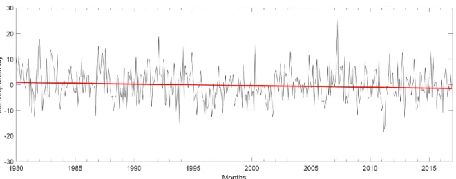
Figure 4.2 – SST anomaly averaged over the ABA region for the time period between September 1981 and December 2016. Red line represents the Theil-Sen regression. ... 19
Figure 4.3 – As in Fig. 4.2, but for the jet wind anomaly, regarding the climatology 1980-2016. ... 19
Figure 4.4 – As in Fig. 4.3, but for the jet frequency of occurrence anomaly. ... 20
Figure 4.5 – As in Fig. 4.3, but for the surface wind anomaly. ... 20
Figure 4.6 – Conditional probabilities of an intense surface wind given that: the jet does occur (a); the jet does not occur (b), and the probability that: the jet does not occur (c); the jet occurs (d), given that the surface wind is intense. ... 21
Figure 4.7 – 2-meter temperature (top panels) and respective anomaly (bottom panels) over the ABA region, averaged for the cases of strong (left), weak (centre) and neutral (right) jet. ... 21
Figure 4.8 – As in Figure 4.7 but for the sea surface temperature and with black arrows on the top panels representing the jet wind speed anomaly field for each case, respectively. ... 22
viii
Figure 4.9 – Surface pressure over the SE Atlantic Ocean (top), and its respective anomaly field over the Benguela (middle) and ABA regions for strong (left), weak (centre) and neutral (right) jet. ... 23 Figure 4.10 – As in Figure 4.7 but for the latent heat flux. ... 24 Figure 4.11 – Sensible heat flux anomaly field in the ABA region for cases of strong (left), weak (centre) and neutral (right) jet. ... 25 Figure 4.12 – As in Figure 4.11, but for the specific humidity anomaly. ... 25 Figure 4.13 – As in Figure 4.7, but for the momentum flux anomaly. ... 26 Figure 4.14 – Sea surface temperature (top panels) and respective anomaly field (bottom panels) averaged over the Benguela Niño (left), Niña (centre) and neutral (right) cases. ... 27 Figure 4.15 – As in Figure 4.14 (bottom panels), but for the 2-meter temperature anomaly field. ... 28 Figure 4.16 – As in Figure 4.14 but for the surface pressure in the Benguela region. ... 28 Figure 4.17 – Surface wind speed anomaly (top panels) and jet wind speed anomaly (bottom panels) averaged over the Benguela Niño (left), Niña (centre) and neutral (right) cases. The black arrows represent the wind speed anomaly field and the colours the magnitude of the anomaly. ... 29 Figure 4.18 – As in Figure 4.15, but for the specific humidity anomaly. ... 30 Figure 4.19 – As in Figure 4.15, but for the latent heat flux anomaly. ... 30 Figure 4.20 – As in Figure 4.15, but for the sensible heat flux anomaly over the sea (top panels) and for the whole ABA region (bottom panels). ... 31 Figure 4.21 – As in Figure 4.15 but for the momentum flux anomaly. ... 32 Figure 4.22 – Probability density functions for the anomalies of jet frequency of occurrence (top) and of jet wind intensity (bottom) for the composites of Benguela Niña (blue), Niño (orange) and neutral (yellow), and full time series (purple). ... 33 Figure 4.23 – Vertical distribution of the wind speed intensity (left panels) and its anomaly (right panels) for the west-east cross section at the jet northern core, averaged for the cases of strong (top), weak (middle) and neutral (bottom) jet. Grey area is the topography represented with the 1 arc-minute global model ETOPO1. ... 34 Figure 4.24 – As in Figure 4.23, but for the zonal wind component. ... 34 Figure 4.25 – As in Figure 4.23 (right panels), but for the potential temperature anomaly. ... 35 Figure 4.26 – As in Figure 4.23, but for the omega fields and overlaid with the jet wind speed (left panels) and anomaly (right panels) contour lines. ... 35 Figure 4.27 – Vertical distribution of the wind speed anomaly for the west-east cross section at the jet northern core, averaged over the Benguela Niño (top), Niña (middle) and neutral (bottom) cases. ... 36 Figure 4.28 – As in Figure 4.27, but for the potential temperature anomaly. ... 36 Figure 4.29 – As in Figure 4.26, but for the zonal wind (left panels) and its anomaly (right panels) of each SST composite. ... 37 Figure 4.30 – As in Figure 4.29 but for the omega field. ... 37 Figure 4.31 – Mean annual cycle of potential temperature from the surface up to 3 km, when jet occurs, averaged for the full period (first panel), Benguela Niño (second panel), Niña (third panel), and neutral (fourth panel). The black line indicates the jet height, respectively for each case. ... 38 Figure 4.32 – Distributions of jet height (left) and wind speed (right) for the full, Niño, Niña and neutral cases, respectively. The median values are indicated by the horizontal line inside each box, the first and third quartiles are indicated by the bottom and top sides of the box and the 10th and 90th percentiles by the whiskers. The small square inside each box indicates the mean value. ... 38
ix
Figure 4.33 – As in Figure 4.31, but for the wind speed. Black arrow indicates an example referenced in the text. ... 40 Figure 4.34 – As in Figure 4.31, but for the vertical gradient of potential temperature. Black arrow and red circle indicate an example referenced in the text. ... 41 Figure 4.35 – The first and third panels show the mean annual cycle of potential temperature from the surface up to 3 km, when jet occurs, averaged for Benguela Niño and Niña, respectively. The second and forth panels show the mean annual cycle of sensible (blue) and latent (orange) heat fluxes, averaged for the Benguela Niño and Niña, respectively. Black arrows indicate examples referenced in the text. ... 42 Figure 4.36 – As in Figure 4.35, but for wind speed on first and third panels. Black arrows indicate examples referenced in the text. ... 42 Figure 4.37 – As in Figure 4.35, but for the specific humidity (𝑞) and momentum flux (𝜏) on second and forth panels. ... 43 Figure 4.38 – As in Figure 4.37, but for the wind speed in first and third panels. ... 44 Figure 4.39 – As in Figure 4.37, but for vertical gradient of potential temperature in first and third panels.
... 44 Figure A1 – Cross-correlations between SST Niño 3.4 anomaly and: Benguela surface wind speed anomaly (left), and Benguela SST anomaly (right). ... 51 Figure A2 – Maximum correlation between SST Niño 3.4 anomaly and: Benguela surface wind speed anomaly (left), and Benguela SST anomaly (right). ... 51 Figure A3 – Vertical distribution of the wind speed intensity for the west–east cross section at the jet northern core, averaged for the cases of strong (top), weak (middle) and neutral (bottom) jet. ... 52
L
IST OF
T
ABLES
Table 3.1 – JRA-55 variables used in this work. ... 13 Table 4.1 – Values of jet height corresponding to the percentiles represented in Figure 4.32 (left). .... 39 Table 4.2 – Values of wind speed corresponding to the percentiles represented in Figure 4.32 (right). ... 39
x
L
IST OF
A
CRONYMS
ABA Angola-Benguela area
BCLLJ Benguela coastal low-level jet CLLJ Coastal low-level jet
EBC Eastern boundary current
EBUS Eastern boundary upwelling system
LLJ Low-level jet
MABL Marine atmospheric boundary layer
SAA South Atlantic Anticyclone
1
1. Introduction
The Benguela Coastal Low-level Jet (CLLJ) is a quasi-permanent atmospheric feature of the southeastern Atlantic, and has the second highest mean wind speeds of this jet type, after the Oman CLLJ (Lima et al., 2017). As its worldwide counterparts, it has a direct impact over its coastal climate, playing an important role in the interaction between land, ocean and atmosphere. From time to time, an El Niño-like phenomenon affects the Benguela upwelling system, particularly the Angola-Benguela region. The anomalous warming of the surface waters known as Benguela Niño disrupts the local ecosystems, and consequently brings socio-economic impacts. While each of the introduced phenomena have been studied separately, although not extensively, their relationship is still unknown. This work explores how the ocean surface and the marine atmospheric boundary layer respond to one another when affected by both the Benguela Niño and the Benguela CLLJ. The relationship between these two phenomena is also investigated. Given the biological and economic importance of this coastal upwelling region, it is paramount to understand the connection between the two highly-impactful features.
This thesis is organised as follows. In order to grasp the fundamental concepts explored in the current study, Section 2 provides an overview of the global upwelling systems (2.1), a brief description of the Benguela region and its main features (2.2), the forcing mechanisms of the Benguela Niño and its known impacts (2.3), an overview of coastal low-level jets, such as their location and driving mechanisms (2.4), and in a more detailed manner, the main properties of the Benguela CLLJ (2.5).
Section 3 is devoted to the data and methodologies used in the thesis to obtain the results, which are presented in Section 4 and discussed in Section 5 along with the final conclusions.
2
2. Fundamental concepts: an overview
2.1 Global Upwelling Systems
The ocean surface circulation along the eastern boundary regions of the subtropical oceanic gyres is the result of strong alongshore winds associated to the presence of semi-permanent high-pressure systems at those latitudes (e.g., the Azores High and the South Atlantic Anticyclone (SAA) at the North and South Atlantic, respectively). These mainly meridional and equatorward winds advect the upper ocean water offshore, by Ekman transport. As continuity of mass requires a replenishment of the advected water, deeper, denser and colder water surfaces. This process is known as upwelling, which is associated with an outcropping of the isopycnicals towards the coast, creating, in turn, an equatorward geostrophic surface flux: the wind-driven eastern boundary currents (Talley et al., 2011), as illustrated in Figure 2.1. Each of the four Eastern Boundary Upwelling Systems (EBUS) is, therefore, associated to its corresponding Eastern Boundary Current (EBC), as delimited in white in Figure 2.2. They include the California Current off the western North America coast and the Iberian/Canary Current along the western coasts of Iberian Peninsula and northern Africa, in the Northern Hemisphere. In the Southern Hemisphere, they encompass the Benguela Current off southwestern Africa and the Peru-Humboldt Current off western South America.
Figure 2.1 – Schematic of the coastal upwelling due to alongshore wind coupled with Ekman transport, in the Northern Hemisphere. Source: Talley et al., 2011.
The upwelling of subsurface water, colder and thus richer in nutrients than the original surface water, is a characteristic of the EBUS. Consequently, these regions are some of the most productive marine ecosystems in the Atlantic and Pacific oceans, contributing with more than 20% of the global capture fisheries, being essential habitats of marine biodiversity (Pauly and Christensen, 1995). Therefore, any change in the variability of the EBUS may have nefarious impacts on its highly vulnerable ecosystems and socio-economically, since there are about 80 million people living along the coasts near these systems (García-Reyes et al., 2015). In fact, in a recent study, Bakun et al. (2015) stated that the EBUS may suffer both physical and biochemical modifications due to the impacts of climate change, such as ocean stratification and variations on the surface wind field distribution.
3
Figure 2.2 – Mean surface pigment concentrations from the SeaWiFS ocean color sensor, averaged over its full mission (September 1997–December 2010), with the eastern boundary current systems (EBCs) outlined in white. Source: Strub et al.,
2013.
2.2 The Benguela region
The Benguela Current is a broad northward flow off southwestern Africa, part of the South Atlantic subtropical oceanic gyre, that develops near Cape Agulhas, at approximately 35ºS, and follows the coast towards the equator up to about 15º-16ºS, off the Angola coast (Fennel, 1999; Kämpf and Chapman, 2016). As in other eastern boundary currents, the Benguela Current is cold and driven by the eastern flank winds of the semi-permanent high-pressure system, the South Atlantic Anticyclone (SAA). However, it is most unique in the way that it is bounded by two warm currents, instead of one: the Agulhas Current to the south and the Angola Current to the north, separated from the latter by the sharp thermal Angola-Benguela Frontal Zone (Shannon et al., 1987; Reason and Smart, 2015). This permanent feature suffers a southward displacement during the late summer with the intrusion of the warm Angolan water into the Benguela current (Shannon et al., 1986), going as far as 17ºS, off the coast of Namibia (Shannon et al., 1987; Hardman-Mounford et al., 2003). As the other EBCs, the Benguela Current is accompanied by intense coastal upwelling and, therefore, high marine productivity (Kämpf and Chapman, 2016), crucial in supporting the livelihood of the people of Angola, Namibia and South Africa. In fact, it is estimated that the subsistence and commercial fisheries at the regional marine ecosystem had a direct economic impact of 517 million US dollars in 2006 (Sumaila, 2016).
The Benguela upwelling system comprises several cells along the southwestern African coast (Lutjeharms and Meeuwis, 1987). In the light of their study, and others, the Lüderitz cell, near 25ºS, is considered to be the most intense, with the lowest mean sea surface temperature (SST) of the eight wind-driven cells they identified in the southeast Atlantic, explained by the wide shelf and low eddy activity (Lachkar and Gruber, 2012). The northernmost is the Cunene cell, around 18ºS, where the Ekman drift is maximum, similarly to Lüderitz cell (Parrish et al., 1983).
The Namib Desert is a narrow coastal desert, about 50 to 150 km wide. To the east, it is limited by steep topography, with coastal mountains surpassing 1000 m of elevation (Figure 2.3). To the west, it is bounded by the northward-flowing Benguela current. During summer months, as with other subtropical deserts, there is an intense surface heating due to higher solar insolation, which leads to increased outgoing longwave radiation. The air above the surface warms and expands both vertically and horizontally, which in turn reduces the air density (Ackerman and Knox, 2003). The surface pressure decreases until there is a difference of 3 to 10 mb (sometimes even greater) in comparison with the surrounding areas. Due to its nature, this mechanism is often called thermal (or heat) low (Warner, 2004).
4
Figure 2.3 – Representation of the Benguela region bathymetry (blue hues) and topography (green to brown) with the 1 arc-minute global model ETOPO1. Red line represents the cross-section studied in this thesis.
The South Atlantic Anticyclone (SAA), particularly intense during the summer, is another atmospheric feature affecting the Benguela upwelling system, aside from the continental thermal low. This subtropical high-pressure system has a well-defined seasonality and strongly influences both the wind stress and SST fields off southwestern Africa, due to the prevailing along-shore winds that force the upwelling of the coastal waters (Risien et al., 2004).
2.3 Benguela Niño: an El Niño-like phenomenon
Every few years, an anomalous warming of the ocean surface occurs over the central and eastern equatorial Pacific, persisting for many months, with several impacts over the local ecosystem and climate (see Section 2.3.2). This phenomenon is known as El Niño and has been extensively studied (e.g., Trenberth, 1997; Yeh et al., 2009; Wang et al., 2012). In the equatorial Atlantic, there is also a similar phenomenon, termed the Atlantic Niño (e.g., García-Serrano et al., 2013), which will be discussed further but is not the main subject of this study. In the last decades, several authors have drawn attention to the occurrence of El Niño-like events in the southeast Atlantic, in the upwelling region of Angola-Benguela, which disrupts the climate (Nicholson, 1997; Reason and Smart, 2015) and the local ecosystems, with impacts on the marine productivity (Binet et al., 2001). In spite of being less frequent and less intense than the El Niño (Shannon et al., 1986) given the similarity to its Pacific counterpart and its location, this phenomenon has been termed Benguela Niño (Shannon et al., 1986). For the same reason, an anomalously cold water event is termed Benguela Niña, following the La Niña in the Pacific.
2.3.1 Forcing mechanisms
Although some Benguela Niño events have already been studied, there is still no consensus about their forcing mechanisms, of local or remote origins, or even if the Benguela Niño is a standalone phenomenon or a southward extension of the Atlantic Niño (e.g., Lübbecke et al., 2010), which occurs in the equatorial region of this oceanic basin.
5
Several hypotheses regarding the remote mechanisms which may force the Benguela Niño events have been suggested, mostly based on the inter and intra-basin relationships between the equatorial Pacific and Atlantic, the equatorial and southeast Atlantic (i.e., the Benguela region), and the equatorial Pacific and southeast Atlantic (Figure 2.4).
Through a time-space analysis of the evolution of the El Niño-Southern Oscillation (ENSO) signal in the Indic and Atlantic oceans, Nicholson (1997) suggested a connection between the Atlantic and the Pacific basins. The study shows that the equatorial Atlantic reaches its maximum cooling at the end of the year preceding the year of maximum warming on the Pacific (El Niño year). Furthermore, the maximum positive SST anomalies in the equatorial Atlantic are reached at the beginning of the year following the El Niño episode. Polo et al. (2014) added that an Atlantic Niño precedes a La Niña event in the Pacific, with a lag of six months between the two occurrences, assigning an order of events. On the other hand, Wang (2006) found no correlation between the Pacific and the Atlantic Niños, but states that the inter-basin SST gradient may influence tropical climate variability, instead of individual surface temperature anomalies.
A connection between the anomalous warmings of the Pacific and the Benguela coast is also a discussed topic. With NCEP reanalysis as input for the ocean model ORCA2, Colberg et al. (2004) showed that both the South Atlantic Ocean and its high-pressure system respond to an El Niño phase in the Pacific, with SSTs reaching their maximum at the end of the same year, and a weakening of the anticyclone throughout the year, thus changing the surface heat fluxes with a one-season lag. These results are mostly in agreement with Nicholson (1997). Nonetheless, the relationship between these events and the development of Benguela Niños is still not clear.
Using an ocean general circulation model together with satellite derived SST and sea surface height data, Florenchie et al. (2003) concluded that the anomalous warming which led to the Benguela Niños of 1984 and 1995 was originated near the equator, at a depth exceeding 50 m. This signal had progressed eastwards with a propagation rate consistent to the theoretical phase speed value of an equatorial Kelvin wave, until it reached the western coast of Africa, still in-depth. There, the warm anomaly started its propagation poleward, ascending to the surface at the Benguela region as a Benguela Niño event.
Lübbecke et al. (2010) agreed with the formation mechanism proposed by Florenchie et al. (2003), and added that the propagation of the Kelvin wave is caused by a modification of the trade winds intensity. These authors stated that the warm events at Benguela are preceded by a weakening of the South Atlantic Anticyclone (SAA), the dominant wind system over the basin, which comprises the midlatitude westerlies, the equatorward winds along the west coast of southern Africa and the south-easterly trade winds. A weakening of the anticyclone weakens the trade winds as well, generating
Figure 2.4 – Schematic of the inter and intra-basin relationships proposed to explain Benguela Niños mechanisms.
Equatorial Atlantic
Benguela Equatorial
6
equatorial Kelvin waves, which propagate eastward (Wang, 2002), deflecting the thermocline. The equatorial Atlantic SSTs will, therefore, increase, as well as the latent heat flux to the atmosphere (Florenchie et al., 2004).
Shannon et al. (1986) referred that changes in the alongshore local winds do not explain SST variations in the Angola-Benguela region. However, based on a coupled ocean-atmosphere model and satellite observations, Richter et al. (2010) argued that meridional anomalies in the local wind field are important for the development of a Benguela Niño event. These anomalies would weaken the South Atlantic high-pressure system, causing a warming at the Benguela coast 2 to 3 months later. Even though the authors do not discard the importance Kelvin waves might have on the development of warm events, they claim a variation on the local wind field has a great impact over the two regions.
2.3.2 Impacts
An abnormal increase in sea surface temperature along an upwelling region is a disturbance to the balance already established and brings important consequences to local ecosystems. As the nutrient-rich upwelled water is replaced by saline, warm waters (Shannon et al., 1986), many species migrate in search of favourable conditions (Binet et al., 2001; Rouault et al., 2003; van der Lingen et al., 2006). Gammelsrød et al. (1998) reported that intrusions of warm waters have been associated with mortalities of sardine, horse mackerel and kob off the coasts of Angola and northern Namibia, and rock lobsters suffer significant mortality when migrating (Cockcroft, 2001).
Many authors also reported that anomalous warm-water events in tropical southeast Atlantic were connected to increased rainfall in coastal Angola and also in northern Namibia (e.g., Rouault et al., 2003; Reason and Smart, 2005; van der Lingen et al., 2006).
2.4 An overview of Coastal Low-Level Jets
The marine atmospheric boundary layer (MABL) is the lowest part of the atmosphere under the direct influence of the ocean surface (Stull, 1988), where turbulent fluxes control its interactions with the atmosphere (Collaud Coen et al., 2014). A low-level jet (LLJ) is a MABL mesoscale feature characterised by maximum wind speeds between 10 m/s and 20 m/s (Stull, 1988), typically found within the first 1000 m, but mostly below 500 m above sea level. Its vertical extension is in the order of hundreds of meters, while its typical horizontal extension is much larger, sometimes exceeding thousands of kilometres (Ranjha et al., 2013).
The identification and location of a LLJ may be achieved using many criteria, from a simple analysis of the vertical profile of the horizontal wind, where one can determine where the maximum velocity occurs (Bonner, 1968; Stull, 1988), to more complex categorizations, based on the spatial location of the jet, its structure (both horizontal and vertical), period of occurrence, and its physical mechanism of formation (Ranjha et al., 2013; Semedo et al., 2016; Lima et al., 2017). Several hypotheses have been proposed on what forces the LLJs, from topographic forcings to inertial oscillations on the planetary boundary layer (Stull, 1988; Stensrud, 1996). Frequently, more than one mechanism can contribute to the jet formation, discerning a specific jet type which occurs over a certain region, during a specific period of time (Stull, 1988). The coastal low-level jets (CLLJ) are a type of LLJ and will be the one of the two main foci of this work.
Most of the studies on coastal low-level jets were locally developed, being the California CLLJ the one receiving the most attention. Consequently, the proposed methodologies only applied to those specific jet areas, and were not appropriate to perform a global analysis, as it would compromise the
7
accurate identification of all the CLLJs or their distinction from other types of low-level jet present in the same region. The first global climatology on the CLLJs was presented by Ranjha et al. (2013). They used the European Centre for Medium-Range Weather Forecasts (ECMWF) ERA-interim reanalysis as the input for an algorithm based not only on the horizontal wind profile but also on the vertical absolute temperature, since the presence of a CLLJ has a distinctive signature on both. As such, the proposed algorithm applied to atmospheric vertical profiles detects a CLLJ occurrence when the following criteria are met:
1. The jet maximum is found within the lowest 2 km of the troposphere; 2. The wind speed at the maximum is at least 20% higher than at the surface;
3. The wind speed above the jet maximum decreases to below 80% of that at the surface within 5 km above the maximum;
4. The temperature at the maximum is lower than at two model levels above (inversion detection);
5. The maximum temperature does not occur at the surface, as to verify the surface-based inversion.
The use of relative values of maximum speed for the jet definition, with a decrease starting at that level, allows an identification based on the behaviour of the wind speed profile, apart from the intensity values at that level, and helps prevent the so called false positives due to peaks in the wind speed at the level of the jet. Therefore, the presented set of criteria allows an objective identification of CLLJs, and can be applied to any vertical profiles. The global CLLJ frequency of occurrence distribution obtained from this methodology is shown in Figure 2.5.
Figure 2.5 – CLLJ frequency of occurrence (%) for (a) JJA and (b) DJF, with regions of interest enclosed in red. Source: Ranjha et al., 2013.
8
Coastal low-level jets typically occur along the eastern flank of subtropical semi-permanent high-pressure systems, at mid latitudes (e.g., Ranjha et al. 2013; Lima et al., 2017), along cold eastern boundary equatorward ocean currents. The presence of a thermal low over land, caused by intense heating of the surface mainly during summer months, and the high-pressure systems over the ocean are the main forcing mechanisms of along coast parallel winds, where the CLLJ occur (Lima et al., 2017). As such, these regions should be consistent with the location of each EBUS (Figure 2.2), and the respective wind-driven surface current. In fact, as show in Figure 2.5, CLLJs occur over well-known regions of coastal upwelling. In the Northern Hemisphere the areas of CLLJ occurrence can be found along the California current (California CLLJ; Winant et al., 1988; Parish, 2000) and the Canaries current (Iberian Peninsula and North Africa CLLJs, respectively; Soares et al., 2014). In the Southern Hemisphere, CLLJs can be found along the Humboldt current (Peru-Chile CLLJ; Garreaud and Munõz, 2005; Munõz and Garreaud, 2005), the Benguela current (Benguela CLLJ; Nicholson, 2010) and the western Australia (Western Australia CLLJ); Stensrud, 1996). The only CLLJ not located over an EBUS is the Oman CLLJ, at the Arabian Sea (Ranjha et al., 2013; Ranjha et al., 2015). Moreover, while the other CLLJs are equatorward, the Oman CLLJ propagates away from the equator. This difference lies in its being under the influence of the boreal summer Indian Monsoon system, which forces a parallel flux along the Arabian Peninsula south-eastern coast, and the Somali non-coastal low-level jet (Findlater, 1969; Ranjha et al., 2013).
Figure 2.6 – Conceptual model of lower atmosphere for the coast of California during the day. Source: Beardsley et al., 1987.
Throughout the summer months, parallel along-shore winds cause the upwelling of deeper, colder waters near the coast. This will enhance cross-shore temperature and pressure gradients, as the thermally-induced low pressure system is present over land, leading to a local increase of wind speed and further lowering the sea surface temperature (Winant et al., 1988; Semedo et al., 2016). The latter generates a decrease of evaporation (or latent heat flux) and, consequently, water vapour content of the atmosphere over the ocean surface in these regions, in a positive feedback cycle. The warm, dry air of the subtropical high-pressure system of the basin subsides, establishing sharp temperature and humidity inversions when in contact with the cold well-mixed layer, thus capping the marine atmospheric boundary layer (Beardsley et al., 1987; Burk and Thompson, 1996), as shown in Figure 2.6. Since the coastal upwelled waters have lower temperatures, the air at the base of the inversion will be coldest nearshore and warmer both inland and offshore, tilting it towards the coast. The inversion will thus be shallower nearshore, occasionally at lower heights than the coastal mountain range (blocking the cross-shore wind component), allowing the development of a thermal wind. The local wind flow will therefore
9
be enhanced, reaching its maximum right below the base of the inversion, decreasing its intensity both offshore, where the MABL is thicker, and towards the surface, due to friction (Beardsley et al., 1987; Winant et al., 1988; Burk and Thompson, 1996; Semedo et al., 2016). This developing mechanism explains why coastal low-level jets are parallel to the coast, limited to the MABL and are generally located over coastal upwelling/eastern boundary cold current regions, as well as why they occur mostly during the summer, when the ocean-land temperature horizontal gradient is stronger.
On the other hand, the strong parallel winds restrict the advection of moist marine air inland. As a consequence, and even though this particular type of jet develops over the ocean, it is common to find dry, barren deserts in the neighbouring land. Such is the case of the Atacama and Peruvian deserts of South America and the Namib Desert of southwestern Africa, to name a few (Warner, 2004). Under these conditions, the occurrence of a coastal low-level jet may enhance the aridity of the nearby deserts already conditioned by the lack of evaporation due to the cold bordering currents.
2.5 Benguela Coastal Low-level Jet
Even though coastal low-level jets have been studied throughout the last decades, the Benguela CLLJ was only introduced and studied by Nicholson (2010). Since then, little has been published about this particular coastal wind structure, which occurs along the southwestern African coast.
2.5.1 Jet Structure
Nicholson (2010) analysed the wind field in the Benguela region using data from the NCEP-NCAR reanalysis, which has a spatial resolution of 1º latitude x 1º longitude, together with SST data from the NOAA Extended Reconstructed Sea Surface Temperature dataset. The author revealed some characteristics of the Benguela jet, referring that its core is best developed in October, at 1000 hPa, where mean wind speeds exceed 10 m/s. The jet winds are mainly southeasterly, parallel to the coast of Namibia, thus covering the strong upwelling region, and extend over a large area of the South Atlantic (Figure 2.7).
Figure 2.7 – (a) Mean vector winds (m/s) and (b) SST (ºC) for October in southeastern Atlantic. Contours indicate speed. Values averaged for the period 1948 to 2005. Source: Nicholson, 2010.
10
In a detailed analysis of the Benguela CLLJ based on observations, reanalyses and atmospheric model simulations, Patricola and Chang (2016) showed that the representation of the Benguela jet is highly dependent on the product chosen. Whereas products with horizontal resolution finer than ~2º identify two near-shore wind speed maxima, the ones with coarser resolution, such as the NCEP used by Nicholson (2010), do not represent this characteristic which is unique to the Benguela jet. To identify the reason behind the existence of two cores, the authors compared two Weather Research and Forecasting (WRF) simulations at 27 km: one in which the “real” coastline was represented, and the other with an exclusively meridionally oriented coastline at 17.5ºS. They found that in the latter case the northern jet maximum (at 17.5ºS) is not present.
Chao (1985) showed that when winds interact with either the coastal topography or changes in its orientation, such as the presence of a convex coastline (e.g., capes), their intensity and direction may alter. If the coast turns away from the alongshore low-level flow, the latter will respond by changing its direction and expanding horizontally. In doing so, the thickness of the MABL will decrease, accelerating the flow to supercritical speeds, in what is called in hydraulic theory the expansion fan (Figure 2.8). If, however, the coast curves outwards, the flow will be compressed and weakens as the MABL height increases, becoming subcritical. This mechanism is known as hydraulic jump (Winant et al., 1988; Rogerson, 1999).
Figure 2.8 – 3D perspective of the marine layer for a case study with expansion and compression of the MABL. Source: Winant et al., 1988.
When Patricola and Chang (2016) modified the originally convex coastline, the wind speed reduced at 17.5ºS, which is consistent with the absence of the hydraulic expansion fan, and enhanced both up and downstream of the modified coastline, indicating the absence of the hydraulic jump. Since the topography remains steep in both simulations and in the light of the theory described above, the authors conclude that the modification in the Benguela CLLJ structure arises from the non-convex geometry.
A recent study showed that the Benguela CLLJ is the second most intense coastal jet (after the Oman CLLJ), with 17 m/s mean wind speed (Lima et al., 2017). During the austral winter it is a relatively shallow jet, occurring frequently between 400 and 500 m above sea level. In the summer months, it is placed between 400 and 900 m. Overall, it extends about 300 km offshore, as indicated by the Rossby radius (Ranjha et al., 2013). Regarding its vertical structure, Patricola and Chang (2016) considered a vertical cross section at the grid point nearest to the northern jet core (17.5ºS), as it is quasi-permanent throughout the year. The higher resolution reanalyses place the wind speed maximum (indicative of the jet core) at 975 hPa, near the coast, instead of the offshore 1000 hPa core identified by the NCEP reanalyses (Nicholson, 2010).
11
2.5.2 Variability
The Benguela CLLJ (BCLLJ) presents a pronounced seasonal variability in both wind speed and location. According to the output meridional wind at 10 m from the SCOW climatology (1999-2009) used by Patricola and Chang (2016), the northern jet core is located at 17.5ºS near the coast and coincides with Cunene upwelling cell and the Angola-Benguela front. It persists throughout most of the year, but is more intense during the austral transition seasons. The southern maximum is located some degrees offshore at 25º-30ºS and coincides with the Lüderitz upwelling cell. It is stronger during the austral spring and summer. Both cores have maximum wind speeds greater than 8 m/s. In the summer and winter months, the jet is essentially southeasterly (Ranjha et al., 2013). The Benguela CLLJ is weaker in austral winter and the southern core is not present.
12
3. Data and methods
3.1 Data
3.1.1 NOAA OI SST V2 High Resolution Dataset
There are several sea surface temperature datasets available and updated to the present day, such as the Centennial In Situ Observation-Based Estimates of the Variability of SST and Marine Meteorological Variables v2 (COBE-SST2, Hirahara et al., 2014) and the NOAA Extended Reconstructed SST V4 (ERSST v4, Huang et al., 2015). The NOAA Optimum Interpolation Sea Surface Temperature V2 High Resolution Dataset (NOAA OI SST V2, Reynolds et al., 2007) was selected since it provides a finer spatial resolution of 0.25º x 0.25º and one of the objects of this study is a SST anomaly-based phenomenon in a relatively confined region. This dataset is anomaly-based on ocean temperature satellite observations from the infrared Advanced Very High Resolution Radiometer (AVHRR) and in situ platforms and it spans the period from September 1981 to the present.
To monitor the El Niño, the NOAA Climate Prediction Center uses the ERSST v4 dataset to compute the Oceanic Niño Index, an SST based index averaged over an area over the east-central Pacific (the Niño 3.4). For comparison reasons, the NOAA OI SST V2 and the ERSST v4 were averaged over the Niño 3.4 region and the result of the SST anomalies is depicted in Figure 3.1.
Figure 3.1 – SST anomaly for the Niño-3.4 region during the period September 1981 to December 2010. Datasets: NOAA High Resolution Dataset (orange) and Extended Reconstructed Sea Surface Temperature version 4 (blue).
The selected dataset (NOAA OI SST v2) has an overall good description of the main characteristics in the ERSSTv4. The few discrepancies between the two datasets may be attributed to the coarser 2º x 2º grid resolution of the ERSSTv4.
3.1.2 JRA-55 Reanalysis
Reanalyses have been widely used for researching the mechanisms of the earth’s climate system, the study of predictability, and climate monitoring (Kobayashi et al. 2015). Some known global reanalyses available include the National Centers for Environmental Prediction (NCEP) Climate Forecast System Reanalysis (CFSR; Saha et al. 2010), the ERA-Interim (Dee et al., 2011) produced by the ECMWF, and
13
the Japanese 55-year Reanalysis (JRA-55, Kobayashi et al., 2015) carried by the Japanese Meteorological Agency (JMA). Out of the three, the JRA-55 covers the longest period (1958 to the present) and has a high resolution (TL319, ~55 km). It also represents the surface winds in an improved manner, being the most similar to the high-resolution satellite-based Scatterometer Climatology of Ocean Winds (SCOW, Risien and Chelton, 2008), as shown by Patricola and Chang (2016). Therefore, this study uses the JRA-55 to analyse the MABL structure in general, and when influenced by the Benguela Niño and the BCLLJ. The JRA-55 was produced with the higher resolution version of the JMA Global Spectral Model in reduced gaussian grid with 60 vertical levels up to 0.1 hPa, and provides atmospheric analysis based on incremental 4D-Var assimilation scheme (Courtier et al. 1994) every 6 hours (Kobayashi et al. 2015). The surface and model level variables used are presented in Table 3.1.
Table 3.1 – JRA-55 variables used in this work.
Variable Surface Model
level 2-meter specific humidity X
2-meter temperature X
10-meter u-component of wind X
10-meter v-component of wind X
Geopotential height X
Latent heat flux X
Momentum flux X
Potential temperature X
Pressure X X
Sensible heat flux X
u-component of wind X
v-component of wind X
Vertical velocity X
3.2 Methodology
This thesis is focused on the properties of the MABL and how they are conditioned by the Benguela Niño and the BCCLJ. As such, a methodology capable of conveying the changes in the MABL during Niño and Niña events, and under the influence of different jet intensities is presented in this subsection.
3.2.1 Jet detection algorithm
When studying the global CLLJ climatology, Ranjha et al. (2013) proposed a jet detection method, already presented in Section 2.4, based on the analysis of the wind speed and temperature vertical profiles derived from the ERA-Interim Reanalysis. Although several studies (e.g., Soares et al., 2014; Ranjha et al., 2015) have successfully detected the occurrences of coastal low-level jets using this method, it reveals some limitations. As Patricola and Chang (2016) showed, the reanalysis used by Ranjha et al. (2013) under-forecasts the wind speeds, and the CLLJs strength may have been underestimated. Furthermore, false detections could have been obtained in regions where CLLJs should
14
not be present, such as continental areas. In a recent study, Lima et al. (2017) revised the algorithm presented by Ranjha et al. (2013), which forced the temperature at the jet maximum to be lower than that at two model levels above (inversion detection). These authors argued that forcing the temperature at the jet maximum to be lower than that at two model levels above (inversion detection) discard a jet if it occurs at the top of MABL or at the level below the top, where in fact a jet may occur (e.g., Burk and Thompson, 1996; Garreaud and Muñoz, 2005; Parish, 2000). Lima et al. (2017) redefined that criterion of the Ranjha et al. (2013) algorithm to “The jet maximum is within or at the top of the MABL temperature inversion”, which brought a slight increase in the detection of each coastal jet in all areas.
Lima et al. (2017) also used the JRA-55 reanalysis, among others, as input to the revised algorithm, of which results: the frequency of occurrence, its intensity and height, as well as the model level data when the jet occurred. In the current thesis, the Benguela CLLJ results produced by Lima et al. (2017) is used as base for the analysis of the jet properties and its relation with the Benguela Niño.
3.2.2 Regions of interest
In order to study if and how the Benguela Niño impacts the structure and variability of the BCLLJ, and vice-versa, an area comprising both the influence of the jet and SSTs was required. The Angola-Benguela Area (ABA; Figure 3.2 – orange box), widely used in different studies (e.g., Florenchie et al., 2003; Richter et al., 2010) fits this purpose best, as it harbours both the Benguela Niño events and the northern core of the CLLJ throughout the year. Other extended areas, both southward and eastwardly, were tested (not shown) but the signal of the phenomena was not as clear.
A larger area which resulted from the jet detection algorithm, described in the previous section, was also considered in this study, henceforth called Benguela Area (Figure 3.2 – blue box).
Figure 3.2 – Map with the region of occurrence of the Benguela Coastal Low-Level Jet (blue) and the Angola-Benguela Area (orange).
15
3.2.3 Building the Niños catalogue and SST composites
As the Benguela Niño is a phenomenon characterised by SST anomalies in the ABA region, these were calculated in each grid point of that area, relative to the monthly mean series between September 1981 and December 2016. After determining the mean spatial SST anomaly (Figure 3.3), the Niños catalogue was developed in similarity to the Oceanic Niño Index (ONI, NOAA Climate Prediction Center) methodology. Since the SST anomalies for the Niño-3.4 (over which the ONI is computed) and ABA regions have very similar statistical behaviours (Figure 3.4), it was decided to use the same approach. Therefore, a Benguela Niño (Niña) episode was defined as the period of at least 5 consecutive months with SST anomalies greater than + 0.5ºC (lesser than – 0.5ºC), on a 3-month running mean of the anomalies, previously calculated in the ABA region. The remaining months, i.e., the months not part of a Niño or Niña event, were considered as “neutral”. In total, there were identified 6 Benguela Niño, 9 Niña, and 16 neutral events.
Figure 3.3 – SST mean anomalies for time period of 09/1981 to 12/2016 for the ABA region. Positive values shown as red and negative as blue. Dashed lines indicate ± 0.5 ºC limits.
Figure 3.4 – Boxplots of the SST anomalies averaged over the Niño-3.4 (left) and the ABA (right) regions.
In order to assess how the MABL responds to the Benguela Niño and Niña, SST composites were computed based on the obtained catalogue. For the SST anomalies in the ABA grid, the months
16
(3.1) corresponding to Niño events were aggregated and averaged. The same was performed with Niña and neutral months, forming three composites in total.
3.2.4 Building the CLLJ catalogue and jet wind composites
To define the jet catalogue, some calculations were performed beforehand. Firstly, because the JRA-55 variables hold a value for each synoptic hour, and the outputs from the jet detection algorithm maintain this temporal resolution, the daily mean for the jet wind speed was computed. Secondly, the anomalies of the obtained series were calculated for each grid point in the ABA region for the period between 1980 and 2016. Finally, these values were spatially averaged when needed. The ABA jet is then classified as “strong” (“weak”) when the daily jet anomaly exceeds (is below) the 90th (10th) percentile.
The jet wind composites were obtained similarly to the SST composites. All days falling in the “strong” or “weak” category were grouped and averaged. The remaining days were considered “neutral”.
3.2.5 MABL properties: temporal and spatial analysis
In an initial survey of the jet wind properties (its intensity and frequency of occurrence) and their relationship with the SST, the previously assembled time series of the respective anomalies (averaged over the ABA region) were evaluated. The tendency of each time series was determined by the Theil-Sen linear regression estimator, following the procedure proposed by Gilbert (1987). This methodology estimates the true slope (i.e., the change per unit time) of a linear trend while ignoring the gross errors and outliers present in the data. To compute the Theil-Sen estimator, it is necessary to determine the slope estimates, 𝑄, for each station, defined in Equation 3.1 as:
𝑄 =𝑥𝑖′− 𝑥𝑖 𝑖′− 𝑖
where 𝑥𝑖′ and 𝑥𝑖are data values at times 𝑖′ and 𝑖, respectively, and where 𝑖′> 𝑖. The Theil-Sen estimator
is then defined as the median of 𝑄. These tendencies, however, should be analysed with caution, as the reanalyses have been proven to be somewhat biased under long-term trend monitoring (Bengtsson et al., 2004).
To better understand the local connection between the surface wind and the jet wind, four conditional probabilities were computed. The first two are the probabilities of an intense surface wind (𝐴), which is defined as greater than its 75th percentile for each grid point, conditioned on the following events: 1) the jet does occur (𝐵1) and 2) the jet does not occur (𝐵2). The remaining two are 3) the probability that
the jet does occur given that the surface wind is intense 𝑃(𝐵1|𝐴), and 4) the probability that the jet does
not occur given that the surface wind is intense, 𝑃(𝐵2|𝐴).
These quantities can be computed for each point in the region by the following ratios:
{
𝑃(𝐴|𝐵𝑖) =
𝑃(𝐴 ∩ 𝐵𝑖)
𝑃(𝐵𝑖)
, for cases 1) and 2) 𝑃(𝐵𝑖|𝐴) =
𝑃(𝐵𝑖∩ 𝐴)
𝑃(𝐴) , for cases 3) and 4)
where 𝑖 = 1, 2 depending on the case and assuming 𝑃(𝐵1) ≠ 0 and 𝑃(𝐵2) ≠ 0 on cases 1) and 2) and
assuming 𝑃(𝐴) ≠ 0 on cases 3) and 4), since the probability is not defined if the denominator vanishes. (3.2)
17
In order to investigate the Benguela Niño (and Nina) signal on the jet properties, the probability density function was calculated for the frequency of occurrence and jet wind speed anomalies for each SST composite, averaged over the ABA box. Since the input data consist of anomalies and not their original values, the Gaussian (or normal) distribution is the best fit, instead of the Weibull distribution, typically used when analysing wind speed data (Harris and Cook, 2014). The probability density function (PDF) of a normal distribution is given by:
𝒩(𝑥|𝜇, 𝜎2) = 1
𝜎√2𝜋𝑒
−(𝑥−𝜇)2
2𝜎2
where 𝜎2 and 𝜇 are, respectively, the variance and the mean of the input series 𝑥 (Evans et al., 1993).
Because the MABL is under the direct influence of the ocean surface, any anomalous changes of the latter, for example, the occurrence of an Benguela Niño event, may perturb the physical properties of the MABL, such as the Benguela CLLJ, and vice-versa.
To understand how the surface and its fluxes are affected by the CLLJ, the properties of interest were applied to the jet wind composites. For this purpose, the SST, 2-meter temperature and specific humidity, surface pressure, surface momentum flux, and latent and sensible heat fluxes time series were averaged over each group of composites. For the JRA-55 variables, their respective anomalies were calculated regarding the period 1980 to 2016. Both the original SST values and their anomalies were conditioned to the jet wind composite. The same methodology was followed for the SST composites, this time to study the surface properties response to the Benguela Niño and Niña.
As the jet is a low-level feature, a surface analysis is insufficient to fully comprehend how it may be connected to the El Niño-like events in Benguela. Moreover, for a further understanding of the interaction between the surface and the low troposphere under the influence of such features, a vertical view is required. To this end, considering that the MABL structure is described by the model levels variables, each of these properties (Table 3.1) was computed for the jet wind composites. Since the northern jet wind maximum is the one that overlaps the area of occurrence of the Benguela Niño, the grid point closest to this core (17.5ºS) was chosen to study the ABA west-east cross-sections (Figure 2.3) for the composite-averaged variables. In addition, for this specific analysis and the next, the SST composites were redefined. Instead of the presented in Section 3.2.3, the composites were computed regarding the months of Niño, Niña and neutral, coincident with the jet occurrence. They were then gathered and temporally averaged, as the original methodology.
Finally, following the same input as the aforementioned analysis, the annual climatology of the SST and jet wind composites were computed for the full MABL. With this approach it is possible to observe the evolution of the different MABL properties throughout the year in the three SST composites, when the Benguela CLLJ occurs. As a proxy to the MABL inversion height, the vertical gradient of the potential temperature was obtained, and the jet height was studied in its context. To complete, the surface variables momentum, sensible and latent heat fluxes and specific humidity were also calculated for the annual climatology of each SST composite. This final analysis allows a simple yet insightful onlook of the ocean-atmosphere interaction when both the Benguela Niño and the BCLLJ occur.
18
4. Results
The original purpose of this work was to establish a relationship between the Benguela CLLJ and Benguela Niño, as well as between the Humboldt CLLJ and the El Niño, and possibly the connection between El Niño events and the Benguela CLLJ, as suggested by Nicholson (2010). There was effectively work done regarding El Niño and the BCLLJ, and Humboldt, but the results were weak and overall not satisfactory. Cross-correlations between the area-averaged Niño-3.4 SST and the Benguela surface wind series (and their respective anomalies) were calculated, in order to understand if there was some evidence of the referred influence of the El Niño over the wind (surface and low-level) in Benguela, albeit through simple methods. The maximum correlation values resulting from the cross-correlation analysis were always inferior to absolute 0.5 (Figure A1), and the cross-correlation obtained for the whole series was inferior to absolute 0.1 for all the combinations made with the variables. The maximum correlation value corresponded to a monthly-based lag between the two input series. For this specific lag, the Niño-3.4 averaged SST was correlated to each grid point of the Benguela region, for the SST and surface wind speed (Figure A2). Again, the results were weak and this study was not pursued further. Because the dynamics involved in the Humboldt and Benguela regions are different, it was decided that the study should be focused in only one area. This way, the ocean-atmosphere dynamics during a Niño and CLLJ occurrences would be conducted more thoroughly. Due to its much-discussed importance and lack of understanding on this particular region, this work settles on the Benguela area and the interaction between Benguela Niño events and the CLLJ.
Figure 4.1 – Seasonal Benguela Coastal Low-Level Jet properties: frequency of occurrence (a) and mean wind speed (b) for the Benguela region. For each group the 4 panels refer to the months of December to February (DJF), March to May
(MAM), June to August (JJA), and September to November (SON), as indicated on the top of each panel.
4.1 Benguela Coastal Low-Level Jet
The Benguela CLLJ, as aforementioned, is a quasi-permanent feature in the region. Figure 4.1 illustrates the seasonality of both the frequency of occurrence and the mean wind speed of the Benguela CLLJ. The presence of two wind speed maxima with distinct characteristics is clear. The maximum frequency of occurrence on the southern core takes place during the austral summer months, with frequency values exceeding 60%, whereas the northern core presents a maximum exceeding 50% but during the austral spring months. As for the wind speed, the southern core has stronger winds in general, with a mean exceeding 15 m/s on the austral summer and spring. However, it is less prominent on the
19
austral winter, although still stronger than the northern core, which has its peak on the austral spring, with a mean exceeding 13 m/s. Nevertheless, there is no doubt that the jet as a whole feature is present throughout most of the year, essentially due to its northern core, as shown by Patricola and Chang (2016).
4.2 Surface wind, low-level jet wind and the surface temperature
Investigating how the main properties of this work (SST and wind speed in ABA) have evolved over the years is crucial as a first step to understand the relationship of the Niño and the CLLJ in a global warming scenario. The Theil-Sen estimator for the SST anomaly shows an increase of 0.3ºC each decade, for the study period (Figure 4.2). Regarding the jet wind speed and frequency of occurrence anomalies, both time series have a negative tendency, of -0.4 m/s per decade (Figure 4.3) and -0.6% per decade (Figure 4.4), respectively. On the other hand, the surface wind speed anomaly time series (Figure 4.5) displays an increase (0.2 m/s per decade), showing an appearingly conflicting result.
Figure 4.2 – SST anomaly averaged over the ABA region for the time period between September 1981 and December 2016. Red line represents the Theil-Sen regression.