Spatial Variation of Longitudinal Dispersion in LECA-Based Vegetated Beds

Spatial Variation of Longitudinal Dispersion in LECA-Based Vegetated

Beds

António Albuquerque

1

Department of Civil Engineering and Architecture, University of Beira Interior, Edificio 2 das Engenharias, Calcada do Lameiro, 6201-001 Covilha, Portugal

[email protected]

Keywords: Dead volumes, dispersion, horizontal flow, MTS model, pollutant removal, vegetated

beds.

Abstract. The evaluation of the dispersion in vegetated beds may allow indentifying mechanisms that affect the transport and reaction of solutes, namely organic and nitrogen compounds. A set of non-reactive tracer experiments (slag injection) was performed in a vegetated bed (a mesocosm with a LECA-based substratum and colonized with Phragmites australis) used for the removal of organic and nitrogen pollutant loads. Loads of approximately 300 mg COD/L and 30 mg NH4-N/L and a hydraulic loading rate of 3.5 cm/d were used. The results showed a delay in all the residence time distribution (RTD) curves and a variation in the dimensionless residence time (µ(m,θ)) of the E(θ) curves, which means that the mass centre of the impulse was late relatively to the expected one. A strong dispersion and tracer retention (due to the presence of stagnated areas and internal recirculation) was observed, especially in the first 33 cm of the bed, which seems to have been related to the presence of complex clusters of roots, solid material, biofilm and LECA particles. An analytical solution of the Multiple-Tanks-in-Series (MTS) model well represents the RTD curves obtained in the tracer experiments. The detected dispersion and dead volume ratios (7% to 12%) did not affect the performance of the bed, which presented mean removal efficiencies of 85% and 60.4% for COD and NH4-N, respectively.

Introduction

Vegetated beds have been used for the control of stormwater runoff, stormwater discharge and wastewater treatment (domestic, industrial, landfill leachate and agricultural effluents), namely as vegetated channels, filters beds or constructed wetlands (CW) [1,2,3,4]. However, the substratum clogs frequently due to the type of material transported in the effluents, presence of biomass, retention of solid matter, precipitation of material and development of roots and rhizomes [1,5].

One of the most seriously problems of bed clogging occurs in the systems used for wastewater treatment, namely in horizontal subsurface flow (HSSF) vegetated beds [1,5], due to the development of stagnated volumes, dead volumes, hydraulic short-circuiting, internal recirculation and dispersion [1,2,6]. According to [7,8] light-expanded clay aggregates (LECA) have properties (high void ratio, porosity and specific surface area) that allow a better control of the clogging problem, as well as a better adhesion and growth of both biofilm and plants, which leads to the increase of the removal of organic matter, solids, nitrogen and phosphorous [7,8,9].

Tracer tests allow identifying the main mechanisms that are responsible for non-uniform distribution of flow and solutes in porous media wastewater treatment systems, which helps the better understanding of fluctuation in the performance of the beds or the yield loss, as observed in the studies of [1,6,10]. The identification of such mechanisms is based on the interpretation of the distribution of volume elements at the exit of some points of the system, using tools such as the Moments Method (MM) and consistency tests [6,11]. The longitudinal dispersion and the dead volume ratio may be estimated using non-ideal flow models as the Multiple-Tanks-in-Series (MTS) [1,6,11,12] through curve-fitting analytical solutions to E(θ) in θ curves obtained in tracer experiments.

All rights reserved. No part of contents of this paper may be reproduced or transmitted in any form or by any means without the written permission of TTP, www.ttp.net. (ID: 193.137.97.190-13/04/12,16:11:30)

The objective of the paper is to evaluate the longitudinal dispersion and the dead volume ratio in different sections of a LECA-based vegetated bed and to assess eventual interferences of these mechanisms on the removal of organic matter (as chemical oxygen demand (COD)) and nitrogen (as ammonia nitrogen (NH4-N)) along the bed.

Material and Methods

Tracer Experiments. A HSSF mesocosm with 1.9x0.8x0.5m (length, width, height), nine internal sampling points (IP1 to IP9) was used. The bed was filled with LECA (Filtralite NR 4-8 mm, specific surface area of 1 250 m2/m3), had 0.137 m3 of effective volume (void ratio of 0.45) and the water table was fixed in 0.2 m. The bed was first planted with Phragmites australis and the experiments started one year after the start-up (i.e. roots were well developed). Three internal points IP2 (0.33 m away from inlet), IP 5 (1 m away from inlet) and IP8 (1.90 m away from inlet) were used in these experiments. A scheme of the set-up may be seen in [6,9].

All the experiments were run with the bed fed with a synthetic wastewater based on sodium acetate and ammonia chloride and a flow-rate (Q) of 1 L/h (i.e., a hydraulic loading rate of 3.5 cm/d) and loads of 300 mg COD/L and 30 mg NH4-N/L. The tracing procedure included a slag injection of 500 mL of a sodium chloride (NaCl) concentrated solution (Co = 100 g/L) at the entrance, being the response evaluated by on-line measurement of conductivity at equal time periods of 1 minute, using a fixed conductivity TetraCon 325 probe and a Multi 340i meter (WTW, Germany). The experiments were conducted for three bed lengths (Inlet– IP2, Inlet– IP5 and Inlet– IP8), which corresponds to the theoretical hydraulic retention time (τ) of 1, 3 and 5.7 days.

At the beginning, middle and end of each tracer experiment, water samples were collected at the entrance and in the sampling points to evaluate pH, dissolved oxygen (DO), COD and NH4-N (i.e. 3 samples for each assay). pH and DO were measured directly through the probes SenTix 41 and CellOx 325, respectively, connected to the Multi 340i meter (WTW, Germany). COD and NH4-N were determined with the cuvette-tests LCK 614 (50-300 mg COD/L) and LCK 303 (2-47 mg NH4 -N/L) following the standards DIN 38409-4 (COD) and DIN 38406-E 5-1 (ammonia) and a CADAS 50 spectrophotometer UV-Vis (HACH-LANGE, Germany).

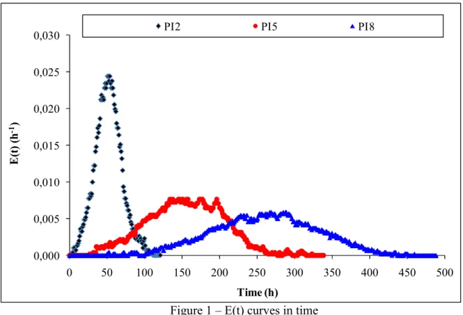
Residential Time Distribution Curves. The results from each experiment (conductivity in time) were converted into NaCl concentrations (mg/L) in time data using the respective calibration curve. These curves were afterwards normalized to obtain the corresponding residence time density functions (E(t)), also known as dimensional residence time distribution curves (RTD). The MM was used to estimate the first moment on the origin µm (mean residence time) and the second moment on the measuring point σ2 (variance) of the E(t) curve as presented in Fig. 1. In order to better compare the results of the different experiments, the reduced variance (σθ2) and the dimensionless curve E(θ) were computed. Table 1 presents the equations used for these calculations.

Table 1. Expressions to calculate the characteristics of the RTD curves for slag injections [1,11]

Name Parameter Expression

Dimensional RTD curve (h-1) E(t)

∫

∞ 0 dt ) t C( ) t C( ₍₁₎

Mean residence time (h) µm

∫

∞ • 0 t )d t E( t ₍₂₎ Variance in (h2) σ2

∫

Dimensionless RTD curve E_{(θ) µm•E(t) (5)}

0,000 0,005 0,010 0,015 0,020 0,025 0,030 0 50 100 150 200 250 300 350 400 450 500 E (t ) (h -1) Time (h)

PI2 PI5 PI8

Figure 1 – E(t) curves in time

Calculation of the Longitudinal Dispersion and Dead Volumes Ratio: The intensity of dispersion and the dead volume ratio may be known though the estimation of the number of tanks (N) in series of equal volume (V) and equally mixed and the active volume ratio (m), characteristics parameters of the MTS model, using curve-fitting techniques such as the nonlinear least-squares optimization method (LSOM).

The MTS model simulates the flow (Q) as it runs through the N tanks in series, admitting that solute concentration in the end compartment is given by Eq. 1 of Table 1. Admitting τi = Vi/Q and the conditions C(N+1) = 0, t = 0 and m as the ratio of active volume over total useful volume (i.e. the dead volume ratio (Vm) = 1-m), Eq. 7 gives an analytical solution for the MTS model that allow estimating N and m [10,11]:

(

)

Values of N below 4 indicate the presence of mixing conditions in the bed, whilst high values of N indicate that the regime is plug flow [1]. The N and m were estimated for each experiment using LSOM through curve-fitting Eq. 7 to E(θ) in θ curves. A simplification of the multi-purpose, nonlinear, least-squares method developed by Meeter, was used for curve-fitting Eq. 7 to experimental data. The optimization curve-fitting method considers a combination of the methods of Gauss-Newton and Levenberg-Marquardt as described in [6]. For a better comparison of the results the quadratic error (ξMD) was computed as presented in [13].

Results and Discussion

Residence time distribution curves. The results for each experiment are presented in Table 2. The values of µ(m,θ) provides information on the tracer retention inside the bed. All the values are above one, meaning that the mass centre of impulse was late relatively to the expected and is a typical response that indicates the presence of significant dispersion, as well as tracer retention in the bed substratum (due to adsorption or internal recirculation). Since the adsorption of NaCl was

considered negligible [6], the delay in the tracer exit may have been related to the presence of significant extensions of stagnated volumes (i.e. zones with low hydrodynamic activity that can develop into dead volume zones), as also reported by [1,9,10]. This circumstance may have caused internal recirculation, which retained part of the tracer inside those zones and also contributed to the longitudinal dispersion.

Table 2 – Characteristics of the RTD curves for all experiments

Section Duration of experiments (d) τ (h) µm (h) µ(m,θ) σθ 2 Inlet-IPI2 5.0 23.8 52.3 2.20 0.11 Inlet-IP5 14.1 72.0 155.0 2.15 0.11 Inlet-IP8 20.4 137.0 261.0 1.91 0.07

Therefore, the results suggest that the development of stagnated areas was more significant than the presence of dead volume areas. The dynamic of the bed has allow developing a complex matrix of Filtralite aggregates, biomass, roots and rhizomes, biofilm, filtered suspended solids and precipitates compounds that has contributed for the development of stagnated areas. These areas lead the appearance of mechanical dispersion phenomena where concentration gradients were developed during the flux of the tracer impulse, with the consequent transport of NaCl molecules into its interior and even into the grain’s porosity. When the disturbance left these areas, the tracer concentration was higher in the interior of the low irrigated areas than in its exterior, which provoked a gradient inversion, with the consequent diffusion of NaCl molecules into the exterior space. These tracer fractions consequently presented residence times higher than those of the fractions that accompanied the impulse front, which may help explaining the tracer retention in all the assays, as well the higher values of µ(m,θ) in all the bed sections.

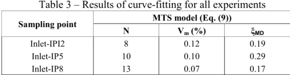
Longitudinal dispersion and dead volume ratio: The results for curve-fitting Eq. 7 to the experimental data are presented in Table 3.

Table 3 – Results of curve-fitting for all experiments

Sampling point MTS model (Eq. (9))

N Vm (%) ξMD

Inlet-IPI2 8 0.12 0.19

Inlet-IP5 10 0.10 0.29

Inlet-IP8 13 0.07 0.17

The adjustments were quite good, since the ξMD errors were low. According to [1,10,11] the longitudinal dispersion can be considered strong, since N was over 4 but close this value in all the sections. Dispersion and dead volume areas decreased throughout the bed’s length, being lower in the sections Inlet-IP5 and Inlet- IP8, where the presence of fewer roots was observed, which seems to indicate that the presence of roots and rhizomes may have had a beneficial effect on the control of hydrodynamic conditions over space, as also observed in [12]. It seems that there were mixing conditions in the bed’s initial section (first 33 cm of the bed), since the value of N was lower, which may be justified by a higher hydrodynamic disturbance due to the proximity of the feeding point.

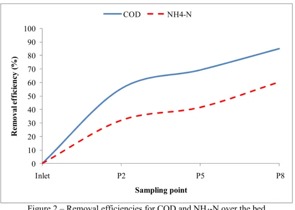
As shown in Fig. 2 the mean removal efficiency of COD (85%) was higher than the values observed by [8,9] and within the range of the values reported by [1,5] for HSSF beds (up to 95%). The average removal efficiencies of NH4-N (60.4%) were similar to the ones observed by [8], in the treatment of domestic wastewater, and by [9] in the treatment of synthetic wastewater, and higher than the ones reported by [1,5] for the treatment of domestic wastewater, which shows that ammonia oxidizers are very sensitive to operating conditions. This circumstance is related to the simultaneous occurrence of organic oxidation pathways (aerobic, anoxic and anaerobic), nitrification, denitrification, shortcut biological nitrogen removal, plant uptake, assimilation into biomass, filtration and sedimentation as discussed in [9].

0 10 20 30 40 50 60 70 80 90 100 Inlet P2 P5 P8 R em o v a l e ff ic ie n cy ( % ) Sampling point COD NH4-N

Figure 2 – Removal efficiencies for COD and NH4-N over the bed

The average mass removal rates of COD and NH4-N (calculated based on the influent and effluent concentrations, the flow rate and the effective area in each section) show that the removal of both compounds was higher in the initial section (Inlet-PI2) with 32.8 ± 0.5 g COD/m2.d and 2.1 ± 0.5 g NH4-N/m2.d where DO concentrations ranged between 1.2 and 2.5 mg O2/L, besides having been detected higher values of dead volumes (Vm) and dispersion in that section. Approximately 65% of the COD removal and 53% of the NH4-N removal occurred in the initial section.

Therefore, it seems that the presence of stagnated areas, internal recirculation, dead volume areas and strong dispersion, did not interfered with the performance of the Filtralite-based HSSF bed. One year after its start-up, the removal of COD and NH4-N was high.

Conclusions

The results show that there was a delay in the tracer exit in all the bed’s sections, which may have been related to the presence of stagnated areas and the occurrence of internal recirculation, due to the development of clusters of biomass, roots, rhizomes and solid material. The MTS model allowed concluding that the dispersion was very strong in the initial section of the bed, where mixing conditions may have occurred and higher values of dead volumes were registered. However, those conditions seem to have not interfered with the treatment performance of the Filtralite-based HSSF beds, which presented a high removal of COD and NH4-N, one year after the start-up.

Acknowledgments

This work was financed by the project PTDC/AMB/73081/2006 of the Portuguese Foundation for Science and Technology. We would like to thank the company Saint-Gobain Weber Portugal, S.A. for providing the Filtralite aggregates.

References

[1] R. Kadlec and S. Wallace: Treatment Wetlands (2nd edition, CRC Press, USA 2008).

[2] U.S. Environmental Protection Agency (USEPA): National Management Measures to Control

Nonpoint Source Pollution from Urban Areas (EPA-841-B-05-004, USA 2005).

[3] M.E. Barrett, A. Lantin and S. Austrheim-Smith: Transp. Res. Rec. Vol. 1890 (2004), p. 129. [4] A. Albuquerque, M. Arendacz, M. Gajewska, H. Obarska–Pempkowiak, P. Randerson and P.

Kowalik: Wat. Sci. Tech. Vol. 60 (2009), p 1677.

[5] J. Vymazal and L.Kropfelova: Wastewater Treatment in Constructed Wetlands with Horizontal

Subsurface Flow (Env. Pollution 14, Springer, Germany 2008).

[6] A. Albuquerque and R. Bandeiras, in: Water Pollution in Natural Porous Media at Different Scales, edited by L. Candela (Eds.), IGM, Serie 22, Madrid, Spain (2007), p. 329-338.

[7] R. van Deun and M. van Dyck: Proc. SWS Wetland Scientists, 29th June 2008, Saaremaa, Estonia, (2008), 23 pp.

[8] R. Vilpas, M. Valve and S. Raty: Pilot Plants in Finland (Technical report, Syke, MAXIT-Norden, Filand 2005).

[9] A. Albuquerque, J. Oliveira, S. Semitela and Amaral L.: Biores. Tech. Vol. 100 (2009), p. 6269.

[10] F. Chazarenc, G. Merlin and Y. Gonthier: Ecol. Eng. Vol. 21 (2003), p. 165.

[11] H. Fogler: Elements of Reaction Engineering (Bk&cdr, 3rd Edition, Prentice Hall Inc., New Jersey, USA 1999).

[12] P. Munoz, A. Drizob and W. Hession: Wat. Res. Vol. 40 (2006), p. 3209.