Application of Multivariate Statistical Methods in
Analyzing Business Surveys in Central Bank of
Nigeria
OGBUKA OBINNA RAYMOND
(M2015603)Dissertation report presented as partial requirement for
obtaining the Master’s degree in Statistics and Information
Management
Title: Application of Multivariate Statistical Methods in Analyzing Expectation Surveys in Central Bank of Nigeria Student OGBUKA OBINNA RAYMOND full name 201 6 201 6 Title: Application of Multivariate Statistical Methods in Analyzing Expectation Surveys in Central Bank of Nigeria Student OGBUKA OBINNA RAYMOND full name
NOVA Information Management School Instituto Superior de Estatística e Gestão de Informação Universidade Nova de Lisboa
APPLICATION OF MULTIVARIATE STATISTICAL METHODS IN
ANALYZING EXPECTATION SURVEYS IN CENTRAL BANK OF NIGERIA
by Ogbuka Obinna Raymond Dissertation proposal presented as partial requirement for obtaining the Master’s degree in Statistics and Information Management, with a specialization in Information Analysis and Management. Advisor / Co Advisor: Prof Jorge Mendes Co Advisor:DEDICATION
I dedicate this project to GOD, my late father Engr. G.O.L Ogbuka and my late brother Mr. Godwin Ogbuka who greatly inspired me to carry out this work. I also dedicate this project to my mother, Mrs L.A.R Ogbuka and all by siblings for their help and support financially and otherwise.ACKNOWLEDGEMENTS
I express my sincere appreciation to Dr. Sanni Doguwa, former Director Statistics Department, Central Bank of Nigeria (CBN), Dr. Olowofeso Olorunsola, Head Statistical Systems Management Division CBN, Prof. Joao Cadete Matos, Director Departamento de Estatistica, Banco de Portugal, all my colleagues in the Statistics Department, CBN and staff of Departmento de Estatistica, Banco de Portugal, for their help and support in making this project a reality.
Special thanks to my wife Ibe Chidinma Agnes, and my well wishers for their prayers and support
.
ABSTRACT
In analyzing survey data, most researchers and analysts make use of statistical methods with straight forward statistical approaches. More common, is the use of one‐way, two‐way or multi‐way tables, and graphical displays such as bar charts, line charts, etc. A brief overview of these approaches and a good discussion on aspects needing attention during the data analysis process can be found in Wilson & Stern (2001). In most cases however, analysis procedures that go beyond simple summaries are desirable. In this research work, data from 790 survey respondents who are purchasing managers in the manufacturing sector was analyzed using principal component analysis. The data spans Q32014 to Q22016.The result obtained enabled us to ascertain the factors that affect the manufacturing sector in Nigeria within quarterly period observations.
KEYWORDS
Principal components, Factor analysis, purchasing managers survey, eigen valuesINDEX
1. Introduction ... 6 2. Theoritical Framework ... 7 2.1. Literature Review ... 7 2.2. Objective ... 10 3. Study Relevance and Importance ... 11 4. Methodology ... 12 4.1. Description of Variables ... 12 4.2. Measurement Scale ... 12 4.3. Sample Size ... 13 4.4. Definision of Methods ... 13 4.5. Procedure and Steps ... 21 5. Results and discussion ... 26 5.1. Q3 2014 ... 26 5.2. Q4 2014 ... 29 5.3. Q1 2015 ... 31 5.4. Q2 2015 ... 34 5.5. Q3 2015 ... 36 5.6. Q4 2015 ... 38 5.7. Q1 2016 ... 41 5.8. Q2 2016 ... 44 5.9. Factor Summary ... 47 6. Conclusion ... 49 7. Limitations and Recommendations for future works ... 507.2. Recommendations for future works ... 50 8. Bibliography ... 51 9. Appendix ... 54 9.1. Q3 2014 ... 54 9.2. Q4 2014 ... 60 9.3. Q1 2015 ... 67 9.4. Q2 2015 ... 73 9.5. Q3 2015 ... 79 9.6. Q4 2015 ... 84 9.7. Q1 2016 ... 91 9.8. Q2 2016 ... 97
LIST OF TABLES
Table 5.1.1 ‐ Eigenvalues Matrix ... 26 Table 5.1.2 ‐ Factor Pattern Matrix ... 27 Table 5.1.3 ‐ Cronbach Alpha ... 28 Table 5.2.1 ‐ Eigenvalues Matrix ... 29 Table 5.2.2 ‐ Factor Pattern Matrix ... 30 Table 5.2.3 ‐ Cronbach Alpha ... 31 Table 5.3.1 ‐ Eigenvalues Matrix ... 32 Table 5.3.2 ‐ Factor Pattern Matrix ... 32 Table 5.3.3 ‐ Cronbach Alpha ... 33 Table 5.4.1 ‐ Eigenvalues Matrix ... 34 Table 5.4.2 ‐ Factor Pattern Matrix ... 35 Table 5.4.3 ‐ Cronbach Alpha ... 36 Table 5.5.1 ‐ Eigenvalues Matrix ... 37 Table 5.5.2 ‐ Factor Pattern Matrix ... 37 Table 5.5.3 ‐ Cronbach Alpha ... 38 Table 5.6.1 ‐ Eigenvalues Matrix ... 39 Table 5.6.2 ‐ Factor Pattern Matrix ... 40 Table 5.6.3 ‐ Cronbach Alpha ... 41 Table 5.7.1 ‐ Eigenvalues Matrix ... 42 Table 5.7.2 ‐ Factor Pattern Matrix ... 42 Table 5.7.3 ‐ Cronbach Alpha ... 43 Table 5.8.1 ‐ Eigenvalues Matrix ... 44 Table 5.8.2 ‐ Factor Pattern Matrix ... 45 Table 5.8.3 ‐ Cronbach Alpha ... 46 Table 5.9.1 ‐ Factor Summary ... 47LIST OF ABBREVIATIONS AND ACRONYMS
CBN Central Bank of Nigeria KMO Kaiser Meyer Olkin PCA Principal Component Analysis EFA Exploratroy Factor Analysis PMI Purchasing Manager Index IAS Inflation Attitudes Survey CES Consumer Expectation Survey BES Business Expectation Survey1.
INTRODUCTION
The major role of a Central Bank is to formulate monetary policies that positively impact the economic and social growth of a country. In formulating these monetary policies, useful data must be collected and analyzed. Data is usually collected through surveys and compulsory data renditions by participating entities. Most times the data is too large and complex and the analysis of this data is both time consuming and difficult, hence the need for the use of more robust scientific and statistical methods and procedures.
The Central Bank of Nigeria (CBN) aside from its price and monetary stability mandate is also tasked with supporting the Government’s policies on economic growth and unemployment reduction. This is done by using opinions and feedback from respondents to explore the general understanding of monetary policy issues. This is because good estimates and public understanding of what influences them are important parameters for successful monetary policy formulation.
This feedback is usually in the form of periodic surveys (monthly and quarterly) which are compared with other economic data in taking policy conditions. These surveys include Purchasing Managers Index survey (PMI) which is based on a survey of purchasing and supply executives of manufacturing and non‐manufacturing organizations, The Business Expectation Survey (BES) which provides advance indication of change in overall business activity in the economy, The Inflation Attitudes Survey (IES) which samples the views of households on their perception of the price change of goods and services within a period, and the Consumer Expectation Survey (CES) aimed at capturing an overall consumer confidence index.
This thesis will focus on the use of multivariate statistical analysis method namely ‐ factor analysis to extract useful information on the data realized from the conduct of the Purchasing Managers Index (PMI) survey in the manufacturing sector. The results of this analysis will facilitate knowledge of understanding the growth movement of the manufacturing sector in Nigeria and the factors that drive the growth in this sector and their impact on monetary policy formulation.
2.
THEORETICAL FRAMEWORK
2.1 LITERATURE REVIEW
The use of multivariate statistical techniques for analysis in various fields has greatly increased over the years. One of the mostly used techniques in multivariate statistical analysis is the Factor Analysis. Factor Analysis is a method for modeling observed variables, and their covariance structure, in terms of a smaller number of underlying unobservable (latent) “factors". The factors typically are viewed as broad concepts or ideas that may describe an observed phenomenon. Factor analysis is generally an exploratory and descriptive method that requires many subjective judgments by the researcher. Factor analysis is somewhat similar to principal component analysis in that the former is an inversion of the later. In factor analysis, we model the observed variables as linear function of the “factors”, while in principal components we create new variables (components) that are linear combinations of the observed variables.
Factor analysis is a widely utilized and broadly applied statistical technique in the social sciences and surveys. It is also prominently used in marketing, biological, agricultural, and financial applications, to name a few. In recently published studies, it has been used for a variety of applications, including developing an instrument for the evaluation of school principals (Lovett, Zeiss, & Heinemann, 2002), assessing the motivation of Puerto Rican high school students (Morris, 2001), and determining what types of services should be offered to college students (Majors & Sedlacek, 2001).
A number of research work has been done using Factor analysis. Bork and Moller (2012) examined the US housing price forecastability using a common factor approach based on a large panel of 122 economic time series. They found that a simple three factor model generates an explanatory power of about 50% in one‐quarter ahead in‐sample forecasting regressions. The predictive power of the model stayed high at longer horizons. The estimated factors were strongly statistically significant according to a bootstrap resampling method which took into account that the factors are estimated regressors.
Hassan et all (2012) focused on using the statistical technique ‐ factor analysis to construct the new factors affecting students’ learning styles of the survey done among university students. Their results showed seven new factors were successfully constructed using factor analysis and assigned as the factors affecting the learning styles; which are 1) students' attitude before and after attending class, 2) strategies used to comprehend the lecture, 3) the importance of lecture, 4) class size and its condition, 5) efforts outside class, 6) classroom convenient and 7) importance on listening to lecture.
Reuben and Pedro (2007) concluded that Parallel Analysis (PA) is one of the most recommendable rules for factor selection in Factor Analysis and Principal Component Analysis. However they said that this method is not available as an analysis option in the most commonly used statistical software packages. In view of that, they described a new, interactive and easy‐to‐use computer program capable of carrying out PA – the ViSta‐PARAN program.
Melanie Hof (2005) used two statistical methods namely Factor Analysis and Cronbach Alpha to evaluate a questionnaire used to determine Dutch seventh graders’ pleasure in writing. She concluded that although a questionnaire is generally accepted as reliable when the Cronbach alpha is higher than 0.8, we cannot claim that the questionnaire is valid based on the factor analysis alone. However, to prove that it measures one’s pleasure in writing, the results of other measures of one’s pleasure in writing should be compared.
Diana D. Suhr (2005) examined the basic differences between Principal Component Analysis (PCA) and Exploratory Factor Analysis (EFA). In her work, she inferred that Principal Component Analysis and Exploratory Factor Analysis are powerful statistical techniques. The techniques have similarities and differences. A priori decisions on the type of analysis to answer research questions allow you to maximize your knowledge.
Jill (2005) developed a new method for constructing measures of gender and women’s empowerment from cross‐sectional survey data using factor analysis. He re‐conceptualized gender and women’s empowerment for measurement purposes and argued that gender and women’s empowerment are best measured as a system of interrelated dimensions derived from context specific gender norms. The results of the confirmatory factor analysis were
used to construct weighted measures of women’s empowerment that are compared to simple scale measures
Rubén Daniel Ledesma (2007) described and illustrated how to determine the number of factors to retain in Principal Component Analysis (PCA) and Exploratory Factor Analysis (EFA). In his work, he applied the Monte Carlo simulation technique, Parallel Analysis, with an easy‐to‐use computer program called ViSta‐PARAN, a user‐friendly application that can compute and interpret Parallel Analysis.
Anna B. Costello and Jason W. Osborne (2005) looked at the best practices in Exploratory Factor Analysis. They aimed at collecting, in one article, information that will allow researchers and practitioners to understand the various choices available through popular software packages, and to make decisions about ‘best practices’ in exploratory factor analysis. They concluded that factor analysis, as well as other latent variable modeling techniques, can allow researchers to test hypotheses via inferential techniques, and can provide more informative analytic options.
Using the Regression model with many variables that are highly correlated with each other will not return the best estimators. The principal components that are to be taken into consideration are those factors that can explain the largest part of the information given by the initial variables. In this respect the number of factors which should be retained in the analysis is a decision matter for the researcher. For plotting purposes, two or three principal components deal with more variables that usually are correlated in order to reduce the dimension of the analysis to a small number of factors that are not correlated. Thus the negative effects of the multicollinearity are avoided. During factor extraction the total variance of a variable is split into two components; the shared variance between the variable and each factor and its unique variance (error variance). There are many extraction rules and approaches in the determination of the number of factors that are to be retained. One of the most popular is Kaiser’s criteria which state that only those factors with eigenvalue higher than the mean will be retained in the model. Also the Scree plot test, the cumulative percent of variance extracted will be used. Furthermore, a logical judgment would be involved in this selection process in order to determine the meaning of every factor retained in the model. For a better interpretation of the results, we would implore a rotational
method, which maximizes high item loadings and minimizes low item loadings. The rotation technique to be used is Orthogonal Varimax.
2.2 Objective
The clear objective of this work is to understand the pulse of the manufacturing sector and to empirically test and ascertain the factors that affect the growth of the manufacturing sector during the period Q32014‐Q22016, by obtaining and using the factors in the data that best describes this growth.
3.
STUDY RELEVANCE AND IMPORTANCE
The Central Bank of Nigeria (CBN) and indeed other central banks are tasked with administering monetary policies that will assist in maintaining price stability in an economy. One way this can be done is to check and regulate the amount of output in an economy. The central banks also establishes inflationary measures by tinkering the demand and supply of commodities. Through this study, knowledge of the degree of output from the manufacturing sector can give policy makers an idea of how to structure policies that affect general output.
Central banks also give monetary interventions to the real and manufacturing sector in order to boost output. This study can help to make these interventions more focused. For example, the relevant factors in this analysis of the survey explained the main factors responsible for the drive in the manufacturing sector. This can tell the area monetary interventions are needed.
This study is also important to the manufacturers in terms of knowledge of the level of employment and manpower in order to increase output.
4.
METHODOLOGY
For the purpose of this study, in applying the PCA and Factor analysis, the variables used are metric ones (likert scale). These variables represent factors that affect the manufacturing output in the manufacturing sector in Nigeria. The variables are represented as x1 to x11 as outlined below:
4.1 Description of Variables
1. Production Level – x1 2. Level of new orders or customers or incoming business received – x2 3. Suppliers’ delivery time – x3 4. Level of employment in organisation – x4 5. Raw materials inventory/work in progress – x5 6. New export order received – x6 7. Average price of outputs – x7 8. Average price of inputs – x8 9. Quantity of items purchased – x9 10. Level of outstanding business/Backlog of work in organization – x10 11. Stock of finished goods – x114.2 Measurment Scale
The variables will be measured using the likert scale with numbers form 1 – 3 assigned as outlined below: 1. Higher – 3 2. Same – 2:
:
:
:
:
:
:
:
Starting from the assumption that these variables are collinear, the purpose of the PCA is to reduce the number of variables that measure the factors affecting manufacturing output to a small number of factors that are not correlated.4.3 Sample Size
The sample size is derived from monthly questionnaire feedback from purchasing managers in 560 manufacturing businesses in Nigeria. We would use the mean of the monthly returns of 3 consecutive months to get a quarterly series, ranging from 2014Q3 to 2016Q2. Thus for each quarter, we have 560 data points.4.4 Definition of Methods
From our data let’s assume we develop a population variance‐covariance matrix similar to the one below;
1. VAR(X) = ∑ =
ơ1
2ơ12 ‘’’’’ ơ1p
Ơ21 ơ22 ‘’’’’ ơ2p
Ơp1 ơp2 ‘’’’’’’ ơp2 Considering the linear combinations,
Y
1= e
11X
1+ e
12X
2+ ... + e
1pX
pY
2= e
21X
1+ e
22X
2+ ... + e
2pX
pY
p= e
p1X
1+ e
p2X
2+ ... + e
ppX
p Each of these can be thought of as a linear regression predicting
Y
J fromX
1,X
2,...,X
p There is no intercept, but
e
j1, e
j2, ... ,e
j2 can be viewed as regression coefficients.p p p K=1 p l=j l=j P P Therefore it has a population variance. var(
Y
j) =
∑∑
ejk
ejl
ơ
kl= e’
j∑e
j Hence,
Y
jand
Y
kwill have a population covariance of
cov(
Y
j,Y
k) =
∑∑
ejkejl
ơ
kl= e’
j∑e
k In this case the coefficients
ejk
are collected into the vector
ej1
ejk = ej2
ej3
2.
FIRST PRINCIPAL COMPONENT (PC1) : Y1 The first principal component is the linear combination of x‐variables that has maximum variance (among all linear combinations), so it accounts for as much variation in the data as possible.
Specifically we will define coefficients
e11,
e12,
e13,
…..,e1p
for that component in such a way that its variance is maximized, subject to the constraint that the sum of the squared coefficients is equal to one. We require this constraint so that a unique answer is obtained.
Thus we formally select
e11, e12, e13,
…..,e1p
that maximizesvar(
Y
j) =
∑∑
e1k
e1l
ơ
kl=e’
1∑e
1j=1 K=1 K=1 k=1 l=j l=i l=i P P P P P P P j=1
e’1e1
=∑
e
21j =1
3.
SECOND PRINCIPAL COMPONENT (PC2) : Y2 The second principal component is the linear combination of x‐variables that accounts for as much of the remaining variation as possible, with the constraint that the correlation between the first and second component is 0.
We select
e21, e22, e13,
…..,e2p
that maximizes the variance of the new componentvar(
Y
2) =
∑∑
e2k
e2l
ơ
kl=e’
2∑e
2subject to the constraint that the sums of squared coefficients add up to one,
e’2e2
=∑
e
22j =1
along with the additional constraint that these two components will be uncorrelated with one another.
cov(
Y
1,Y
2) =
∑∑
e1ke2l
ơ
kl=e’
1∑e
2=0
4. j‐th
PRINCIPAL COMPONENT (PCj) : Yj Subsequently all principal components are now linear combination that account for as much of the remaining variation as possible and they are not correlated with the other principal components.
Hence generalizing, we have
ej1, ej2, ej3,
…..,ejp
that maximizesvar(
Y
j) =
∑∑
eikejl
ơ
kl=e’
j∑e
jl=j k=1 j=1 P P P P P P k=1 k=1 l=j l=j
:
:
:
:
:
:
:
:
with the additional constraint that this new component will be uncorrelated with all the previously defined components.e’1e1
=∑
e
21j =1
cov(
Y
1,Y
j) =
∑∑
e1kejl
ơ
kl=e’
1∑e
j=0
cov(Y
2,Y
2) =
∑∑
e2kejl
ơ
kl=e’
2∑e
j=0
cov(Y
j‐1,Y
2) =
∑∑
ej‐i,k ejl
ơ
kl=e’
j‐1∑e
j=0
Thus all principal components are uncorrelated with one another.
5.
FACTOR ANALYSIS AND PRINCIPAL COMPONENTS RELATIONSHIPEarlier on, Factor Analysis was defined as a method for modeling observed variables and their covariance structure, in terms of a smaller number of underlying unobservable (latent) “factors". It was also stated that Factor analysis is somewhat similar to principal component analysis in that the former is an inversion of the latter. In factor analysis, we model the observed variables as linear function of the “factors”, while in principal components we create new variables that are linear combinations of the observed variables.
The similarities between principal component analysis and factor analysis are outlined below:
Recall that our previous definition of principal components let to the equation below:
Y
1= e
11X
1+ e
12X
2+ ... + e
1pX
pY
2= e
21X
1+ e
22X
2+ ... + e
2pX
p:
:
:
:
:
:
Let
e’
k = (ek1
ek2 ek3 ... ekp
)be the p x 1 k‐eigenvector of the correlation matrix
R
, with the associated eigenvalueλ
k.
Therefore denoting
E
=(
e
1e
2 .... ep) then the definition of the principalcomponent is:
Y
=E’X
Where
X’ =
(X
1X
2.... X
p)
is the vector where we collected the observed variables,
Y’ =
(Y
1Y
2.... Y
p) is the principal components vector and
ʌ =
diag(
λ
1λ
2... λ
p)
isthe diagonal matrix containing the eigenvalues. As a consequence of the definition of the principal components,
E(Y) = 0 and Var(Y) =
ʌ
In order to have standardized principal components (leading to standardized scores), we have to provideY*
=
ʌ
‐1/2E’X,
Where
Y*’
=
(Y*
1Y*
2.... Y*
p) is the vector of standardized principal components.
Writing
X
as a function ofY*
, we have:
Y*
=
ʌ
‐1/2E’X
ʌ
1/2Y =
E’X
X =
E
ʌ
1/2Y
(we will denoteE
ʌ
1/2= L
) This means that the matrix of loadings of the factor model
L
is given bye
11√λ
1+ e
21√λ
2+ ... + e
p1√λ
pL =
e
12√λ
1+ e
22√λ
2+ ... + e
p2√λ
p:
:
:
:
:
P P P K=m+1 K=m+1 K=m+1 Ԑ2 Ԑ1 Ԑ3 The corresponding equations are:
X
1= e
11√λ
1Y
1*
+ e
21√λ
2Y
2*
+ ... + e
p1√λ
pY
P*
X
2= e
12√λ
1Y
1*
+ e
22√λ
2Y
2*
+ ... + e
p2√λ
pY
P*
X
P= e
1p√λ
1Y
1*
+ e
2p√λ
2Y
2*
+ ... + e
pp√λ
pY
P*
Alternatively,
X =
LY*’
,And each
e
jk√λ
k is the loading of the variable j on the principal component k,I
jk Using principal component to extract latent factors means we keep just the first m, leaving the remaining ones in a specific factor:
X
1=
e
11√λ
1Y1*
+ e
21√λ
2Y2*
+ ... + e
m1√λ
mYm*
+
∑
e
k1√λ
kYk*
X
2= e
12√λ
1Y1*
+ e
22√λ
2Y2*
+ ... + e
m2√λ
mYm*
+
∑
e
k2√λ
kYk*
X
P= e
1p√λ
1Y1*
+ e
2p√λ
2Y2*
+ ... + e
mp√λ
mYm*
+
∑
e
kp√λ
kYk*
We call factors to the initial retained standardized principal components,
Y*’ =
(Y1* Y2* .... Yp*) = f’ = (f1 f2 .... fp)
Furthermore, two main differences exist between principal component analysis and factor analysis. They include:
First, principal components analysis places emphasis on the explaining the variance in the data; the objective of factor analysis is to explain the correlation among the
:
:
:
:
Second, in principal components analysis the variables form an index. For example, in the following equation
Y
1= e
11X
1+ e
12X
2+ ... + e
1pX
pThe variables are called formative indicators of the component and the index is formed by the variables.
In factor analysis, on the other hand, the indicators reflect the presence of unobservable construct(s) or factor(s). For example, in the following equations:
X
1- µ
1=
l
11F
1+
l
12F
2+ ... +
l
1mF
m+ Ԑ
1X
2- µ
2=
l
21F
1+
l
22F
2+ ... +
l
2mF
m+ Ԑ
2X
P- µ
P=
l
P1F
1+
l
P2F
2+ ...+
l
PmF
m+ Ԑ
P Where the variables (X1, X2, ... Xp) are functions of the latent construct(s) or factor(s), (f1, ,f2,....fm) and the specific factors (Ԑ1, Ԑ2, ... Ԑp). In other words, they reflect the presence of the unobservable or latent constructs and hence the variables are called reflective indicators.6.
FACTOR ANALYSIS METHODOLOGYChua (2009) suggested that factor analysis is the procedure been used by researchers to organize, identify and minimize big items from the questionnaire to certain constructs under one dependent variable in a research. Kaiser Meyer Olkin KMO test was done to identify whether the data is suitable for factor analysis. The KMO test formula as stated by Norusis is:
KMO =
Where: ri2j = correlation coefficient∑
n J=1∑
ni=1r
i2j(∑
nJ=1∑
ni=1r
i2j+ ∑
nJ=1∑
ni=1a
i2j)
:
:
:
:
~
~
~
~
~
^ ^ : ^ ^ ^ ^ : : : ^ ^ ^ ^ ^ ^ ^ ^ ^~
~
~
(p X 1) (p X 1) (p X m) (m X m) ai2j = Partial correlation coefficient Recall that the factor analysis model as stated by Johnson and Wichern is:X
1- µ
1=
l
11F
1+
l
12F
2+ ... +
l
1mF
m+ Ԑ
1X
2- µ
2=
l
21F
1+
l
22F
2+ ... +
l
2mF
m+ Ԑ
2X
P- µ
P=
l
P1F
1+
l
P2F
2+ ...+
l
PmF
m+ Ԑ
P Johnson and Wichern stated the orthogonal factor model with m common factors as follows:X = µ + L F +
Ԑ
Where:µ
i = mean of variable iԐ
i= ith specific factorF
j= jth common factorL
ij = loading of the ith variable on the jth factor Johnson and Wichern (2002) also estimate the communalities as:h
i2=
l
2i1+ l
2i2+ ...+ l
2imThe principal component factor analysis of the sample covariance matrix S is specified in terms of its eigenvalue‐eigenvector pairs
(λ
1,e
1), (λ
2,e
2), ... ,(λ
3,e
3)
where(λ
1≥ λ
2≥ .. λ
p).
Let
m < p
be the number of common factors. Then the matrix of estimated factor loadingsl
is given by:
L = √(λ1e1) √(λ2e2) √ (λmem
)
Johnson and Wichern (2002) stated that the estimated specific variances are provided by the
S - LL',
~
Ѱ1
Ѱ
Ѱ2
Ѱp
~
~
~
:
^ J=1 m~
with
Ѱ
i= S
ii‐
∑ l
2ij4.5 Procedure/Steps
STEP 1: DESCRIPTIVE STATISTICS McClave et al. (2005) defined descriptive statistics as an approach that utilizes numerical and graphical methods to look for patterns in a data set, to summarize the information revealed in a data set, and to present the information in a convenient form. Altman et al. (2006) also stated that pilot study was a small experiment done to test the logic and to improve the information quality and efficiency collected from big study. STEP 2: RELIABILITY ANALYSIS Coakes and Ong (2011) suggested that reliability analysis was used to determine the internal consistency of the scales using Cronbach Alpha. The formula as stated by Fraenkel and Wallen (1996) is:rKk
=.
1
‐
where: rKk = estimated Cronbach Alpha coefficient value k = number of items in the questionnaire Si2 = sum of item variancesk
k ‐ 1
S
i2S
x20
0
0
0
0
0
. . .
. . .
. . .
:
:
=
^Sx2 = factor variances
STEP 3: INITIAL EXTRACTION OF THE COMPONENTS
In principal component analysis, the number of components extracted is equal to the number of variables being analyzed. Since eleven variables are analyzed in the present study, eleven components will be extracted. The first component can be expected to account for a fairly large amount of the total variance. Each succeeding component will account for progressively smaller amounts of variance. Although a large number of components may be extracted in this way, only the first few components will be important enough to be retained in order to determine the new factors.
STEP 4: DETERMINING THE NUMBER OF MEANINGFUL COMPONENTS TO RETAIN
Earlier it was stated that the number of components extracted is equal to the number of variables being analyzed, necessitating that there would be a decision of just how many of these components are truly meaningful and worthy of being retained for rotation and interpretation. In general, we expect that only the first few components will account for meaningful amounts of variance, and that the later components will tend to account for only trivial variance. The next step of the analysis, therefore, is to determine how many meaningful components should be retained for interpretation. The study will describe three main criteria that would be used in making this decision: the eigenvalue‐one criterion, the scree test, the proportion of variance accounted for.
A: The Eigenvalue‐One Criterion; In principal component analysis, one of the most
commonly used criteria for solving the number‐of‐components problem is the eigenvalue‐ one criterion, also known as the Kaiser criterion (Kaiser, 1960). With this approach, we would retain and interpret any component with an eigenvalue greater than the mean of eigenvalues.
The rationale for this criterion is straightforward. Each observed variable contributes one unit of variance to the total variance in the data set. Any component that displays an eigenvalue greater than the mean is accounting for a greater amount of variance than had
been contributed by one variable. Such a component is therefore accounting for a meaningful amount of variance, and is worthy of being retained.
On the other hand, a component with an eigenvalue less than the mean is accounting for less variance than had been contributed by one variable. The purpose of principal component analysis is to reduce a number of observed variables into a relatively smaller number of components; this cannot be effectively achieved if we retain components that account for less variance than had been contributed by individual variables. For this reason, components with eigenvalues less than 1.00 are viewed as trivial, will not be retained.
B: The Scree Test; With the scree test (Cattell, 1966), we would plot the eigenvalues
associated with each component and look for a “break” between the components with relatively large eigenvalues and those with small eigenvalues. The components that appear before the break will be assumed to be meaningful and would be retained for rotation; those appearing after the break are assumed to be unimportant and are not retained.
Sometimes a scree plot will display several large breaks. When this is the case, we would look for the last big break before the eigenvalues begin to level off. Only the components that appear before this last large break should be retained.
C: Proportion of variance accounted for; A third criterion to be implored in this study to
solve the number of factors problem involves retaining a component if it accounts for a specified proportion (or percentage) of variance in the data set. We will to retain any component that accounts for at least 50% to 60% of the total variance. This proportion can be calculated with a simple formula: Proportion = Eigenvalue for the component of interest Total eigenvalues of the correlation matrix In principal component analysis, the “total eigenvalues of the correlation matrix” is equal to the total number of variables being analyzed (because each variable contributes one unit of variance to the analysis. STEP 5: ROTATION
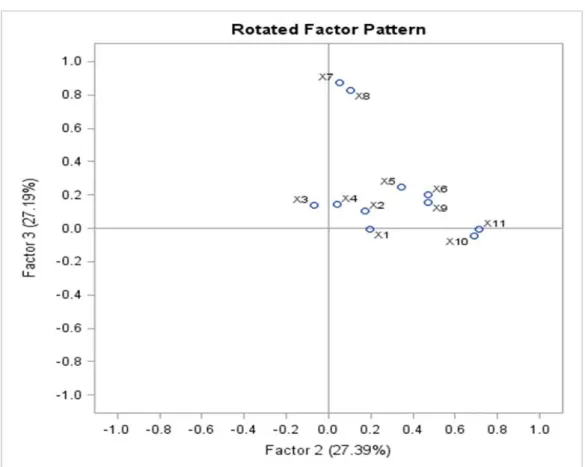
When more than one component has been retained in an analysis, the interpretation of an unrotated factor pattern is usually quite difficult. To make interpretation easier, we will perform an operation called a rotation. A rotation is a linear transformation that is performed on the factor solution for the purpose of making the solution easier to interpret. For software purposes, we would apply a varimax rotation which results in uncorrelated components. Compared to some other types of rotations, a varimax rotation tends to maximize the variance of a column of the factor pattern matrix (as opposed to arrow of the matrix).
STEP 6: INTERPRETING THE ROTATED SOLUTION
The rotated solution will be interpreted by determining what is measured by each of the retained components. Briefly, this would involve identifying the variables that demonstrate high loadings for a given component, and determining what these variables have in common. A name would be assigned to each retained component that describes its content.
The first decision to be made at this stage is to decide how large a factor loading must be to be considered “large.” Stevens (1986) discusses some of the issues relevant to this decision, and even provides guidelines for testing the statistical significance of factor loadings. For purpose of this study however, we would simply consider a loading to be “large” if its absolute value exceeds 0.5.
Finally we will carry out a reliablity anaysis of or internal consistency of the factors using Cronbach alpha. Based on the factor analysis, we want to use a subset of the items to assess the factors. This would enable us know how well the items from each factor hang together such that one can use a single composite score or further analysis. A useful rule states that a scale is reliable if it has a Cronchbach’s alpha of 0.70 or greater (Nunnally 1978). For the purpose of this project, we would use a Conchbach’s alpha of 0.70.
Furthermore, when performing reliability analysis, you might want to know which variables are the most and least useful in your scale. You can calculate alpha if item deleted by removing each variable in turn and computing alpha without that variable in the analysis. The higher the alpha if item deleted is, the less that target variable contributes to the
internal consistency of the scale. Conversely, a small alpha if item deleted suggests that the item is important to the reliability of the scale.
5.
RESULTS AND DISCUSSION
5.1 Q3 2014
We would consider the data from Q3 2014 to be suitable for Factor Analysis, because looking at the overall data quality measure – KMO (Table 9.1.2), the value obtained is approximetely 0.766 which is suitable.
The table displaying the correlations and relationship between each of the various variables in the data is also displayed in Table 9.1.3
Recall that from the eigenvalue‐one criterion otherwise known as the kaiser criterion, we would retain and interprete any component with an eigenvalue greater than the mean (in this case greater thatn one).
Tabel 5.1.1. Eigen values Matrix
Eigenvalue Difference Proportion Cumulative
1 3.27817784 1.81756 0.29800 0.298 2 1.46061766 0.30427811 0.13280 0.43080 3 1.15633955 0.17757367 0.10510 0.53590 4 0.97876588 0.17480878 0.08900 0.62490 5 0.8039571 0.09451569 0.07310 0.69800 6 0.7094414 0.05511039 0.06450 0.76250 7 0.65433102 0.04353682 0.05950 0.82200 8 0.61079419 0.00561358 0.05550 0.87750 9 0.60518061 0.14232947 0.05500 0.93250 10 0.46285114 0.18330752 0.04210 0.97460 11 0.27954362 0.02540 1
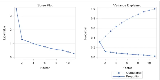
From the table 5.1.1 and using the Kaiser criterion, we can evidently see that the first, second and third factors have eigenvalues greater than 1 and hence would be retained. These factors account for 53.6% of the total variability of all the variables.
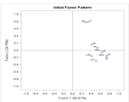
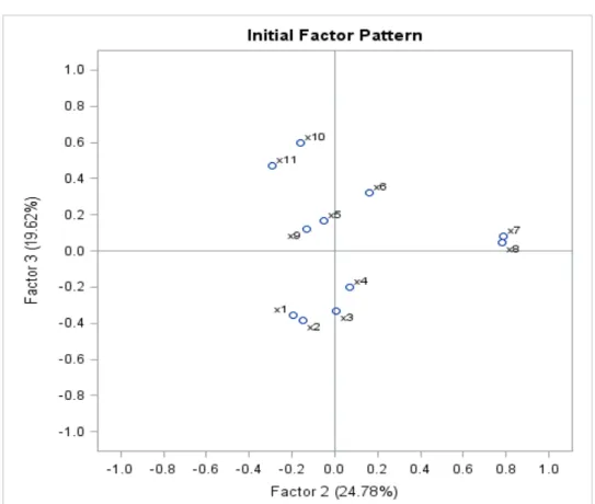
Furthermore, the scree plot of the eigenvalues and factors shows that the number of factors to be retained is the data points that are above the break (i.e point of inflexion). To determine the break, we can draw an imaginary horizontal and vertical line from each end of the grap
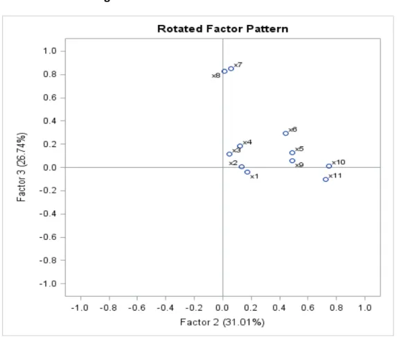
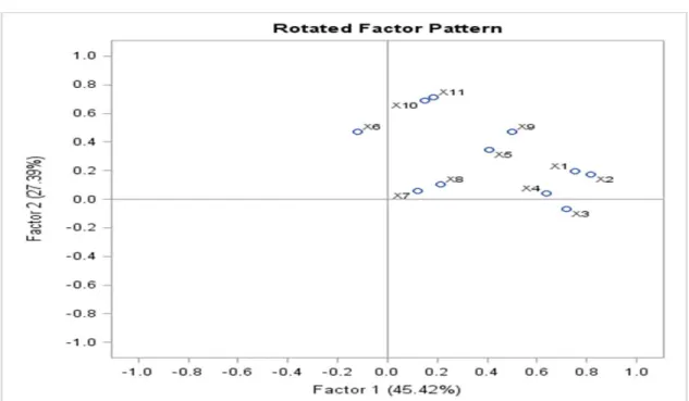
The factor pattern matrix as shown in table 5.1.2 displays the loadings for the solution with three factors. For interpretation purposes, we would take into consideration the loadings with absolute value greater than 0.5
Tabel 5.1.2. Factor Pattern Matrix
Factor1 Factor2 Factor3
x1 0.73599 -0.19750 -0.35499 x2 0.73108 -0.14725 -0.38324 x3 0.56163 0.006 -0.33489 x4 0.53514 0.07123 -0.19843 x5 0.62405 -0.05366 0.16444 x6 0.4054 0.16206 0.32069 x7 0.32966 0.78933 0.07770 x8 0.28121 0.78308 0.04620 x9 0.65677 -0.13014 0.11911 x10 0.41607 -0.16327 0.59865 x11 0.50419 -0.29296 0.47043
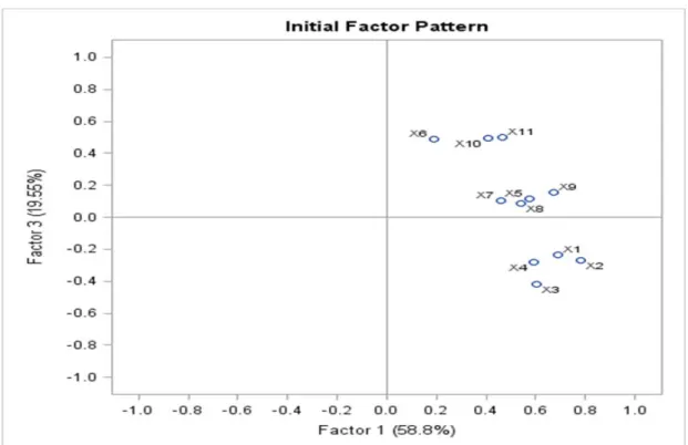
The initial factor extraction looks cleaner than the rotated factor patter as we don’t have variables representing different dimensions in the same factor and we need the factors to include the 11 variables in the analysis. Hence it is easier to name the factors.
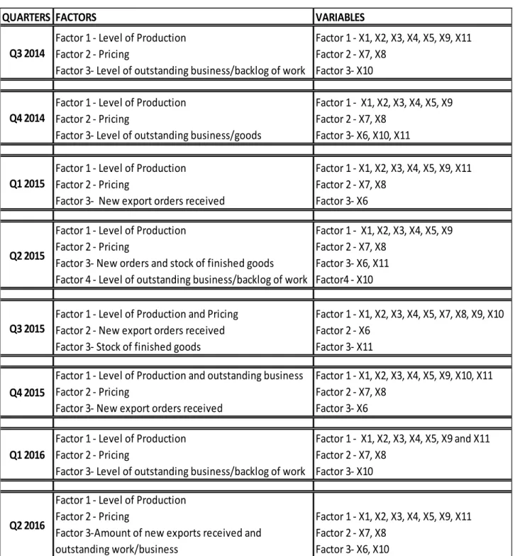
The first variable has a significant loading on factor 1. The other loadings on factor2 and factor3 are insignificant. Furthermore, the second variable has one significant loading on factor1 only and insignificant loadings on the other factors. The same pattern is evidenced in the third, fourth and fifth variable. Hence the general interpretation for the factor pattern is given as: Factor1: Loadings X1, X2, X3, X4, X5, X9 and X11. Factor2: Loadings X7 and X8. Factor3: Loadings X10.
From the factor extraction, and looking at the variable representations, we can assign unique characteristics to the factors as detailed below:
Factor2: Pricing.
Factor3: Level of outstanding/unfinished work
In order to establish the reliability, quality and internal consistency of these factors, we would test them using the Cronbach alpha.
The output for factor1 is shown in table 5.1.8 below. Recall that the minimum Cronbach alpha value we previously prescribed was 0.7. The raw alpha (0.764) and standardized alpha (0.723) for Factor1 are acceptable.
Tabel 5.1.3. Cronbach Alpha
Variables Alpha Variables Alpha
Raw 0.764364 Raw 0.67414
Standardized 0.762532 Standardized 0.67472
Factor 1 Factor 2
Consequently, the table of alpha for items deleted (Table 9.1.11) shows the correlation of each item together with its scale, the estimate of alpha if the variable were deleted from the analysis, and standardized correlation and alpha if deleted. Looking at the output, we see that no single variable stands out as helping the scale score more than other items. Notice that the alpha figures are all less than the overall Cronbach Alpha for Factor1. Hence Factor1 can be assumed to be reliable. The smallest value for alpha if deleted is for variable x1 (Production Level), which suggests that x1 contributes more to the overall alpha than other variables and without this variable, internal consistency would be reduced. This information is helpful in naming the factors. As stated earlier, factor 1 could be represented as ‘Level of Production’. The output for factor2 as below depicts the Conbach’s Alpha value for factor2 as 0.674 for raw alpha and 0.675 for standardized alpha. We could accept these values as it is significant to 0.7, which is the prescribed Cronbach alpha value. There is no Cronbach Alpha value for factor3 because the alpha option is not allowed with fewer than two variables.
5.2 Q4 2014
Just like the previous quarter, the data for Q4 2014 is suitable for Factor Analysis, because the overall data quality measure – KMO (see appendix) is approximetely 0.77 which is suitable.
From the eigenvalue‐one criterion, we would retain and interprete any component with an eigenvalue greater than the mean (in this case greater than one).
Tabel 5.2.1. Eigen values Matrix
Eigenvalue Difference Proportion Cumulative
1 3.50914459 2.21756 0.31900 0.319 2 1.29158657 0.12461912 0.11740 0.43640 3 1.16696745 0.1881656 0.10610 0.54250 4 0.97880184 0.10889727 0.08900 0.63150 5 0.86990458 0.10822003 0.07910 0.71060 6 0.76168454 0.11031297 0.06920 0.77980 7 0.65137157 0.07717284 0.05920 0.83900 8 0.57419873 0.05046785 0.05220 0.89120 9 0.52373088 0.13104561 0.04760 0.93890 10 0.39268527 0.11276129 0.03570 0.97460 11 0.27992398 0.02540 1 From the table 5.2.1, it is evident that the first, second and third factors have eigenvalues greater than 1 and hence would be retained. These factors account for 54.3% of the total variability of all the variables.
The scree plot of the eigenvalues and factors also guides in suggesting the the number of factors to be retained are the data points that are above the break (i.e point of inflexion).
The factor pattern matrix in table 5.2.2 displays the loadings for the solution with three factors. For interpretation purposes, we would take into consideration the loadings with absolute value greater than 0.5.
The initial factor extraction looks clean and we need the factors to include the 11 variables in the analysis. Hence we can name the factors.
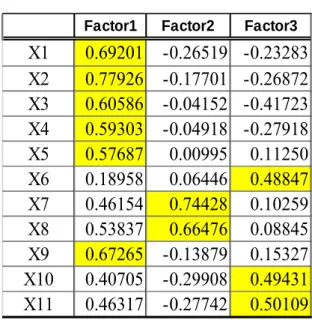
Tabel 5.2.2. Factor Pattern Matrix
Factor1 Factor2 Factor3
X1 0.69201 -0.26519 -0.23283 X2 0.77926 -0.17701 -0.26872 X3 0.60586 -0.04152 -0.41723 X4 0.59303 -0.04918 -0.27918 X5 0.57687 0.00995 0.11250 X6 0.18958 0.06446 0.48847 X7 0.46154 0.74428 0.10259 X8 0.53837 0.66476 0.08845 X9 0.67265 -0.13879 0.15327 X10 0.40705 -0.29908 0.49431 X11 0.46317 -0.27742 0.50109
From the table above, the variables with significant loadings on thefactors are outlined below:
Factor1: Loadings X1, X2, X3, X4, X5 and X9.
Factor2: Loadings X7 and X8.
Factor3: Loadings X6, X10 and X11.
From the factor extraction, and looking at the variable representations, we can assign unique characteristics to the factors as detailed below. Note that this is a similar trend to the preceeding quarter in 2014. Factor1: Level of production. Factor2: Pricing. Factor3: Level of outstanding business and goods To establish reliability, quality and internal consistency of these factors, we would test them using the Cronbach Alpha.
The output for factor1 is shown in table 5.2.3 below. The raw alpha (0.7680) and standardized alpha (0.777) for Factor1 are acceptable, since the minimum prescribed Cronbach Alpha value is 0.7.
Tabel 5.2.3. Cronbach Alpha
Variables Alpha Variables Alpha Variables Alpha
Raw 0.780036 Raw 0.72591 Raw 0.38403
Standardized 0.777434 Standardized 0.72602 Standardized 0.37201
Factor 1 Factor 2 Factor 3
The correlation of each item together with its scale, the estimate of alpha if the variable were deleted from the analysis, and standardized correlation and alpha if deleted, is shown in Table 9.2.11 (see appendix)
From the table, no single variable stands out as helping the scale score more than other items. The alpha figures are all less than the overall Cronbach Alpha for Factor1 and Factor1 can be assumed to be reliable. The smallest value for alpha if deleted is for variable x2 (Level of new customers or new business received). From Table 5.2.3, the Cronbach Alpha value for factor2 is 0.726 for raw alpha and 0.726 for standardized alpha, which is acceptable. Factor 3 is not reliable or consistent.
5.3 Q1 2015
The data from Q1 2015 is suitable as the KMO test shows a value of approximately 0.76. We are retaining and interpreting any component with an eigenvalue greater than the mean (in this case greater than one).From the table 5.3.1, we are retaining the first, second and third factors with eigenvalues greater than 1. These factors account for 54.4% of the total variabilty of all the variables.
Tabel 5.3.1. Eigen values Matrix
Eigenvalue Difference Proportion Cumulative
1 3.43498146 2.10284 0.31230 0.3123 2 1.33213727 0.11532435 0.12110 0.43340 3 1.21681293 0.24682531 0.11060 0.54400 4 0.96998762 0.14500352 0.08820 0.63220 5 0.8249841 0.04830169 0.07500 0.70720 6 0.77668241 0.10372895 0.07060 0.77780 7 0.67295347 0.04557585 0.06120 0.83900 8 0.62737762 0.10059504 0.05700 0.89600 9 0.52678258 0.10541977 0.04790 0.94390 10 0.42136281 0.22542506 0.03830 0.98220 11 0.19593775 0.01780 1 Consequently, from the scree plot of the eigenvalues and factors. The number of factors to be retained is the data points that are above the break. From the factor pattern matrix displayed in table 5.3.5, we see the loadings for the solution with three factors. As earlier stated, we would take into consideration the loadings with absolute value greater than 0.5.
The initial factor extraction looks clean and we can conclude on the factors to obtain.
Tabel 5.3.2. Factor Pattern Matrix
Factor 1 Factor 2 Factor 3
X1 0.76322 -0.05847 -0.40952 X2 0.78889 -0.08577 -0.38495 X3 0.56021 0.04703 -0.28618 X4 0.49436 -0.22995 -0.05059 X5 0.5842 -0.20342 0.04639 X6 0.18442 -0.12344 0.62385 X7 0.34798 0.7937 0.09209 X8 0.45201 0.7075 0.18560 X9 0.68222 -0.10018 0.19262 X10 0.46798 -0.18738 0.45415 X11 0.53551 -0.18438 0.37260
From the table above, the variables with significant loadings on thefactors are outlined below: Factor1: Loadings X1, X2, X3, X4, X5, X9 and X11 Factor2: Loadings X7 and X8. Factor3: Loadings X6. From the foregoing, we can assign unique characteristics to the factors as detailed below. Factor1: Level of production. Factor2: Pricing. Factor3: Amount of new exports received.
We would test them using the Cronbach Alpha in order to establish reliability, quality and internal consistency of these factors,
The output for factor1 is shown in table 5.3.3 below. The raw alpha (0.780) and standardized alpha (0.776) for Factor1 are acceptable, since the minimum acceptable Cronbach Alpha value is 0.7.
The Cronbach Alpha value for factor2 is 0.672 for raw alpha and 0.673for standardized alpha, which could be accepted.
Tabel 5.3.3. Cronbach Alpha
Variables Alpha Variables Alpha
Raw 0.780211 Raw 0.67197
Standardized 0.773593 Standardized 0.67285
Factor 1 Factor 2
The correlation of each item together with its scale, the estimate of alpha if the variable were deleted from the analysis, and standardized correlation and alpha if deleted, is shown in Table 9.3.11 (see appendix)
From the table, no single variable stands out as helping the scale score more than other items. The alpha figures are all less than the overall Cronbach Alpha for Factor1, hence can
be assumed to be reliable. The smallest value for alpha if deleted is for variable x2 (Level of new customers or new business received). The Cronbach alpha value for factor3 is not suitable.
5.4 Q2 2015
The data from Q4 2014 is also suitable for Factor Analysis as the overall data quality measure – KMO is suitable. Like previous quarters, we would retain and interprete any component with an eigenvalue greater than the mean (in this case greater than one), according to the eigenvalue‐one criterion as shown in Table 5.4.1Tabel 5.4.1. Eigen values Matrix
Eigenvalue Difference Proportion Cumulative
1 3.19215477 1.81012425 0.29020 0.2902 2 1.38203052 0.14137048 0.12560 0.41580 3 1.24066005 0.22527745 0.11280 0.52860 4 1.0153826 0.10566874 0.09230 0.62090 5 0.90971386 0.2300707 0.08270 0.70360 6 0.67964317 0.01560915 0.06180 0.76540 7 0.66403401 0.04029248 0.06040 0.82580 8 0.62374153 0.03851353 0.05670 0.88250 9 0.58522801 0.10631073 0.05320 0.93570 10 0.47891728 0.25042308 0.04350 0.97920 11 0.2284942 0.02080 1 The first, second, third and fourth factors have eigenvalues greater than 1 and hence would be retained. These factors account for 62.1% of the total variability of all the variables, the scree plot (see appendix) also explains this.
The factor pattern matrix shown in table 5.4.2 displays the loadings for the solution with three factors. For interpretation purposes, we would take into consideration the loadings with absolute value greater than 0.5.
The initial factor extraction looks clean and we need the factors to include the 11 variables in the analysis. Hence we can name the factors.
Tabel 5.4.2. Factor Pattern Matrix
Factor1 Factor2 Factor3 Factor4
X1 0.72283 -0.32822 -0.30893 0.21712 X2 0.74851 -0.2888 -0.31793 0.2226 X3 0.57588 0.13936 -0.36704 -0.155 X4 0.53816 -0.0523 -0.07729 -0.1287 X5 0.5778 -0.1561 0.22003 0.08317 X6 0.21917 0.11162 0.62728 0.57223 X7 0.44601 0.70258 -0.03475 0.09094 X8 0.3719 0.73123 0.02427 0.03713 X9 0.66483 -0.0365 0.16329 -0.0435 X10 0.41589 0.06866 0.26875 -0.7076 X11 0.39249 -0.3123 0.60072 -0.1776
Looking at Table 5.4.2 above, the variables with significant loadings on thefactors are outlined below: Factor1: Loadings X1, X2, X3, X4, X5 and X9. Factor2: Loadings X7 and X8. Factor3: Loadings X6 and X11. Factor4: Loadings X10 From the factor extraction, and looking at the variable representations, we can also assign unique characteristics to the factors as detailed below. Factor1: Level of production. Factor2: Pricing. Factor3: New orders and stock of finished goods Factor4: Level of outstanding business and goods To establish reliability, quality and internal consistency of these factors, we would test them using the Cronbach Alpha.
The output for factor1 is shown in table 5.2.3 below. The raw alpha (0.771) and standardized alpha (0.765) for Factor1 are acceptable.
Tabel 5.4.3. Cronbach Alpha
Variables Alpha Variables Alpha Variables Alpha
Raw 0.77074 Raw 0.65611 Raw 0.33591
Standardized 0.76474 Standardized 0.65644 Standardized 0.34178
Factor 1 Factor 2 Factor 3
The estimate of alpha if the variable were deleted from the analysis, and standardized correlation and alpha if deleted, is shown in Table 9.4.11 (see appendix).
No single variable stands out as helping the scale score more than other items. The alpha figures are all less than the overall Cronbach Alpha for Factor1 and can be assumed to be reliable. The smallest value for alpha if deleted is for variable x2 (Level of new customers or new business received).
Also, the Cronbach Alpha value for factor2 is approximately 0.656 for raw alpha and 0.656 for standardized alpha, which is also acceptable.
Factor 3 is incosistent since the cronbach alpha value is much lower than 0.7 as shown in Table 5.4.3. Cronbach alpha value for Factor 4 does not exist since it consists of one variable only.
5.5 Q3 2015
The data from Q3 2015 is suitable for Factor Analysis since the KMO is approximetely 0.800. (see appendix, table 9.5.2) According to the eigenvalue‐one criterion, we would retain and interprete any component with an eigenvalue greater than the mean.Tabel 5.5.1. Eigen values Matrix
Eigenvalue Difference Proportion Cumulative
1 3.46265276 2.29910406 0.31480 0.3148 2 1.16354869 0.11577519 0.10580 0.42060 3 1.0477735 0.10681919 0.09530 0.51580 4 0.94095431 0.08962205 0.08550 0.60140 5 0.85133227 0.12073843 0.07740 0.67880 6 0.73059384 0.0218302 0.06640 0.74520 7 0.70876364 0.00468899 0.06440 0.80960 8 0.70407465 0.09492568 0.06400 0.87360 9 0.60914897 0.05064057 0.05540 0.92900 10 0.5585084 0.33585943 0.05080 0.97980 11 0.22264897 0.02020 1 The Eigen values matrix in the table above shows that the first, second and third factors have eigenvalues greater than 1 and hence would be retained. These factors account for 52% of the total variability of all the variables.
Furthermore, the factor pattern matrix below displays the loadings for the solution with three factors. For interpretation purposes, we would take into consideration the loadings with absolute value greater than 0.5.
Tabel 5.5.2. Factor Pattern Matrix
Factor1 Factor2 Factor3
x1 0.74542 -0.01590 -0.49437 x2 0.75704 0.01653 -0.46990 x3 0.51088 -0.39929 -0.18567 x4 0.51593 -0.20976 0.11056 x5 0.51465 0.37172 0.13759 x6 0.31985 0.49373 0.33302 x7 0.51706 -0.45432 0.36055 x8 0.52969 -0.32305 0.49990 x9 0.63972 0.06338 0.05582 x10 0.49387 0.19485 0.13984 x11 0.05884 0.47423 0.49833 The general interpretation for the factor pattern is given as: Factor1: Loadings X1, X2, X3, X4, X5, X7, X8, X9 and X10.