Analysis of spinning reserves in systems with variable power sources

978-1-5386-1488-4/18/$31.00 ©2018 IEEE

Analysis of spinning reserves in systems with variable

power sources

P. M. Fonte

ISEL – Instituto Superior de Engenharia de Lisboa Instituto Politécnico de Lisboa

LCEC – Low Carbon Energy Conversion Lisbon, Portugal

pfonte@deea.isel.ipl.pt

1

_{Cláudio Monteiro}

1,2

_{Fernando Maciel Barbosa}

1_{University of Porto, Faculty of Engineering} 2_{INESC TEC}

Porto, Portugal cdm@fe.up.pt, fmb@fe.up.pt

Abstract— In this paper is studied an approach based on risk assessment to solve the scheduling of a power production system with variable power sources. The spinning reserves resulting from the unit commitment are analyzed too. In this methodology there are no infeasible solutions, only more or less costly solutions associated to the operation risks, such as, load or renewable

production curtailment. The uncertainty of forecasted

production and load demand are defined by probability distribution functions. The methodology is tested in a real case study, an island with high penetration of renewable power production. Finally, forecasted and measured reserves are compared, once the reserves are strongly linked with the forecasting quality. The results of a real case study are presented and discussed. They show the difficulty to achieve complete robust solutions.

Index Terms—Generation curtailment, probabilistic forecasting, risk assessment, uncertainty.

I. INTRODUCTION

The scheduling of production power systems is always a challenging task. If a significant part of production is based on renewable energy sources (RES), with high variability, the challenges increase even more. Insular power systems without connections to continental networks are a particular demanding case. Efficient and precise forecasting models can help to decrease the uncertainty associated with renewable power plants. On the other hand, a careful choice of the spinning reserves, can avoid stability problems in the network which could lead to generation curtailment, load shed or even blackouts.

There are several approaches to define the amount of reserves. In a deterministic point of view, the reserve can be defined as a given percentage of forecasted load, a percentage of renewable production forecasts, equal to the amount of the most loaded unit, (generally for the primary reserve) or a mix of some of the previous rules. In the case of probabilistic approach, it is calculated from the probability of not having enough generation to meet the load (due to load and production forecasting errors), or using approaches based on standard

deviation of load forecasting errors, among others [1],[2]. The reserves can be divided in upward and downward reserves each one with different roles. The first intends to answer to a loss of power production due to generation outages or forecasting errors (when the forecasted power production is higher than the real one or if the load forecasted is lower than the real one). The second is generally related to forecasting errors when the power production is higher than the predicted or the load is lower than the forecasted.

An approach widely used, to the scheduling with uncertainty, is the stochastic programming [3], chance-constrained [4] or robust optimization [5] with the uncertainty defined by different scenarios [7]. The drawback of the scenario-based is the high number of realizations to captures the probabilistic behavior of the uncertainty. The excessive time needed to solve all the scenarios is the major disadvantage, once the unit commitment (UC) and the economic dispatch (ED) are solved for each scheduling scenario.

Contrary to scenarios-based, in this work is proposed the estimation of risk using directly the probability density function of the random variables. With this approach, there are no infeasible solutions. Based on the trade-off between economic and reliability of the system, all solutions are accepted provided that the risk and consequent cost are acceptable.

The case study is based on the Portuguese Island of São Miguel (Azores). The final goal of this work is to show the applicability of the methodology, as well as to conclude about the capacity of the reserves to deal with the forecasting errors. In this work it is not considered a predefined value for the reserves; it will be defined dynamically from reliability and operational risk minimization.

II. RISK ASSESSMENT APPROACH

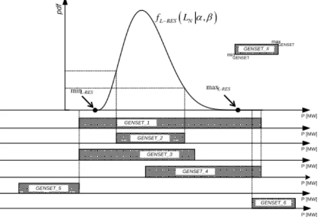
In Fig. 1 an example of the proposed risk assessment is depicted. The probability density function fL-RES represent the forecasted net load (LN) obtained by subtraction of the forecasted load by the forecasted renewable production (L-RES) [5],[8]-[10], and is defined by a Beta distribution

bounded by the limits of net load, minL-RES and maxL-RES. In other words (L-RES) represents the amount of power that must be produced by the thermal units. GENSET_# represents a generic thermal generation mix, whose limits are defined by

minGENSET and maxGENSET. Six different theoretical thermal generation mixes (GENSETs) are analyzed.

Figure 1. Example of risk assessment.

In the case of GENSET_1 it is verified that the minGENSET is lower than the minL-RES, which means that the probability of the GENSENT_1 work below the minimum generation capacity, is zero. On the other hand, the maxGENSET is higher than maxL-RES meaning that the mix has enough available power to feed the entire net load. The GENSET_2 shows a mix that do not have the capacity to feed all the range of net load. Exists some probability of load shed due to the lack of thermal power capacity and some probability of thermal units working below the minimum. In the case of GENSET_3, there is a probability of the net load to be higher than available production and, consequently, a certain probability of load shed to avoid blackouts. GENSET_4 shows the opposite case, the mix has enough power capacity to feed the maximum value of net load but, at same time, some probability of the thermal units work below the minimum. One option to decrease the probability of working below the minimum is the RES curtailment increasing

minL-RES in order to become higher than minGENSET or, at least, approximate the two values. The case of GENSET_5 the probability of load shed is one, meaning that GENSET does not have capacity to feed any net load. Finally, in the case of GENSET_6, the net load is so reduced, that the GENSET has a very high probability to work below the minimum, even with RES curtailment. Ideally, to each value of net load, the most convenient solution should be approximated by GENSET_1. However, it must be noticed that the set of possible thermal mixes are discrete and, consequently, cannot be possible to cover the entire net load necessities without load or wind curtailment.

Due to the uncertainty in load and renewable production forecast, generally, it is hard to find a completely robust/economic scheduling solution. In this sense, and for security, the scheduling is generally done in a conservative way, with low risk, but sometimes far away from an optimal operation. The system operator of the network under study, do

not use a fixed level of reserves. Instead, the reserves vary according to renewable production, time of day and even the experience of the system operators themselves.

III. DESCRIPTION OF THE METHODOLOGY

The proposed methodology is separated in 2 steps. The first one is the definition of the equivalent optimal generation unit.

A. Equivalent optimal generation unit

This procedure intends to create a database with all GENSET combinations and consists on a pre-processing procedure which is done only once (offline), being updated only if there is a change in the number or rated power of thermal units. In fig. 2 the procedure to create the database with equivalent optimal generation unit for each GENSET is shown.

Figure 2. Procedure to obtain the equivalent optimal generation unit (GENSET)

The proceeding starts with the definition of the mathematical expression for the fuel consumption of each thermal unit. The cost functions were defined as convex, continuous and second order. With the set of thermal units is created a dataset with all possible combinations of thermal units, defining each combination as GENSET with the respective maximum (maxGENSET) and minimum (minGENSET) limits of generation. To each GENSET is solved an ED for different values of load in order to define an equivalent generator. The problem’s restrictions were minimum and maximum production limits of each unit and the total production has to be equal to the load. Transmission losses were not taken into account. Calculation speed is the added value of this method. For each net load value is possible to calculate the power production that each unit must generate and, at the same time, the fuel consumption cost. Due to this, it is not necessary to run any ED during the on-line scheduling which will reduce the computation time. This procedure can appear to be exhaustive and time consuming, however is done only once and off-line. At the same time it is very dynamic. If there is an unavailable unit it’s enough to cut all GENSETs with that unit from the database.

p d f P [MW] P [MW] P [MW] P [MW] P [MW] P [MW]

L-RES maxL-RES

 ,  L RES N f L   GENSET_1 GENSET_2 GENSET_3 GENSET_5 GENSET_4 GENSET_6 P [MW] min GENSET_# max GENSET minGENSET

Determination of fuel consumption curves for each thermal unit

(with Specific Fuel Consumption)

Definition of all thermal units combinations (GENSET)

(Characterization of technical limits)

Database with optimal production

(each GENSET in function of net load)

Resolution of economic dispatch

B. Unit commitment based on risk assessment

In fig. 3, a diagram of the complete process for UC is shown. The complete formulation of this methodology can be found in [11].

Figure 3. Unit commitment based on risk assessment 1) Probabilistic forecasts

For each hour ahead, the load and RES production forecasts are received and aggregated as net load, which are the input of the algorithm. This process is deeply described in [8]. Very often, in this specific case study, during the off-peak periods with low load and high RES, the thermal units are forced to work below the technical minimum. To increase artificially the necessity of thermal production, the system operators choose to cut the wind production which demands a special care with the RES forecasting [12]. The measured data of RES production and load demand were provided by the system operator. The RES and load forecasts were provided by Smartwatt, Solutions

for Energy Systems (http://singular.smartwatt.net). 2) Evaluation of each GENSET

Following the example of Fig. 1, once the pdf of the net load for each hour ahead is known, a risk assessment for each GENSET is done calculating the risk (probability) of load shed, production below the minimum and the risk of normal operation. When there is a probability of production below the minimum, it is necessary to calculate the quantity of wind production that should be curtailed. In this case, there are two situations: the available wind production is lower than the curtailment need and the thermal units still work below the minimum, or the available wind production is higher than the curtailment necessity, being necessary to curtail only a percentage.

After the calculation of all risks for each hour ahead is mandatory to calculate the power associated to each risk. In (1)

1 ,

L RES h

F_ is the inverse of cumulative density function (cdf) of net load for each hour ahead h, prob(WC) is the risk of wind curtailment and

P

ˆ

_w is the forecasted wind generation.





1





,

ˆ

min

,

2

h L RES h w h

prob WC

P WC





_

F

_



_



_

P



_









(1)

Equation (2) calculates the thermal production below the minimum after total wind curtailment, where FL1H GEO h,



  is the

inverse of net load cdf with all wind production curtailed;

prob(min|WC) is the probability of production below the

minimum.





 









 

 

1 , 1 , 0 min min 2 min 0, 5 GENSET L H GEO h h GENSET L H GEO h prob WC P prob WC F F          











_

_

_

_





(2)

The load shed (LS) and thermal production within the limits (NO) are calculated by (3) and (4) respectively.

 

1

 

 

1 max 2 h L RES GENSET h h prob LS P LS F_





prob LS 











(3)





1 1

 





2 h h L RES h prob LS prob WC P NO F_



_

 



_





(4)

In order to conclude the evaluation of each GENSET, the costs related with each risk assessment are calculated. The risk cost of wind curtailment is calculated by (5) whereas the risk cost of load shed is done by (6),

 

 

, WC h h h WC C prob WC P WC C (5)

 

 

, LS h h h LS C prob LS P LS C . (6)

The parameters CWC and CLS are the wind curtailment and load shed cost, respectively, and are constants independently of the amount curtailed. After the total wind curtailment, if there is still a violation of the minimum limits of the GENSET, the risk cost is calculated by (7), where the cost CMIN_GEN is also considered constant.









minWC h, min h h MIN_GEN

C  prob WC 

P

prob WC C (7)

The cost of normal operation are calculated by (8), where

F[.] is the equivalent optimal generation unit consumption

function and CFUEL is the fuel cost.

 



 



 





 













, max min min min h h GENSET h NO h FUEL GENSET h GENSET h prob NO F E NO prob LS F C C prob WC F prob WC F         





























(8) Uncertainty aggregation (net load)

Evaluation of each GENSET

(Risk assessment and costs calculation) (Without start-up costs and contingencies)

Contingency analysis (N -1 thermal unit) Dynamic programming (Startup costs) Scheduling Probabilistic forecasts Load demand Renewable production Single period Multi period

For each hour h the total risk cost for a given GENSET based on risk assessment is given by (9).

, , min , ,

GENSET WC h LS h WC h NO h

C



C



C



C



C

(9)

The result of (9) is not a real costs, it is a risk costs calculated only to define the scheduling. The real costs should be calculated with the measured values.

3) Contingency analysis and dynamic programming

After, an (N-1) contingency analysis is done by (10) considering the outage of a single thermal unit whose failure cannot be repaired within this period. The process is done independently for each hour ahead (single period).









 







 



( 1), _ _ , _ 1 _ , _ _ 1 , 1

GENSET N h UNIT GENSET nS nB h

S GENSET n S nB h B GENSET nS n B h C n U C n U C n U C              (10)

If only one thermal unit is online, there is a risk of blackout whose cost is evaluated by (11) where CBO is the blackout cost. The contingency probability is defined by U, ns and nB are the number of units type GS and GB, respectively.







 



( 1), 1 , ,

GENSET N h GENSET h N LS h BO

C _  U C U E L C C

(11)

The start-up costs are integrated through a forward dynamic programming. To reduce the computation time the solutions of each period h are rearranged in ascending order. Only the solutions with costs that are inside of a threshold are tested. Thus, only solutions near the best solutions are tested at each state.

IV. CASE STUDY

The case study is based on the generation system of São Miguel Island, composed by the production sources depicted in table I. The unique thermal power plant is equipped with 4 units with 7,2 MW of rated power plus 4 with 16,5 MW. Thus 256 combinations of GENSETs are reduced to 24 GENSETs which lead to a more tractable problem. In table II the production limits of thermal units and the parameters of fuel consumption functions are shown.

TABLEI

RATED POWER FOR EACH POWER SOURCE

Source (#units) total power

Fuel 4 ₄ 28 MW _{64 MW}

Wind 9 9,4 MW

Small hydro 7 5 MW

Geothermal 5 29,6 MW

TABLEII

PARAMETERS OF THE THERMAL UNITS

Units Parameters Values

GS Pmin 3 848 kW Pmax 7 200 kW a 2,723e-6 g/kW2 b 0,112 g/kW c 120,96 g GB Pmin 8 410 kW Pmax 16 500 kW a 1,19e-6 g/kW2 b 0,105 g/kW c 311,85 g

The values of (5) up to (11) are shown in table III [13].

TABLEIII

PARAMETERS FOR THE CASE STUDY

Parameters Values

Cost Load shed €/MWh (CLS) 1800

Cost Wind curtailment €/MWh (CWC) 84

Cost Minimum violation €/MWh (CMIN_GEN) 157,5

Cost Fuel $/g (CFUEL) 0,0007

Probability Contingency % (U) 1,5

Cost Blackout € (CBO) 10 000

Cost Start-up GS € 455

Cost Start-up GB € 910

Threshold € 1000

In Fig. 4 the forecasted net load, with 90% of confidence is depicted, as well the GENSET limits of the committed units. The unit commitment is done to a 24 hours horizon and repeated for a 7 days period, between 0h00 of February 25th _up to 23h00 of March 3rd_{, 2014. The simulation of 168 hours took} 3,35 seconds on a laptop with an Intel Core i3 and 2,3 GHz processor.

Figure 4. Net load forecasting and resulted scheduling

In a first analysis, during the peak periods, the GENSET limits present a good coverage of the point forecast as well as the uncertainty, with exception of Mach 1st _{(after 18:00). In this} case, there is some risk of load shed, but the cost of a different GENSET is higher than the cost associated to the load shed. In the off-peak periods the situation is different once in several periods the limits of the chosen GENSET are within the limits of the net load uncertainty. This means that there is a risk of load shed and at same time wind curtailment or even production below the minimum. However, analyzing the costs, the chosen GENSET showed to be the cheapest one. There are cases where the point forecast is lower than the minimum of the GENSET, once it is more profitable to curtail the wind generation or produce below the minimum than choose another combination of thermal units. In fig. 5 the forecasted and measured values of net load are depicted.

Figure 5. Forecasted vs measured net load

0 10 20 30 40 50 Pow e r [MW ] Uncertainty Forecasted GENSET limits 0 10 20 30 40 50 Pow e r [M W ] Forecasted GENSET limits Measured

During several off-peak periods, the RES forecasted values were underestimated. The forecasting in these periods is demanding once the wind curtailment is not an explanatory variable for wind power forecasting. Even with accurate models remarking errors can be introduced. In figure 6 the forecasted and measured downward reserves are depicted.

Figure 6. Downward reserves

As consequence of underestimated RES production, there were negative downward reserves during several off-peak periods, leading to the necessity of wind curtailment or even units of GENSETs working below the minimum. In figure 7 the upward reserves are shown.

Figure 7. Upward reserves

In spite of the measured, reserves follow the forecasted ones. Occasionally there were some periods with negative reserves which reveal potential periods of load shedding. In tables IV and V the forecasted and measured reserve values are depicted.

TABLEIV

FORECASTED AND MEASURED RESERVES

Reserve Forecasted Measured

Upward 8,75 MW 9,80 MW

Downward 4,71 MW 3,66 MW

Due to the RES underestimation was expectable the increasing of average measured upward reserve and a decreasing of measured downward reserve.

TABLEV

FORECASTED AND MEASURED RESERVES

Load shedding

Wind

curtailment minimum Below

Forecasted 0 h 9 h 0 h

0 MWh 8,89 MWh 0 MWh

Measured 3 h 32 h 1 h

3,59 MWh 70,51 MWh 0,9 MWh

According with table V, without any action of the system operator, 3 hours and 3,66 MW of load shedding can occur. Nevertheless, it should be noticed that all the assessment was

done based on hourly average values whereby the dynamic within the hour was not considered. A deep analysis showed that this problem can be outperformed by the power plant operators, delaying some maneuvers or using the boost of the thermal units, since it was considered that the units start at the beginning of the hours and the starting time is neglected.

V. CONCLUSIONS

As conclusion, the proposed approach allows the implicitly determination of the reserves, because they are already incorporated in the uncertainty. If the system operator find some noticeable deviation, between the forecasted values and measured ones, it is very fast to run again the algorithm or reconfigure the available thermal solutions. The proposed algorithm can be a good alternative to those based on scenarios, broadly presented in literature. The computation time is reduced because it is not necessary to run an UC and ED to each scenario, once the processing time is a very important issue mainly when often refreshes are needed. Other important conclusion is that the success of the proposed method is deeply connected with the quality of the forecasts.

REFERENCES

[1] M. Doostizadeh, F. Aminifar, H. Ghasemi, and H. Lesani, “Energy and Reserve Scheduling under Wind Power Uncertainty: An Adjustable Interval Approach,” IEEE Trans. Smart Grid, vol. 7, no. 6, pp. 2943– 2952, 2016.

[2] R. J. Bessa et al., “Reserve Setting and Steady-State Security Assessment Using Wind Power Uncertainty Forecast: A Case Study,” IEEE Trans.

Sustain. Energy, vol. 3, no. 4, pp. 827–836, Oct. 2012.

[3] M. Di Somma, et al., "Stochastic optimal scheduling of distributed energy resources with renewables considering economic and environmental aspects", Renewable Energy, vol. 116, pp 272-287, Feb. 2018

[4] M. Di Somma, et al., "Optimal Bidding Strategy for a DER aggregator

in the Day-Ahead Market in the presence of demand flexibility",IEEE

Trans. on Industrial Electronics Apr. 2018

[5] D. Pozo and J. Contreras, “A Chance-Constrained Unit Commitment With an Security Criterion and Significant Wind Generation,” IEEE

Trans. Power Systems, vol. 28, no. 3, pp. 2842–2851, 2013.

[6] H. Chen, H. Li, R. Ye, and B. Luo, “Robust scheduling of power system with significant wind power penetration,” in Proc. Power and Energy

Society General Meeting, pp. 1–5, 2012.

[7] L. Wu, M. Shahidehpour, and Z. Li, “Comparison of Scenario-Based and Interval Optimization Approaches to Stochastic SCUC,” IEEE Trans.

Power Systems, vol. 27, no. 2, pp. 913–921, 2012.

[8] P. Fonte, B. Santos, C. Monteiro, J. Catalão, and F. P. Maciel Barbosa, “Renewable Power Forecast to Scheduling of Thermal Units,” in Proc.

DoCEIS’13 - Doctoral Conference on Computing, Electrical and Industrial Systems, 2014.

[9] G. Liu and K. Tomsovic, “Quantifying Spinning Reserve in Systems With Significant Wind Power Penetration,” IEEE Trans. Power Systems, vol. 27, no. 4, pp. 2385–2393, 2012.

[10] A. Kalantari, J. F. Restrepo, and F. D. Galiana, “Security-Constrained Unit Commitment With Uncertain Wind Generation : The Loadability Set Approach,” vol. 28, no. 2, pp. 1787–1796, 2013.

[11] P. M. Fonte, C. Monteiro, and F. M. Barbosa, “Unit commitment based on risk assessment to systems with variable power sources", in Proc. 42nd Conference of the Industrial Electronics Society, pp. 3924–3929, 2016.

[12] P. M. Fonte and C. Monteiro, and F. M. Barbosa, “Net load forecasting in presence of renewable power curtailment,” Int. Conf. Eur. Energy

Mark. EEM, pp. 1–5, Jul. 2016.

[13] M. Parness, “The Environmental and Cost Impacts of Vehicle Electrification in the Azores,”, Msc. dissertation, Engineering Systems Division. M.I.T., 2011. -5 0 5 10 15 20 Pow e r [MW ] Forecasted Measured -5 0 5 10 15 20 25 Pow e r [MW ] Forecasted Measured