ii
GIS-BASED ANALYSIS OF SOCIO-ECONOMIC
VARIATION IN ACCESSIBILITY TO GREEN SPACES
IN BARCELONA, SPAIN
ii
GIS-BASED ANALYSIS OF SOCIO-ECONOMIC
VARIATION IN ACCESSIBILITY TO GREEN SPACES IN
BARCELONA, SPAIN
Dissertation supervised by
Pedro Cabral, PhD
Professor at NOVA, Information Management School Universidade Nova de Lisboa, Lisbon, Portugal
Dissertation co-supervised by
Marco Painho, PhD
Professor at NOVA, Information Management School Universidade Nova de Lisboa, Lisbon, Portugal
Ignacio Guerrero, PhD
External professor at Universitat Jaume I Universitat Jaume I, Castellón de la Plana, Spain
iii
ACKNOWLEDGEMENTS
I want to thank my family as well as my supervisor and co-supervisors for their help and support.
iv
ANALYSIS OF SOCIO-ECONOMIC VARIATION IN
ACCESSIBILITY TO GREEN SPACES IN BARCELONA,
SPAIN, A GIS-BASED ANALYSIS
ABSTRACT
Accessibility to different services in cities has been studied as form of analysing equity, especially in urban settings. Green spaces are one of these services; they have known benefits on the wellbeing of the urban residents. This work intends to determine if the variation in accessibility to urban green spaces is affected by the distribution of socio-economic variables such as income, and how these affect the green equity in a city. Green spaces have been categorised into different functional levels based on their size and accessibility and equity has been analysed, taking into consideration income, density, migrant populations and age-based variables. The analysis conducted involved a network-based service area analysis as well as spatial and statistical analysis using ArcGIS, GeoDa and R. The case study selected was the city of Barcelona (Spain). The results of the analysis reject the hypothesis of inequity in accessibility at functional levels based on the variables studied although some spatial associations exist.
v
KEY WORDS
Accessibility Equity
Geographical information systems Hierarchical green spaces
Local Indicators of Spatial Association Network analysis
Socio-economic variation Spatial statistics
vi
ACRONYMS
EEA – European Economic Area
ESRI – Environmental Systems Research Institute GIS – Geographical Information Systems
LISA – Local Indicators of Spatial Autocorrelation MAUP – Modifiable Area Unit Problem
vii
INDEX
ACKNOWLEDGEMENTS ... iii ABSTRACT ...iv KEY WORDS ... v ACRONYMS ...vi INDEX ... viiINDEX OF TABLES ... viii
INDEX OF FIGURES ... ix 1. Introduction ... 1 1.1 Motivation ... 1 1.2 Background ... 1 2. Methodology ... 5 2.2 Methodological process ... 5
2.3 Study area and data ... 6
2.4 Categorisation of urban green spaces ... 12
2.5 Assessing accessibility ... 14
2.6 Spatial analysis ... 18
3. Results and discussion ... 21
3.1 Accessibility and distribution of green spaces ... 21
3.2 Socio-economic characteristics ... 28
3.3 Spatial autocorrelation ... 31
3.4 Equity ... 35
4. Conclusions ... 38
viii
INDEX OF TABLES
Table 2.1 Socio-economic variables. 10 Table 2.2 Minimum standards for urban green spaces 13 Table 2.3 Hierarchical classification of urban green spaces for Barcelona 13 Table 3.1 Man-Whitney U analysis of park access equity 36
ix
INDEX OF FIGURES
Figure 2.1 Methodology flow 6
Figure 2.2 Location of Barcelona 7 Figure 2.3 Districts and neighbourhoods of Barcelona 8 Figure 2.4 Network dataset for Barcelona and surrounding areas 11 Figure 2.5 Green spaces in Barcelona by categories 14 Figure 2.6 Difference between buffer-based and network-based service areas 15 Figure 2.7 Example of access points as facilities for service area analysis 17 Figure 2.8 Example of finished service areas 18 Figure 3.1a Service areas for residential parks 23 Figure 3.1b Percentage of total area covered for residential parks 23 Figure 3.2a Service areas for neighbourhood parks 24 Figure 3.2b Percentage of total area covered for neighbourhood parks 24 Figure 3.3a Service areas for quarter parks 25 Figure 3.3b Percentage of total area covered for quarter parks 25 Figure 3.4a Service areas for district parks 26 Figure 3.4b Percentage of total area covered for district parks 26 Figure 3.5a Service area for city parks 27 Figure 3.5b Percentage of total area covered for city parks 27 Figure 3.6 Maps depicting income, population density and percentage of migrant
population (2014) 29
Figure 3.7 Maps depicting percentages of population younger than 15, older than 60 and buildings built before 1960 (2014) 30 Figure 3.8 High and low LISA values 33
1
1. Introduction
1.1 Motivation
Urban green spaces play an important role in the improvement of the quality of life of urban residents, and the effects they have on health and wellbeing are well known Modern, densely populated, cosmopolitan cities in developed countries are constantly enacting policies to reduce inequalities in urban provision between districts and neighbourhoods, some of which may have historically congregated people with different socio-economic backgrounds. The common assumption usually is that lower-income neighbourhoods have a worse distribution in urban provisions than better off areas is prevalent, especially in large cities where immigration from less developed countries has also been prevalent, given that migrants tend to converge in more affordable districts. Distribution and accessibility to healthcare, education centres, social services and other type of similar urban services have occupied a great part of the concern of both residents and planners, and green spaces should not be left behind in this concern. If inequality in this realm exists, it is in the interest of all to act on those inequalities, finding ways of reducing them.
This work is particularly interested in analysing if such inequality exists, by means of trying to find possible correlations between the accessibility to urban green areas in the city of Barcelona and the distribution of socio-economic factors such as income and migration.
1.2 Background
The study of urban equity and the development of policies to fight inequality in urban spaces is a common theme of study in the realm of urban geography and planning. In the context of urban settings and city planning equity refers to a state of fairness, where everyone is able to benefit from the services and advantages that derive from living in cities (“Urban Equity in Development”; 2014). These services can be of very different types and they cover a variety of needs that the urban populace might require; social services, transportation (Litman; 2002), education and healthcare, among others, as it is believed that the difference in accessibility to different services and activities has a measurable effect in the economic and social opportunities of the urban residents (Wang & Chen; 2015).
2
An important element considered when studying the equity in urban services is the accessibility to green spaces. A good and balanced distribution of green locations across the urban area that allows for improved accessibility to parks and green areas in general has become an important concern for policy-makers and urban planners (Xiao et al.; 2017). The interest lies in determining the equity in accessibility to green spaces, knowing the benefits that they provide to city inhabitants.
Green spaces and equity
There are evident short and long-term advantages in the presence of green spaces in urban areas, especially when aimed at improving the wellbeing of urban residents (Byrne et al. 2009). Research seems to indicate that the presence of accessible green spaces has numerous advantages, including increasing the propensity of engaging in physical activity (Hillsdon et al. 2006). The quality of life in an urban area is often linked to the presence of accessible green spaces for its residents, as green spaces are often the only contact many urban dwellers have with natural or semi-natural environments (Jorgensen et al. 2002),
The analysis of the possible effect of various socio-economic variables such as the ones described on the spatial distribution of services, particularly in cities and urban regions, is already a present research topic on the field, and has been studied in the past by authors like Nicholls (2001). The concepts of green equity, environmental equity and environmental justice are frequently used to express the need of finding inequalities in the distribution and access of green spaces in urban areas, especially when caused by socio-economic reasons such as ethnic or racial origin, or economic class (Taylor et al. 2006; Byrne et al. 2009). This concern has also extended to regulatory bodies; the European Environmental Agency (EEA) recommends that every urban resident should have a green space within 15 minutes of their residence (Barbosa et al. 2007).
Accessibility
The concept of accessibility and its role in respect to services within urban regions has been tackled by various authors and it is often a central concept in the realm of urban geography and planning (Xiao et al. 2017). Accessibility is traditionally defined as “the quality or characteristic of something that makes it possible to approach, enter or use it” (Cambridge Dictionary, 2016). Using this definition, we can understand accessibility in our context of study as the quality that a certain urban service has that enables it to be
3
approached. Urban green services hold that position as services and their accessibility determines how easily, or difficultly, it is to get access to them from any given point in the urban network. It is important to remark however, that the notion of what is considered “accessible” in a city and the parameters that account to that accessibility is quite complex (Talen, 1997).
Generally speaking, literature on the topic usually considers different approaches to assess the accessibility of green areas in a city or urban area (Talen and Anselin, 1998). One methodology frequently used is the “container” approach, which considers the total number of green areas and parks, either as an individual count or as a total area, within a single container unit, usually administrative divisions such as districts or census units. As a result, it is possible to determine which units have larger amounts of total green area when compared to their neighbours. Talen and Anselin (1998) consider however that results based on this approach could be inaccurate, given that the access to a green area in each unit is not limited to the population residing in the unit itself. This methodology would thus ignore the potential mobility of people from other units (Nicholls, 2001). The container method also suffers from the Modifiable Areal Unit Problem (MAUP), a well-known spatial analysis problem (Zhang et al. 2011), which is “the sensitivity of analytical results to the definition of units for which data are collected” (Fotheringham and Wong, 1990), referring to the fact that the measures taken are directly dependent on the spatial scale of the unit of analysis. Given that these units are generally chosen or defined arbitrarily (Jelinski and Wu, 1996), the spatial accessibility of a given service (parks, for example) may change depending on the size of the geographic container (Zhang et al. 2011). Smaller neighbourhoods or city districts, for example, would be affected by this when compared to their larger counterparts.
Another common strategy is the one known as the travel-cost approach, which measures the traveling distance from the administrative unit – generally its centroid – to a green space (Talen and Anselin, 1998), looking for the minimum travel distance, either in length or in time, to the nearest park (Zhang et al. 2011). Traditionally direct, Euclidean, distances are used to measure how accessible a unit is to a park, and while this seems intuitive on paper, it has as a main problem that it does not take into consideration real life barriers between two points, and the fact that people cannot move in a straight line through space, which might lead to inaccurate results (Nicholls, 2001; Xiao et al. 2017). Alternative approaches using short-path algorithms are commonly used and seem more
4
appropriate (Talen, 1997). A problem also frequently mentioned with this approach is the fact that people do not necessarily go to the green area that is the closest to their vicinity (Zhang et al. 2011). This issue is often addressed by measuring accessibility to different hierarchical levels of green areas, classifying them, for example, by size.
A variation of the previous approach exists with the “radius” method, in which service areas are calculated from each one of the green areas (instead of towards it), in which residents of a neighbourhood unit are considered to have accessibility to a particular green area if they are covered by its service area. This approach is often mentioned as the covering model of accessibility (Hodgart, 1978; Nicholls, 2001). This approach however suffers from a similar problem as the one already mentioned with the travel-cost approach; the radius is generally a buffer generated considering a determinate Euclidean distance, thus creating a perfect circle around the park or green area, which tends to provide an inaccurate representation of how people move through the urban fabric. Nicholls (2001) also identifies another problem; with the origin of the service area being located in the centroid of the park, it is assumed that the green area can be accessed from any point around it, which is not usually the case, which may lead to an overestimation in the results. Also, as the area of the green space increases, so does the distance between its centroid and the outer limit of the park, possibly causing an underestimation of what would be the real service of the green area (Nicholls, 2001).
This work implements this covering model of accessibility using network-based service areas instead of the traditional Euclidean-based buffers, using the solution proposed by Nicholls (2001) of using various entry points for each park as starting points of the service areas, with the objective of avoiding both over and underestimations. In order to address the fact that residents of a unit do not necessarily move exclusively to their nearest green area, a hierarchical classification of the green spaces is presented, using an adapted version of the green park classification presented by Van Herzele and Wiedemann (2003), which classifies the urban green areas by size-based categories, giving each category a fixed maximum distance of accessibility, which refers to the maximum distance residents are usually willing to move to access a park of a given rank (Van Herzele and Wiedemann, 2003).
5
2. Methodology
The methodology that follows describes the objectives and the research question of this work. In addition, it details the process followed in order to achieve the objectives and arriving to a meaningful conclusion.
2.1 Objectives
Main objective
1. Analyse if the variation in accessibility to urban green spaces in different
hierarchical categories has any correlations or is specially affected by the distribution of higher and lower income neighbourhoods, using as case study the city of Barcelona (Spain).
Secondary objectives
2. Analyse if there is a positive correlation between accessibility and other
socio-economic variables such as population density, migrant populations and age.
3. Determine if there is equity in access to urban green spaces based on the
socio-economic variables studied.
This work, by the means of the aforementioned objectives, attempts to answer specific
research questions, which are formulated in the following manner:
Do higher income neighbourhoods have a better access to urban green spaces than lower income neighbourhoods? How does income affect the distribution of spatial accessibility to urban green spaces?
Are there any other relevant socio-economic variables that play a role in this accessibility?
2.2 Methodological process
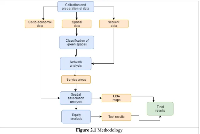
The intention is to analyse the accessibility to urban green spaces for each hierarchical level and then analysing how the selected socio-economic variables correlate with the distribution of the accessible areas. Thus, the methodology followed in this research can be divided into three sections. First, the accessibility to each green area in each hierarchical level is determined by the means of network-based service areas; this initial step is useful for drawing a first image of how the accessibility is distributed within the city in respect to the distribution of our variables. The Network Analyst tool available in ESRI’s ArcMap (version 10.4.1) was used with this intention. Following this, we look for
6
spatial correlations between the areas with high and low accessibility and areas where each one of the studied variables are present in high or low numbers. This is performed conducting tests searching for local indicators of spatial autocorrelation (LISA) using the GeoDa software (version 1.6.7).
Finally, we look for statistical correlations between accessibility and each one of the variables by conducting the Mann-Whitney U test using the R language. This step helps us determine whether or not there is indeed statistical evidence for correlations between the spatial distributions of each variable and the areas with high and low accessibility to green spaces. Using the information gathered from the three main steps results are presented and conclusions are drawn. Figure 2.1 displays the process of the methodology.
Figure 2.1 Methodology
2.3 Study area and data
This research has selected as a study area the city of Barcelona, the second largest city of Spain and the capital and most populous city of the autonomous community of Catalonia. Geographically, it is located by the Mediterranean Sea in the eastern coast of the Iberian Peninsula of Europe, as depicted in figure 2.2. The city is located between the Llobregat and Besòs rivers. It is located mostly on a plain between the two rivers, the Mediterranean Sea and the Collserola mountain range (Barcelona city portal, 2016). The Barcelona metropolitan area extends over the limits of the city proper with a population of around
7
4.7 million people in the total urban area (Demographia, 2016) and over 5 million in the total metropolitan area; this research however focuses only in the administrative unit that refers to the city proper, which is known as municipality of Barcelona.
Figure 2.2 Location of Barcelona
The municipality of Barcelona is the second most populous municipality in Spain and it is the core of one of Europe’s most populous metropolitan regions. This city was selected as the study case of this research due to its position as a large European metropolis, where the distribution of income and other socio-economic factors can be more evident. Being the second largest city of the country and with an important variation in density and overall socio-economic distribution (as it is displayed in the following sections), we consider Barcelona to be an interesting setting for this research.
8
The municipality of Barcelona occupies an area of around 102.2 km2 (Barcelona city
portal; 2016), which is about 10,220 ha. From an administrative standpoint, it is divided into ten districts and seventy-three neighbourhoods (Barcelona City Hall, 2016). This administrative division is displayed in the figure 2.3. The Department of Statistics of the city (Departament d’Estadística) collects, manages and distributes local and regional statistics at different administrative level; the most common are levels are district and neighbourhood.
This research works at neighbourhood-level, mainly due to the availability of data; while smaller administrative units do exist (such as census blocks), the availability of data at this level is rather limited, in some cases – income, for instance – due to privacy concerns. However, given the size of the city and the number and size of the neighbourhoods, they have been deemed appropriate for this research.
Figure 2.2 Districts and neighbourhoods of Barcelona. Note: Only districts are labelled.
The data used on this study has been collected from multiple sources, although an attempt has been made at using open data when possible, in order to make the methodology easily
9
replicable in other urban areas. The data used in this research included various vector shapefiles and network datasets (spatial data) as well as statistical data detailing information about the socio-economic aspects and settings of the city. The specifics about the origin and nature of the data used are explained hereunder.
Socio-economic data
This research uses local statistical data to determine the socio-economic characteristics of the city at neighbourhood level. As it has been mentioned earlier, neighbourhoods are the second administrative unit in a municipality after the districts, and data involving these units are usually readily available at the city hall and regional government websites. In the case of his research about Barcelona, the following data was used: population density, income, migrant population, population under 15 and over 60 and buildings built before 1960. This information was collected from the statistical data display tool available at the Department of Statistics website, managed by the city of Barcelona (Department of Statistics of Barcelona, 2016). The tool allows for the display of numerous types of data in tabular form, which could later be exported in CSV format.
The data selected was from the year 2014 and at neighbourhood level in all cases. Although later data was available for some of the categories, the latest for income was that of the year 2014 at the time of conducting the research, and being income one of the central pieces of the research and wanting to use data from a same year to avoid possible variations between the categories, that year was selected for the whole research. Also, some data – particularly that collected by means of the local census – was available at census area level, which is lower than neighbourhood and could provide a better spatial definition. However, not all data was available at this scale and once again for the sake of uniformity all data was collected at neighbourhood level.
Data Units
Demographic characteristics
Population density Inhabitants / km2
Migrant population Percentage of the total population
Population under 15 Percentage of the total population
Population over 60 Percentage of the total population
10
Income Income by family unit;
city average (%) = 100
Other
Buildings built before 1960 Percentage of the total
Table 2.1 Socio-economic variables
The main rationale behind the data picked for this research was selecting variables that could draw a picture of the socio-economic characteristics of the population living in each neighbourhood, taking into consideration different factors. On one hand, income is decidedly seen as one of the main social and economic indicators that can be used to explain inequity, particularly when talking about spatial distribution of services. Population density was considered a standard variable to take into account, given its expected impact on the distribution of public services like parks. The research also includes percentage of migrant population and percentage of the population younger than 15 and older than 60, as they are common variables in this type of research (Nicholls, 2001; Xiao et al. 2017). Older populations generally benefit from having accessible green spaces closer to where they live due to their reduced mobility, while children – who often depend on their parents for mobility – tend to primarily visit green spaces closer to their homes (Hillman et al. 1990; Van Herzele and Wiedemann, 2003). Thus, and given that we are working with green spaces hierarchically categorised by size, knowing how accessible the different green spaces are to this populations was considered interesting, from a research perspective.
Spatial data
Much of this research relies on the results of a network analysis conducted on spatial data. The details of this analysis are explained in the sections below, while this section refers to the spatial data that was used and the origin of said data. Vector data representing the city limits at municipal and neighbourhood level was obtained from the Cartographic and Geologic Institute of Catalonia and from the Barcelona municipal geoportal, which provided the spatial data in SHP format. In addition, shapefiles containing all green areas in the city of Barcelona as well as some other spatial data were extracted from Open Street Map using the online tool Mapzen. The green area vector file from Open Street Map proved to be more complete than the one available in the city geoportal, which only included major parks.
11
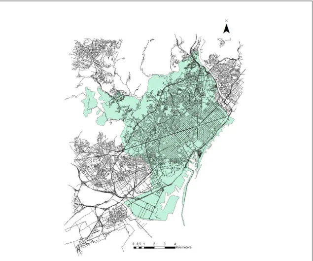
In order to conduct a network analysis that could assess accessibility, a network dataset was necessary. Network analysis relies on the use of a network-type layer that contains within it data about spatial movement, as well as spatial topologies. This allows for analyses that take into consideration physical impediments that might exist. Thus, a regular line shapefile displaying the roads – as they are commonly used on spatial analyses – would not be useful for this particular type of analysis.
Figure 2.4 Network dataset for Barcelona and surrounding areas.
Very precise and accurate network datasets are difficult to come by, and there are many companies that specialise in providing this type of data. This research opted for an open alternative, extracting and building a network dataset from an OSM file coming from Open Street Map. The network dataset was extracted and built using the ArcGIS Editor extension for ArcMap, resulting in a complete road network dataset compatible with the Network Analyst extension, as depicted in figure 2.4.
The shapefiles, network datasets and all spatial features used on this research were all transformed into a projected coordinate system, specifically the WGS 1984 Universal
12
Transversal Mercator (Zone 31N). Projected coordinate systems are preferred when performing this type of analyses, which rely heavily on distances and areas.
2.4 Categorisation of urban green spaces
Hierarchical categorisation
Urban green spaces are usually distributed unevenly across cities and large urban areas, and they can be very heterogeneous in nature and, particularly, in use. Thus, green spaces can have different functional levels, and any given park or green space in a city does not necessarily function as a substitute of any other, as different green spaces fulfil different functions (Van Herzele and Wiedemann, 2003). It has been suggested that different types of urban green spaces can be classified into categories taking into consideration particular typologies (Dunnett et al. 2002). These different “levels” of parks and green spaces are often classified hierarchically, and they tend to complement each other (Gupta et al. 2016).
These categorisations, especially when in the context of accessibility, take into consideration two main variables; the size of the space generally measured by area, and the effort that would take to access that park, measured either in distance or time. It is generally accepted that the larger (or better equipped) a green space is, the biggest the distance people may be willing to move to reach it (Van Herzele and Wiedemann, 2003). This type of direct relation between quality/size and distance is not unique to green spaces and it is usually also present in other forms of urban services.
This relation between distance and size of the green area can be observed in different scenarios. Parks of smaller size may be considered as acceptable spaces in crowded city centres and dense residential areas and residents are willing to move smaller distances to access parks of this type. Better equipped parks, which may be bigger in area, will attract residents even when located at the fringes of urban areas (Van Herzele and Wiedemann, 2003). This hierarchical categorisation is not universal however, and different places have created or adapted different categories – with different minimum sizes and maximum distances – according to the characteristics of their local region (Gupta et al. 2016). The distance people may be willing to move and the size of the park that they consider as acceptable for that distance will not be the same in an American urban setting – where extensive urban sprawling is common – and in a more compact and pedestrian-friendly European city.
13
Different authors have suggested different classification systems designed for different regions, such as Harrison et al. (1995), whose classification would become the basis for the British Accessible Natural Green Space Standards or the classification used by Oh and Jeong (2007) for his park accessibility analysis in Seoul. Van Herzele and Wiedemann (2003) present general standards for hierarchical park classification. This classification is shown in the table 2.2.
Functional level Maximum distance (m) Minimum surface (ha)
Residential green 150 Neighbourhood green 400 1 Quarter green 800 10 District green 1600 30 City green 3200 60 Urban forest 5000 >200
Table 2.2 Minimum standards for urban green spaces (Van Herzele and Wiedemann,
2003)
In this work the presented classification by Van Herzele and Wiedemann has been slightly modified to adapt it to the city of Barcelona, which follows the pattern of Spanish cities of being quite compact, especially when compared to other similarly large cities in the continent. We have decided for this work to include a minimum surface for what the aforementioned authors have named “residential green”, providing a minimum surface of 0.1 ha, resulting in the classification displayed in table 2.3
Functional level Maximum distance (m) Minimum surface (ha)
Residential green 150 0.1
Neighbourhood green 400 1
Quarter green 800 5
District green 1600 30
City green 3200 >60
Table 2.3 Hierarchical classification of urban green spaces for Barcelona
In the context of this research, we considered urban green spaces as all those publicly accessible green areas, which included all parks and public gardens as well as plazas located within the municipality. Urban forests and green pleasances (smaller than 0.1 ha) were not included, neither have been included linear green spaces (closed gardens across avenues or streets), and green areas of limited or impossible access (private gardens, green spaces between motorways and roundabouts).
14 Organising and classifying green spaces
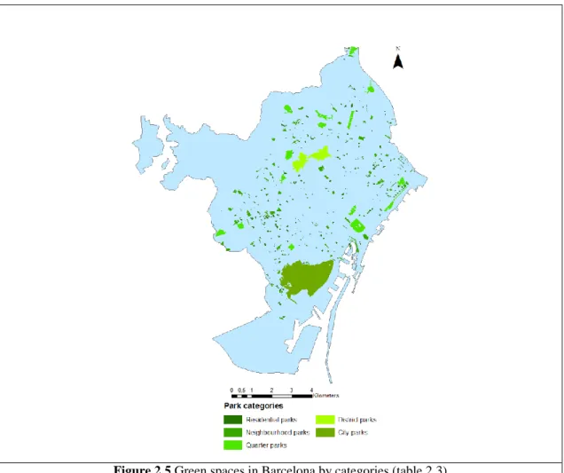
Spatial data in the form of shapefiles representing every green space in the city of Barcelona was downloaded from Open Street Map. The initial shape file was seriously disorganised as it included built areas and inaccessible areas – such as green fields near motorways or in the middle of roundabouts. In addition, many parks across the city were divided into several smaller shapefiles, which would cause inaccuracies when classified hierarchically if counted by themselves. The shapefile was then cleaned manually, removing all non-green areas, as well as areas that were meant to be included on this research (figure 2.5). After that, areas were calculated for each green space and each one was given a category from ‘A’ through ‘E’ depending on its size.
Figure 2.5 Green spaces in Barcelona by categories (table 2.3)
2.5 Assessing accessibility
This research has attempted to determine which areas of the city are more or less accessible to green spaces at each one of the functional levels described in table 2.3. Given that the ultimate intention is to assess whether or not there is a spatial correlation between areas considered of “high” and “low” accessibility with the spatial distribution of
15
variables such as income, it was decided to implement the covering model of accessibility (Hodgart, 1978) with the suggestions described by Nicholls (2001). This model asserts that areas within the city can be considered to have an adequate accessibility to a park if they are located within the service area of said park. From a network analysis perspective, a service area is the region that includes within it all streets that are accessible from a given point in space (“Service area analysis”, 2016). The service area is then the area that can be accessed from a certain point, taking into consideration parameters such as distance or time, as well as any physical barriers or limitations that may exist and that could limit the accessibility.
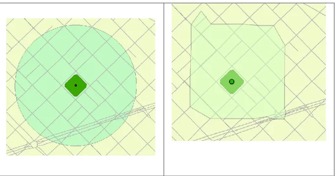
The covering model of accessibility originally contemplates a radius methodology (Hodgart, 1978), where a Euclidean distance is calculated from a central point – located generally in the centroid of the park – and a geometrical buffer is created around it (a Euclidean-based service area). As it has been detailed in the introductory section of this work, this methodology – as many similar others – assume the ability of moving in a straight line towards the park, and this is almost never the case given the existence of the urban fabric. The disadvantages presented by this implementation are solved by generating a network-based service area instead, that is a service area that takes into consideration the street network surrounding the starting point (Nicholls, 2001). Figure 2.6 depicts these differences. This is performed by ArcMap’s Network Analyst by using a shortest-path algorithm.
16
The service areas are generated using ArcMap’s Network Analyst tool. This tool requires a network dataset, which is a representation of a street network but that differs from a typical line or polygon shapefile displaying streets in the sense that it also stores and displays information about connectivity (“What is a network dataset?”, 2016). This means that besides displaying information about streets and physical barriers (normally in the form of points and polylines), the dataset also includes data about how the network is connected, the impediments and physical barriers that exist, as well as any other form of movement limitations.
Network datasets are not necessarily readily available and in many cases proprietary datasets can be acquired from companies that specialise in producing them. Open source alternatives do exist however, and as in with the green space data, Open Street Map was used on this work to acquire a network dataset for the city of Barcelona. Network datasets need to be extracted and built by the ArcMap software, thus the ArcGIS Editor for Open Street Map is a useful tool for extracting and analysing Open Street Map data, which is generally stored in .OSM format. The tool is integrated into the ArcMap interface and find, download and create OSM network datasets compatible with the Network Analyst tool.
The starting point whence the service area originates is called a “facility” by the network analyst tool. It is common in service area analyses that originate in areas (as opposed to lines or points) to place the facility on the centroid of the polygon, which can be calculated by the GIS software. It has been mentioned earlier that this implementation may lead to underestimations of the served area when dealing with large green spaces, due to the fact that the distance between the centroid and the boundaries of the green space will be included in the total distance. This can be solved by placing the facilities on the “access points” (Nicholls, 2001), which can be the intersections of incoming streets and the park boundary as shown in figure 2.7. This effectively minimises the service area underestimation problem. Each green space would include a series of entry points which would generate different, independent service areas; each service area would cover the area that is the most accessible to that access point in particular.
17
Figure 2.7 Example of access points marked as facilities for the service area analysis
The service areas are then generated using the “New service area” option in the network analyst tool. The creation of a service area requires the definition of certain parameters that will determine the layer properties of the output. The access points as defined earlier are selected as facilities, which means each point will generate a service area. Some impediments need to be defined for the generation of these areas, namely a length impediment measured in metres is selected. Given the objectives of analysing each green space category separately, different distances are selected depending on the category and as determined in the table 2.3. For instance, the green areas categorised as “quarter greens” are given an impediment of 800 metres.
Each facility is linked to the park it belongs to by sharing a common identifier, called Green ID; all facilities of a same park have the same identifier. Facilities also include on their attribute table a Facility ID unique identifier which will then link them to the service areas once generated. The service areas are polygons and their data is saved on a polygon shapefile and can be extracted and manipulated separately. Given that more than one facility is being used for each green space, this results in several service areas being generated for each, initially every one independent of the other. Using ArcMap’s Data Management functionalities and the join tool, each service area is given its facility’s Green ID by joining the facility and service area attribute tables using the Facility ID common attribute. These service areas can then be merged based on the Green ID
18
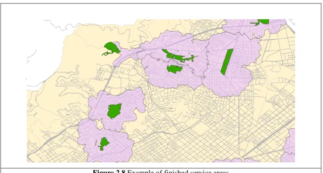
attribute, obtaining thus one composite service area for each one of the green spaces. Figure 2.8 illustrates an example of the resulting service areas.
Figure 2.8 Example of finished service areas
The process mentioned above is repeated for every green space category, in each case changing the impediment as defined in table 2.3. Once the service areas have been generated and merged based on the green space they emanate from (based on the Green ID attribute), we have as a final output of the network analysis a series of polygon shapefiles – one for each category – displaying area that is covered by each green space in each category. Local geometries, such as area, can be calculated for each service area as well as for each green space category as a whole. This information is useful to determine, for example, the total percentage of area in the municipality which is served – and thus considered to be accessible – by each green space category, as well as knowing the percentage of area of each neighbourhood which is covered by a service area in each category. The results conveying this information are presented in the results section coming ahead.
2.6 Spatial analysis
The following section is concerned with finding possible relationships between the distributions of clusters of accessible neighbourhoods and socio-economic characteristics of the residents. This is achieved following two distinct methodologies. First, we look for local indicators of spatial autocorrelation (LISA) as described by Anselin (1995) and following the works of Talen (1997) and Xiao et al. (2017). This is followed by the
19
application of the Mann-Whitney U test, which is useful for determining if the areas classified as “high access” and “low access” follow in any way the distribution of the socio-economic variables being studied. The combined results of these two methodologies will help us determine whether or not accessibility favours groups with particular socioeconomic characteristics over others (Talen, 1997).
The LISA analysis is performed by conducting a Local Moran's I statistic, which identifies spatial clusters of features with high and low values (Anselin, 1995; “How Cluster Analysis works”, 2016). The test can be used to determine the existence of statistically significant spatial clusters of single and/or bivariate variables (Talen, 1997; Xiao et al. 2017). The formula for the Local Moran’s I statistic is defined as follows:
𝐼𝑖 = ( 𝑧𝑖
∑ 𝑧𝑖 𝑖2) ∑ 𝑊𝑗 𝑖𝑗𝑍𝑗 (1)
Following the formula, zi and zj are expressed in deviations from the mean, while the summation over j only takes into consideration neighbouring values by using the spatial weights value Wij (Talen, 1997). A detailed explanation of the formula and the mathematics behind it is presented by Anselin (1995). The free and open source software GeoDa (version 1.6.7) was used to conduct this test. GeoDa is a tool specifically designed for conducting several forms of exploratory spatial data analysis, as well as spatial data regression and some others (“About GeoDa”, 2016). GeoDa provides an ideal environment for the production and processing of this type of data.
In the particular case of this work, the objective is to find spatial correlations between two variables at a given time; accessibility to green spaces by category on one side and a socio-economic variable (for example, income) on the other; due to this the bivariate Local Moran’s I test has been deemed as the most appropriate option. The results convey information about where both variables are clustered in the city, which aids in the discernment of possible spatial correlations. These results are displayed in the results section available below.
In addition to the results provided by the implementation of the bivariate Local Moran’s I, the Mann-Whitney U statistical test (also referred to as the Wilcoxon test) is applied to analyse the direct relationship between the distribution of park-accessible neighbourhoods and the spatial distribution of the selected socio-economic variables, following Talen (1997), Nicholls (2001) and Xiao et al. (2017). While the previous step
20
was aimed at finding correlations between the two, with the Mann-Whitney U test the objective is to assess whether or not a direct relationship exists between the areas that we have previously determined as “high access” and “low access” – based on the network service area analysis – and the distribution of the socio-economic variables in space. The Mann-Whitney U test is a non-parametric statistical test used to analyse if two independent groups of data could come from the same population, meaning that the two independent groups are homogenous and have the same distribution or, alternatively, whether or not observations in one sample tend to be larger than observations in the other (Shier, 2004). Being non-parametric, the Mann-Whitney U test does not require any assumptions about the distribution of the two groups of data, thus not requiring for them to follow a normal distribution. The test does however require the two samples to be mutually independent, meaning that a member of one cannot be present in the other. The formula is described as follows:
𝑈 = 𝑛1𝑛2+ 𝑛2(𝑛2+1)
2 − ∑ 𝑅𝑖 𝑛2
𝑖= 𝑛2+1 (2)
In this formula, n1 and n2 refer to the sample size of each group, and Ri is the rank of the sample. Referring to the application of statistical test in this research, the objective is to compare if there are statistically significant differences in the socio-economic variables in the areas deemed as “high access” and those that are “low access” for each green space category.
21
3. Results and discussion
This results section is divided into four parts. First, we analyse the results of the network-based service area analysis for each of the green space categories as well as the general distribution of green spaces and their respective areas of accessibility across the city. Then we proceed with a general overview of the spatial distribution of the socio-economic variables considered for this research in order to get insight in their distribution in respect to the already determined green area accessibility. Following that we examine the spatial clustering of the socio-economic variables and the park access. Finally, we analyse the equity in said distributions.
3.1 Accessibility and distribution of green spaces
Accessibility was determined for each green space category using the criteria established in table 2.3. The accessibility has been determined using the network-based service area approach as defined in the methodology section. Figures 3.1 through 3.5 display the maps conveying this information for each one of the green space categories. Each figure represents the accessibility map, based on the service areas with the distance impediment criteria for the park category and a choropleth map displaying the total area of each neighbourhood unit which is covered by a service area. The coverage has been classified into quartiles, with the lower quartile (light green) representing low access and the upper quartile (dark green) representing high access. For instance, a high access neighbourhood in the residential parks category would have access to a residential green space (minimum area of 0.1 ha) in less than 150 m from most points within the neighbourhood.
Figures 3.1a and 3.1b represent the accessibility for residential parks (0.1 ha minimum area and 150 m. maximum distance), which is the smallest green space type analysed in this research. In the case of our study area, these type of parks corresponded usually with small gardened areas usually in between mid-to-high density buildings. As these figures show, parks of this category are scattered across the entire urban area, and seem to enjoy from medium to high accessibility in most areas, especially in the eastern district of Sant Martí and in central areas of the city, between Les Corts and the Eixample (refer to figure 2.2 for reference about the districts). At first glance, there seems to be three big areas with a very low density of residential parks, on one hand we have the southern end of the municipality, which corresponds with southern Sants-Montjuïc. This area is occupied in part by the large Montjuïc Park – which belongs to the city park category – and by mostly non-residential port facilities. The north-western end of the municipality is also an area
22
with a very low density (figure 3.1a) and accessibility (figure 3.1b) to these parks. This is due to the fact that this area is home to the Natural Park of the Serra de Collserola, a large forested and mountainous area which is largely non-urbanised.
Figures 3.2a and 3.2b display the same information but for neighbourhood parks (1 ha minimum area and 400 m. maximum distance), the second smallest park category studied. The distribution looks very similar to that of the residential parks, although there seems to be larger empty areas across the central districts of Eixample and Gràcia. The western part of the Eixample district as well as the southern end of Gràcia, both in central Barcelona, are home to older neighbourhoods. These are very centric and with an apparent better distribution and accessibility to this type of parks.
In what refers to quarter parks (5 ha minimum area and 800 m. maximum distance), figures 3.3a and 3.3b show a more heterogeneous distribution in comparison to the first two park categories, with most quarter parks distributed in two corridors along the coastline and the transitional area between the city and forested area of the Serra de Collserola, which can be seen clearly in figure 4.3a. This leaves large areas of the Sant Andreu and northern Sant Martí districts by the eastern end of the city with less coverage, as well as sizeable areas of the Eixample and Gràcia districts. The southern neighbourhoods of the Sarriá Sant Gervasi district seem to also suffer from low accessibility, along with those in the Ciutat Vella district. These districts seem to form gaps of low accessibility within the distinct corridors formed by the successive parks. Figures 3.4a and 3.4b show an image clearly dominated by the only two parks of this category, the district parks (30 ha minimum area and 1600 m. maximum distance). The famous Park Güell and the neighbouring Guinardó Park produce a single cluster of high accessibility neighbourhoods which extends for 1.5 kilometres across the city, but still fails to offer coverage for most of the city districts. A clear deficit in this park category is thus evident, especially in the southern and western sections of the urban area.
23
24
25
26
27
28
Finally, figures 3.5a and 3.5b display the situation for city parks (larger than 60 hectares, with a maximum distance of 3.2 kilometres), which present a similar scenario, with a single park for the whole category. The Montjuïc Park is the largest urban green area in the city of Barcelona, located at the south-central part of the city and probably best known for being the home of the Olympic city. The service area is large enough to cover most of the southern districts, although due to the nature of the park (located on an elevated terrain overlooking the city), some areas at its back have a lower accessibility. Based on the reach of the service areas, it would seem the district parks (figures 3.4a and 3.4b) and the city park complement each other, each one providing availability to relatively large green spaces both in the northern and southern parts of the city, although it is important to remark that large areas like the Sant Marti, Sant Andreu and Nous Barris districts in the east, as well as the Les Corts in the west, are still unserved by either category. 3.2 Socio-economic characteristics
This section is focused on displaying the socio-economic variables introduced in table 2.1 from a spatial perspective. The variables used in this research are the following: i) income; ii) population density; iii) migrant population; iv) population younger than 15; v) population older than 60; and vi) buildings built before 1960. Figures 3.6 and 3.7 display the mapped spatial distribution of these socio-economic variables in the city of Barcelona. The aim behind displaying this information is to have a visual representation of the distribution of these variables in comparison with the distribution of park accessibility presented in the previous section (figures 3.1 through 3.5). The combined information is then analysed using the LISA maps in the following section. Figure 2.2 serves as a reference for the districts.
The spatial distribution of income is illustrated in the figure 3.6, map a, shown in standards deviations below and above the city average. It offers a pretty clear image, being notable that the higher than average income neighbourhoods appear to be clustered in the westernmost districts, particularly Les-Corts and Sarrià-Saint Gervasi, whereas the northern, eastern and southern areas of the city seem to concentrate lower than average income neighbourhoods. This distribution will be especially relevant when analysing how income influences accessibility. In what refers to density (figure 3.6 map b), Barcelona displays the characteristics of a high density city as it is usual in the country; Spanish cities tend to be very compact, leading to higher densities. The highest seem to be concentrated along a corridor in the central Eixample district.
29
30
31
Information about the spatial distribution of the migrant population is depicted in the figure 3.6 map c. This population seems to be clustered particularly around older neighbourhoods of the city, corresponding with the Ciutat Vella district and the areas by the port. In general the proportion of migrants appears to be higher in the half of the city closer to coast, which corresponds with older neighbourhoods as shown by map f in figure 3.7, which depicts the percentage of buildings built before 1960, and which are mostly concentrated around the old city as expected. Maps d and e from figure 3.7 depict the percentage of people younger than 15 and older than 60 respectively, and show a clear differentiation and apparent preference for newer, less dense neighbourhoods.
3.3 Spatial autocorrelation
The following part of this research focuses on finding spatial correlation or association between green space accessibility and the socio-economic characteristics. As it has been explained in the methodology section, the spatial correlation has been determined by conducting a bivariate Local Moran’s I test as proposed by Anselin (1995), the information then being displayed on LISA maps following the work of Xiao (2017). When conducting the test, the simultaneous presence of two variables is analysed; accessibility to each green area category on one hand (as determined by the network-based service areas and displayed on figures 3.1 to 3.5) and the socio-economic variables (figures 3.6 and 3.7 and table 2.1).
In each map presented below the neighbourhoods shown in dark red (High-High) represent high accessibility and a high presence of the socio-economic variable (income, for example), whereas those shown in light red (High-Low) represent high accessibility but a low presence of the socio-economic variable. In addition, areas shown in dark blue (Low-Low) represent a low accessibility and a low presence of the socio-economic variable, while light blue (Low-High) represent a low accessibility but a high presence of the socio-economic variable. Only neighbourhoods that are statistically significant are coloured. These clusters are determined by assessing whether or not each individual neighbourhood has high or low values and is also surrounded by other neighbourhoods with the same high or low values.
Figure 3.8 displays every LISA map for each socio-economic variable (columns) and each one of the green space categories (rows), numbered for an easier identification. The first column (maps 1a through 1e) display the distribution of high-low LISA values for income. Using map a) from figure 3.7 as a reference, it is evident that in the city of
32
Barcelona the distribution of income forms two relevant clusters, with high income neighbourhoods located in the north-western section of the city, particularly in western Barcelona (Sarrià-Saint Gervasi and Les Corts districts as depicted in figure 2.2), whereas low income neighbourhoods seem to be clustered in the opposite end of the city (mainly in the Nous Barris district). The high income districts seem to benefit from higher access in residential (map 1a) and neighbourhood parks (map 1b), although accessibility seems to have a slightly bigger correlation with low income neighbourhoods for quarter parks (map 1c).
In what refers to the distribution of high-low values for the population density variable, these are displayed on the second column (maps 2a through 2e). Figure 3.6 displays the population density of the city by neighbourhoods and can be used as a reference. The higher densities seem to be located in the central areas of the city, particularly in the Eixample and Sant Martí districts, which are in fact areas with a high density of buildings; the Eixample in particular is the central district of the city. When analysed alongside park accessibility, there seems to be a constant correlation between lower densities (particularly the Sarrià-Saint Gervasi district at the northwest) and lower accessibility values in all green space categories, which is to be expected. The denser areas in the Sant Martí and Eixample districts seem to have overall a high accessibility to residential and neighbourhood parks, respectively, as well as district parks (the only two parks in this category are located alongside the densest area of the city), however these areas seem to correlate with low accessibility for quarter and city parks.
33
34
The following column (maps 3a through 3e) displays the high and low distribution of values for the migrant population variable, for each one of the green spaces. Figure 3.6 displays the overall distribution of the migrant population in the city, and works as reference for the analysis. Across the city, the migrant population seems to be clustered in the neighbourhoods of the Ciutat Vella district – the old city, in the central-south part of the city – and with less intensity in the areas that surround it, particularly the Eixample. The north-eastern corner of the city is another hot spot, specifically the neighbourhoods of Trinitat Vella and Vallbona. These areas seem to correlate in certain degree with low income districts, as well as older neighbourhoods. These areas seem to correlate with low values of accessibility to quarter parks and particularly to district parks. Access to residential parks seems higher in the western half of the Ciutat Vella. From maps 3b and 3e it can be inferred that migrant populations enjoy good access to neighbourhood-type parks, as well as city parks; the Montjuïc Park is the only one on this category and is located in close proximity to the Ciutat Vella.
The next column (maps 4a through 4e) display information about the proportion of people younger than 15, along with the accessibility to each one of the green space categories. This information is expanded with the figure 3.7 that shows the overall distribution of population younger than 15 in the city. Age is considered an important variable when assessing park accessibility; young children and teenagers are more likely to visit a green space in their very immediate vicinity (Van Herzele and Wiedemann, 2003), and for this reason residential and neighbourhood parks have a special relevance with this population. The proportion of residents younger than 15 (figure 3.7 map d) seems to be located mostly far from the centre and along less dense (figure 3.6 map b) neighbourhoods. Following maps 4a and 4b it would appear that the population younger than 15 living in higher income areas (figure 3.7 map a) have a slightly better correlation with good accessibility areas to residential and neighbourhood green spaces, particularly the latter, than their low-income counterparts. Spatial correlations for the rest green space categories appear less clear.
The second to last column (maps 5a to 5e) displays mapped high-low values for the percentage of population older than 60 years old variable. In the particular case of this population group, it is considered that older people benefit from closer and smaller green spaces due to a limited mobility, usual on people of older age. Thus, especial relevance is given to residential and neighbourhood green spaces, which are represented by maps
35
5a and 5b. The overall proportion of people older than 60 (figure 3.7) serves as reference. Higher proportions of older populations seem to be mostly concentrated in the northern half of the city, particularly in the Horta-Guinardó and Nou Barris districts. This seems to correlate with high access to quarter and district parks (maps 5c and 5d). It would seem like the aforementioned districts have an overall low accessibility to residential and neighbourhood parks however.
The last column (maps 6a to 6e) depict the mapped LISA values for the last socio-economic variable considered on this research; the proportion of buildings built before 1960. The main interest behind the study of this variable is to determine if older neighbourhoods, most of them built during times where different models of urbanism were common practice, correlate spatially with worse accessibility values to all park categories. Figure 3.7 serves as reference. These neighbourhoods seem to be clustered in the central and southern parts of the city, along the Ciutat Vella and Eixample districts, which could be expected. It is interesting to notice however that there seems to be a spatial correlation with moderate high access to residential and quarter parks, and high access for neighbourhood and city parks, which would indicate that older neighbourhoods have a better park accessibility than initially anticipated.
3.4 Equity
This last section compares the socio-economic characteristics (variable by variable) of the neighbourhoods considered as “high access” versus those deemed “low access” to determine whether or not there is a statistically significant difference between those two populations based on their socio-economic characteristics. In regard to what is considered “high access” and “low access” in the context of this test, the approach suggested by Talen (1997) was considered the most appropriate. Considering the results obtained from the service area analysis (figures 4.1 to 4.5), those neighbourhoods located in the lower quartile of the distribution were considered to be “low access”, whereas those in the upper quartile are deemed to be “high access”. In order to produce this test, the Mann-Whitney U test has been employed using R, as it has been introduced on the methodology section. Table 3.1 displays the medians for the high access and low access neighbourhoods for each one of the variables as well as for each one of the green space categories. The Mann-Whitney U test has been implemented to compare the high access population of each variable with the low access counterpart. This is a non-parametric test as it does not assume normality. The null hypothesis (p-value > 0.05) is that there is not any statistical
36
difference between the two populations (that could be identical), whereas the alternative hypothesis (p-value < 0.05) establishes that there are indeed statistical differences between the populations (Talen, 1995). In the context of this research, a rejection of the null hypothesis would mean that indications exist to make the affirmation that the socio-economic variables have some effect on the distribution of high and low accessibility to the green areas. Otherwise, we would conclude that no such effect exists.
Park type Variable High access (median)
Low access
(median) W p-value* Equity?
Residential Income 85.8 77.4 119 0.07472 Yes
Density 34791.4 11577.9921 89 0.006829 No
Migrants 13.6 12.2 135.5 0.1937 Yes
Younger than 15 12.6 12.7 190.5 0.7811 Yes
Older than 60 22.6 21.9 176.5 0.9186 Yes
Built before 1960 28.3 31.2 171 0.7927 Yes
Neighbourhood Income 76.8 72.7 151.5 0.4054 Yes
Density 29252.0817 19202.6205 137 0.212 Yes
Migrants 12.9 15.1 189 0.8153 Yes
Younger than 15 13 14.1 233 0.2199 Yes
Older than 60 22.3 20.1 148 0.3499 Yes
Built before 1960 25.7 26.8 191 0.7729 Yes
Quarter Income 76.8 79.6 171 0.7951 Yes
Density 29252.0817 25839.6708 190 0.7951 Yes
Migrants 14 13.2 155.5 0.4741 Yes
Younger than 15 13.8 13.1 174.5 0.8723 Yes
Older than 60 21.2 20.6 166 0.6826 Yes
Built before 1960 28.3 30.4 199.5 0.5891 Yes
District Income 83.3 77.2 348 0.4316 Yes
Density 34595.1836 20741.8405 234 0.009549 No
Migrants 13.2 16.7 478 0.2214 Yes
Younger than 15 13.1 13.35 456.4 0.3744 Yes
Older than 60 22.9 19.85 202.5 0.002263 No
Built before 1960 30.8 28.05 340.5 0.3664 Yes
City Income 97.8 75.75 233 0.001968 No
Density 32856.2615 23775.7842 351 0.1471 Yes
Migrants 18.2 12.9 238 0.002475 No
Younger than 15 11.9 13.7 729.5 1.45E-04 No
Older than 60 21.3 22.5 580.5 0.08445 Yes
Built before 1960 46.1 26.8 255 0.005286 No
* Null hypothesis: p-value > 0.05. Alternative hypothesis: p-value < 0.05 Table 3.1 Mann-Whitney U analysis of park access equity
37
Analysing the results yielded by table 3.1 we can see that, for the most part, it does not seem like there are significant differences in the overall access to green spaces for most socio-economic characteristics; the distribution of high access and low access areas seems to be equitable. District green spaces and city green spaces (or city parks) seem to be the only two green space categories with significant inequities in distribution. Comparing these results with figures 3.4 and 3.5 we can see that these inequities are most likely causes by the fact that there is a very limited number of parks on this category for the whole municipality: two parks for the district category (the two adjacent to each other) and located in the northern half of the city, and one single park for the city park category, located in the south. It is likely that if these two parks were considered together they would function as complementary, however they have very stark differences in size and characteristics (39 ha in both cases for the district parks against close to 326 ha for the city park) for this to be a realistic scenario.
In the particular case of residential parks, there seems to be inequity by the population density variable, although the spatial correlation does not seem very clear. Interestingly, significant inequities by income and proportion of migrant population do not seem to exist, despite these two being common due to the nature of said socio-economic variables. City parks seem to show inequities in both, this can be explained however by the location of the single city park (Montjuïc Park) in the southern region of the city, very close to the old town, where there are bigger proportions of migrant populations and older buildings, as shown by the inequities in both categories and figures 3.6 and 3.7; in addition higher income neighbourhoods seem to be clustered in the north-western section of the city, relatively far from the Montjuïc Park, which explains the results.
It is a common argument that low income and migrant populations are often marginalised from good accessibility to urban services, including in many cases green areas. This does not seem to be the case in Barcelona, as the results indicate that for all but one green space category there seems to be equity in access. The migrant population also seem to be in a positive situation as significant inequities were not found for their population; in fact migrant populations seem to be positively affected by a circumstantial inequity in the city park category.