A Work Project, presented as part of the requirements for the Award of a Master Degree in Economics from the NOVA – School of Business and Economics
FISCAL DYNAMICS AND ELECTORAL BEHAVIOR IN THE EUROZONE
INÊS GONÇALVES RAPOSO 743
A Project carried out on the Master in Economics Program, under the supervision of Prof. José Tavares
January 2016
08
Fall
Fiscal Dynamics and Electoral Behavior in the Eurozone
Abstract: The Stability Growth Pact and the 3% rule did not prevent countries from running large deficits. Countries in the EMU administrate fiscal policies differently, despite the existence of a common quantitative goal. The main focus of this work project is to study differences in the fiscal dynamics of eight EMU countries and assess the role of political variables in shaping those dynamics. We find that elections negatively affect government revenue in Austria, Belgium, Portugal, Spain and Germany. Expenditure, on the other hand, responds positively to incoming elections in Portugal, Italy, France and Netherlands, and negatively in the case of Germany.
Keywords: Fiscal dynamics, SVAR, EMU, elections
The author would like to thank Professor José Tavares for his help and enthusiasm. Acknowledgments are also due to Professors Paulo Rodrigues, Luís Catela Nunes and Francesco Franco, for their kind inputs. A final word of gratitude goes to my colleague and friend Jaime Marques Pereira, for his suggestions and interest, and to my parents, for their endless patience and support.
1. Introduction
Fiscal discipline is a challenge for most countries. Beyond its macroeconomic effects, deficit reduction policies also have political consequences. The study of fiscal dynamics has renewed importance for Eurozone countries - with no discretionary power over monetary policy, fiscal policy is the main instrument for cyclical stabilization, as Buti et al. (2003) point out.
In this work project, we assess fiscal dynamics in eight EMU countries making use of quarterly data from 1999 to 2015. A pertinent research issue is whether policy differences are attenuated after political variables are taken into account in the model, and to describe how political variables themselves affect different countries. A Structural Vector Autoregressive model following the Blanchard-Perotti identification scheme is estimated for each of the countries in order to retrieve the responses of government revenue and spending to unanticipated fiscal shocks. The impact of political variables on government revenue and expenditure is also quantified. Although no evidence of partisan effects is found for the countries in sample, a statistically significant electoral effect is present. Incorporating the timing of elections into the model approximates countries that had similar initial dynamics. This work project is organized as follows – Section two provides a brief literature review, summarizing the current state of the art. Data properties are described in section three. The methodology is explained in section four. Section five presents the main empirical results and section six concludes with some final remarks and suggestions for further research.
2. Related Literature
The Maastricht Eligibility Criteria and, later, the Stability Growth Pact were seen as an incentive to achieve low levels of public deficit and have budgetary positions converge across countries in the EMU. After accession, however, some convergence fatigue might have set in1 and compromised fiscal sustainability. In reality, after the third stage of the EMU, some countries faced large and growing deficits. Southern European countries, in particular, were accused of engaging in irresponsible behavior through excessive lending, allegedly made possible by the common currency’s credibility. However, although these countries face ongoing Excessive Deficit Procedures, almost every country of the EMU has breached the 3% rule at some point. What is the dynamic response of fiscal variables, and how does it differ across EMU countries? Are differences attenuated when political factors are accounted for? Four main different theoretical hypotheses attempt to describe the intertemporal relation between public revenues and expenditures - the spend-tax hypothesis, the tax-spend hypothesis, the fiscal synchronization hypothesis and the institutional separation hypothesis. The spend-tax hypothesis argues that changes in expenditure lead to changes in taxes. Conversely, under the tax-spend hypothesis, changes in tax revenues motivate changes in expenditures. If positive changes in taxation lead to positive changes in government spending and vice-versa, the ‘starve the beast’ hypothesis is verified. If, on the other hand, there is an inverse relation between taxes and spending, the fiscal illusion hypothesis is verified. The third view, the fiscal synchronization hypothesis, suggests that policymakers decide on government spending and revenue simultaneously. Finally, under the institutional separation hypothesis, decisions concerning spending and revenue are independent from each other and there is an absence of any causal relation.
Typically, empirical studies on this matter focus on a single country set up and rely on co-integration procedures, error correction models and Granger causality tests. Payne (2003) provides an extensive survey of the empirical literature on the subject at national and subnational levels, with the majority of studies located on the United States. Romer and Romer (2009) use the narrative approach and find a positive effect of tax cuts on spending, but no evidence of the ‘starve the beast hypothesis’ for the United States is found. Kollias and Paleologou (2006) use a VECM framework for each of the EU15 countries during the 1960-2002 period and find evidence supporting the fiscal synchronization hypothesis for Denmark, Greece, Ireland, Netherlands, Portugal and Sweden. Austria, Belgium and Germany are in conformity with the institutional separation hypothesis. Italy and Spain verify the tax-and-spend hypothesis. The authors find evidence that lower taxes lead to higher expenditure for Finland and France.
Recently, there has been a growing body of literature analyzing the effects of fiscal policy shocks with the recourse to the Vector Autoregressive models. The use of identification schemes and a Structural Vector Autoregressive framework enables the separation of true policy shocks from cyclical reactions. Blanchard and Perotti (2002) use extra-model information on elasticities of fiscal variables to output and conclude that unanticipated tax increases affect output negatively. Their identification methodology has, to some extent, become the benchmark for this type of studies. Other existing identification schemes include the recursive identification (Sims, 1980), the sign-restrictions approach (Uhlig, 2005) and the event-study approach (Ramey and Shapiro, 1998). Caldara and Kamps (2008) provide a brief explanation of these identification methods and show how results on fiscal multipliers diverge depending on the chosen identification method. Afonso and Claeys (2008), through the estimation of a Vector Autoregressive Model and the construction of an indicator of structural balance for France, Germany, Portugal and Spain, conclude that there is a procyclical bias in
fiscal policies – governments cut taxes during booms, but these cuts are not accompanied by cuts in spending, leading to deficits when economic conditions worsen.
Another strand of the literature concerns the political economy of fiscal policy. Political factors and the institutional environment will ultimately influence how fiscal policy is conducted. Harden et. al (1994) emphasize the role of institutions in the budget process as determinant for fiscal performance. The timing, duration, composition and degree of success of a fiscal adjustment may also be influenced by economic and political-institutional factors, some of them being political stability, the existence of organized interest groups or the degree of transparency (Mierau, 2007). Mulas-Granados (2003) examines the political and economic determinants behind EU-15 countries following different fiscal strategies in the period from 1990 to 2001. He finds that economic conditions, fragmented decision-making, government size, ideology and closeness to elections all affect budget composition in adjustment and non-adjustment years. In Eurozone countries, fiscal policy is the only instrument to influence voters’ perceptions prior to elections. In this sense, it is reasonable to expect some degree of political manipulation to occur. Indeed, Buti and van den Noord (2003), Mink and de Haan (2006) and Efthyvoulou (2012) find evidence of electoral fiscal policy manipulation in the Eurozone during the early years and thereafter. These studies make use either of a qualitative approach or univariate econometric analysis and do not take into account the contemporaneous and lagged relations between variables. Testing political economy hypotheses using time series methodologies is not common heretofore.
In sum, although there is considerable literature that assesses the spending and taxation nexus and the determinants of fiscal policy in European Union countries, testing for the relevance of politico-institutional factors as determinants of fiscal dynamics has been an overlooked topic. This work project combines the aforementioned two strands of literature, making use of the powerful time series methodology to shed light on the role of political factors in fiscal policy.
3. Data
Quarterly data was extracted from Eurostat from the first quarter of 1999 to the first quarter of 2015 for the following countries – Austria, Belgium, Germany, France, Netherlands, Spain, Portugal and Italy.2 Estimates of fiscal elasticities are from the OECD.3 Political variables were obtained from the Supplement to the Comparative Political Data Set until 2013 and updated to 2015 using complementary information from the Adam Carr’s Election Archive. More information on data description and sources can be found on Appendix 1. The use of quarterly data allows for more degrees of freedom in estimation and is essential for the identification assumption that considers fiscal variables do not react to output shocks within the quarter. The use of high frequency data is thus recommended since it allows for a more accurate identification of the effects of fiscal shocks.
The first step of the analysis consists in examining the time series properties of the data. In this sense, Augmented Dickey Fuller and Phillips-Perron tests were performed to test for non-stationarity. The ADF test was performed using a constant and no trend and the choice of the number of lags was made according to the Schwarz Information Criterion (SIC). For all countries, the null of unit root cannot be rejected at 5% significance level. When expressed in first-differences, all series are stationary. Often in the literature, VARs are estimated in levels with the underlying assumption of a cointegration relationship between variables. If that is not the case, the model will be misspecified and estimates of the impulse response functions will be biased. In this sense, the Johansen’s maximum likelihood cointegration rank test is run. For every country the results do not reject the null of no cointegration amongst the variables in levels. The model is then specified in first-differences.
2 Total government expenditure, total government revenue and GDP were originally in nominal terms and
non-seasonally adjusted. The series were non-seasonally adjusted using X-13, deflated using the GDP deflator and log-transformed.
3 See OECD “Estimates for EU Budget Surveillance” (2014). More recently, ECFIN has published “Tax
Revenue Elasticities Corrected for Policy Estimates in the EU” (November, 2015). These are revenue-to-base, and not revenue-to-output elasticities. For this reason, and to use the same source for revenue and expenditure elasticities, we opt for the 2014 OECD Estimates.
4. Methodology
The baseline empirical model consists on a three-variable Vector Autoregressive Model of revenue, expenditure and GDP, all expressed in first differences and log-transformed. The model in reduced form can be presented as:
𝑦!= 𝐴 𝐿 𝑦!!!+ 𝑢! (1)
where A(L) is a lag polynomial of order p, yt=(Δtt,Δgt,Δxt), E[ut]=0 and E[utu’s]=0 for t ≠ s. A
constant and intervention dummies to control for the beginning of the economic and financial crisis were included. The number of lags p used in each model was chosen using the Schwarz Information Criterion, with a maximum of four lags imposed. Tests for autocorrelation, normality of the residuals, heteroskedasticity and parameter stability were performed in order to assure model adequacy, presented on Appendix 3.
If the VAR is stable, it is invertible and has a Wold Moving Average representation that expresses the vector of endogenous variables as a function of past shocks in the system.
!!!! ! !!!!,
!!!!!!!
(2)
The model can be presented as a function only of unexpected structural innovations et by
imposing some restrictions. Structural disturbances, or innovations, are assumed to be uncorrelated and their covariance matrix diagonal. In order to identify the model, at least nine restrictions are needed. The assumption of orthogonality of structural shocks imposes six restrictions. We impose the remaining three restrictions following the Blanchard and Perotti (2002) approach. That is, information from external institutions is used so that discretionary policy changes are treated as unexpected policy shocks and are separated from automatic stabilizers effects. This way, one is able to extract the ‘pure’ policy effect. The underlying logic is that unexpected movements in fiscal variables happen either because of automatic stabilizers or discretionary policy changes. In this identification scheme, discretionary policy changes correspond to the structural shocks. The effects of automatic stabilizers are accounted
for through the use of elasticities. Blanchard and Perotti (2002) express the relationship between the reduced form and structural form shocks as follows:
𝑡!= 𝑎!𝑥!+ 𝑎!𝑒!!+ 𝑒! ! 𝑔! = 𝑏!𝑥!+ 𝑏!𝑒!!+ 𝑒!! 𝑥! = 𝑐!𝑡!+ 𝑐!𝑔!+ 𝑒!!
(3)
Where (tt gt xt) are the reduced form shocks and (ett egt ext) are the structural shocks for
government revenue, expenditure and output, respectively. Expressing this relation in matrix form yields the equivalent notation Aut=Bet, with
A = 1 0 −𝑎! 0 1 −𝑏! 𝑐! 𝑐! 1 and B = 1 𝑎! 0 𝑏! 1 0 0 0 1 (4)
Unemployment-related spending is cyclically sensitive and is included in our measure of government spending. Thus, contrary to Blanchard and Perotti, b1 is not set to zero, as their
assumption that spending does not react to changes in output within the quarter does not apply in this case. Values for a1 and b1 are computed using the latest OECD Surveillance Estimates,
with appropriate adjustment.4 The final restriction consists in the assumption that tax decisions are made prior to spending decisions (a2=0) or the inverse (b2=0). We estimate both
models and found differences in resulting IRFs negligible. For the sake of space, only the model where we assume tax decisions are taken first is presented. The used elasticity estimates are presented in Appendix 1. With these restrictions, the model is exactly identified and one is able to retrieve the impulse response functions and infer on the differences in fiscal dynamics across countries.
It is reasonable to think the ideological stance of the party in government or the run up to elections both can influence spending or taxation levels. One would expect left cabinets to run
4 The revenue elasticity measure uses the aggregated tax elasticity measure provided in the report multiplied by
the share of tax revenue on total government revenue. The expenditure elasticity measure is attained multiplying the share of unemployment related spending in expenditure by the output elasticity of unemployment related spending.
higher spending and taxes in general, as well as higher spending and lower taxes before elections. If these factors matter, the baseline model, which ignores them, suffers from omitted variable bias. Thus, political variables are added exogenously into the model and their impact is analyzed in three ways – first, we check if the sign and statistical significance of the coefficients in the reduced form VAR are appropriate; second, the cumulative dynamic multipliers are computed from the reduced form VAR to see how a change in the political variable impacts the fiscal variables along time.5; third, the structural model with the new
exogenous variables is re-estimated and resulting IRFs are compared with the baseline case. Accumulated IRFs present the responses of the variables in levels and are originally computed as the responses to one standard deviation shocks in revenue and spending. In order to express the shocks in percentages, allowing for a more intuitive reading of the results, the accumulated impulse response functions are divided by the standard deviation of the structural shock.6 We investigate the effects of a positive spending shock and of a negative revenue shock. Focusing on a negative revenue shock allows for a more interesting interpretation of dynamics, as both responses – spending increase or tax decrease – can be seen as a reaction to a shift away from budgetary equilibria. This is possible since IRFs are symmetric in sign. The response to a negative shock is simply the symmetric of the response to a positive shock.
The expanded VAR can be expressed as
𝑦! = 𝐴 𝐿 𝑦!!!+ 𝛿!𝑒𝑙𝑒𝑐!+ 𝛿!𝑙𝑒𝑓𝑡!+ 𝑢! (5)
The inclusion of exogenous variables has no impact on the identification process.
5 We compute the cumulative dynamic multipliers to obtain the responses of the variables in levels instead of
first-differences. As the dependent variable is specified in logarithms and the innovation is in levels, multiplying the coefficient by 100 yields an approximation of the response in percentage points.
6 This is, responses to a shock in spending were divided by the standard deviation of the spending shock. The
same applies for responses to shocks in revenue. Information on estimated standard deviations and structural factorizations can be found on the Technical Appendix.
5. Empirical Results
The results for the baseline and expanded models are presented below. The inclusion of the partisan dummy was not statistically significant for any country. We tried including different political indicators, including whether cabinet posts or parliamentarians supporting the government were majoritarian left-wing. None was significant. Consequently, the partisanship indicator was dropped from the analysis.
The electoral dummy was defined having in mind anticipation effects – it is unlikely that changes in spending and taxation in the hope of reaping electoral benefits occur in the same quarter as the election date, as fiscal policy decisions take some time to plan, implement and come into fruition. So we set the dummy to 1 in the four quarters prior to the election quarter. Panel 1 of Figure 1 synthesizes the countries’ dynamics twenty quarters after a 1% positive shock in government spending or a -1% shock in government revenue. We can see that the signs of the government spending responses to an unanticipated contraction in revenue are different. Southern European countries - Italy, Portugal, Spain -, along with France, increase spending when faced with a negative shock in revenue. This is in line with the ‘fiscal illusion’ hypothesis – taxpayers do not fully perceive the cost of government and demand greater spending. The remaining countries – Belgium, Austria, Netherlands and Germany – adjust spending negatively, moving toward deficit containment. This is line with the ‘starve the beast’ hypothesis. On the other hand, when government spending expands unexpectedly, Southern Europe countries, along with Germany and Austria increase revenue, whereas France, Belgium and Netherlands have the opposite reaction. It is noticeable that Southern European countries have distinct dynamics from other countries in sample, being located in the same quadrant. It is also important to note that, as the co-integration hypothesis is rejected, it is not possible to infer about the existence and direction of causality between
revenue and spending. We focus on adjustments dynamics – this is, given a discretionary change in one side of the budget, we analyze how the other side responds.
Panel 2 of Figure 1 presents the dynamics when the electoral variable is taken into account in the model specification. The inclusion of the electoral variable brings responses of countries with initial similar dynamics closer, as can be seen for Portugal and Spain. There are no changes in the signs of the responses, and very few changes in magnitudes, except in the case of Germany and Spain. A better depiction of these movements can be seen in Figure 2. For Germany, it is possible to see that the inclusion of the electoral dummy makes revenue more responsive to a positive shock in spending. Spending, on the other hand, is less responsive to a negative shock in revenue when elections are taken into account. This is, a positive shock in spending causes a larger expansion in revenue. A negative shock in revenue causes spending to contract less than it normally would.
As for Spain, the inclusion of the electoral dummy makes revenue less expansive to positive shocks in spending, and spending more expansive given a negative shock in revenue. These movements are also seen for Portugal and Italy. It is interesting to find the inclusion of the electoral dummy causes a clear shift away from budgetary equilibrium in the case of Southern European countries, but partially enhances consolidation for Germany. A possible explanation for this that could be explored in the future would be that voters reward the incumbent differently in each country.
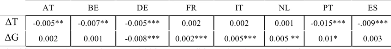
In order to quantify the effect of the inclusion of the electoral dummy, Table 1 presents the estimated coefficients on the reduced form model. We can observe upcoming elections have a negative impact on revenue change in Austria, Belgium, Germany, Portugal and Spain. An increase in spending is found in the cases of Italy, Portugal, France and the Netherlands. A decrease in spending is found for Germany.
The percentage impact on total government revenue and total government expenditure is presented in Figures 3 and 4. Tables 2 and 3 provide complementary information to the understanding of the graphics. From there, it is possible to see that the immediate impact of an upcoming election on total government revenue is of -0,7% for Belgium, -1,5% for Portugal, -0,5% for Austria and of 0,5% for Germany, vanishing subsequently. The impact is of 0,57% for Spain, but it is not statistically significant. The electoral effect is only felt after one quarter and by the end of the first year, with a 0,97% reduction in revenue.
On the expenditure side, the immediate impact of upcoming elections is of -0,8% for Germany, 0,25% for France, 0,46% for Italy and 0,46% for Netherlands. This effect persists only for Netherlands and Italy, with the one-year impacts of 0,6% and 0,28%, respectively. By the end of first year, there is a 0,8% increase in spending for Portugal.
In sum, although the inclusion of the electoral dummy has a statistically significant impact on fiscal variables, this impact is short-lived and does not greatly influence fiscal dynamics in the long-run.
Table 1. Estimated VAR Coefficients for the Electoral Dummy
AT BE DE FR IT NL PT ES
ΔT -0.005** -0.007** -0.005*** 0.002 0.002 0.001 -0.015*** -.009*** ΔG 0.002 0.001 -0.008*** 0.002*** 0.005*** 0.005 ** 0.01* 0.003 Significance at *90%, **95% and ***99% confidence levels, respectively
-‐.4 -‐.2 .0 .2 .4 -‐.4 -‐.2 .0 .2 .4
% response in T to a 1% shock in G
% r es po ns e in G to a -‐1 % s ho ck in T DE ES PT FR IT BE AT NL Panel 1 -‐.4 -‐.2 .0 .2 .4 -‐.4 -‐.2 .0 .2 .4
% response in T to a 1% shock in G
% r es po ns e in G to a -‐1 % s ho ck in T FR BE NL IT ES PT DE AT Panel 2
Figure 1. Dynamic Responses of Government Spending and Revenue 20 quarters after the shock
-‐.4 -‐.2 .0 .2 .4 -‐.4 -‐.2 .0 .2 .4 Baseline Model Electoral-‐Dummy Model DE AT BE FR IT NL PT ES
% response in T to a 1% shock in G
% r es po ns e in G to a -‐1 % s ho ck in T Figure 2. Comparison of Budgetary Dynamics between Models.
Responses in percentage points, 20 quarters after the shock.
-‐1.00 -‐0.75 -‐0.50 -‐0.25 0.00 0.25 0.50 0.75 1.00 2 4 6 8 10 12 14 16 18 20 -‐1.2 -‐0.8 -‐0.4 0.0 0.4 0.8 1.2 2 4 6 8 10 12 14 16 18 20 -‐2.0 -‐1.5 -‐1.0 -‐0.5 0.0 0.5 1.0 1.5 2.0 2 4 6 8 10 12 14 16 18 20 Germany -‐2.4 -‐2.0 -‐1.6 -‐1.2 -‐0.8 -‐0.4 0.0 0.4 2 4 6 8 10 12 14 16 18 20 Spain -‐3.0 -‐2.5 -‐2.0 -‐1.5 -‐1.0 -‐0.5 0.0 0.5 1.0 2 4 6 8 10 12 14 16 18 20 Portugal Austria Belgium Figure 3. Cumulative Dynamic Multipliers. Total Government Revenue.
Responses in percentage points, presented with 95% confidence level interval bands.
Table 2. Cumulative Multipliers on Total Government Revenue
quarters BE DE ES AT PT
0 -0,702 ** -0,523*** -0,571 -0,497 ** -1,512***
1 -0,231 -0,396 -0,817 ** -0,177 -0,430
4 -0,263 -0,597 -0,971 ** -0,120 -0,885
-‐1.00 -‐0.75 -‐0.50 -‐0.25 0.00 0.25 0.50 0.75 1.00 2 4 6 8 10 12 14 16 18 20 France -‐1.00 -‐0.75 -‐0.50 -‐0.25 0.00 0.25 0.50 0.75 1.00 2 4 6 8 10 12 14 16 18 20 -‐1.5 -‐1.0 -‐0.5 0.0 0.5 1.0 1.5 2 4 6 8 10 12 14 16 18 20 Germany -‐2.0 -‐1.5 -‐1.0 -‐0.5 0.0 0.5 1.0 1.5 2.0 2 4 6 8 10 12 14 16 18 20 Netherlands -‐2.0 -‐1.5 -‐1.0 -‐0.5 0.0 0.5 1.0 1.5 2.0 2 4 6 8 10 12 14 16 18 20 Portugal Italy Figure 4. Cumulative Dynamic Multipliers, Total Government Spending.
Responses in percentage points, presented with 95% confidence level interval bands.
Table 3. Cumulative Multipliers on Total Government Spending
quarters DE FR IT NL PT
0 -0,836*** 0,247 *** 0,456 ** 0,459 ** 0,962
1 -0,702*** 0,104 0,316 ** 0,543 ** 0,563
4 -0,527 0,130 0,283 ** 0,597** 0,757 ***
6. Conclusion and Final Remarks
In this work project I have characterized the fiscal dynamics in EMU countries and tested whether existing differences are attenuated after considering political factors. As a result, two groups of countries are clearly identified. Countries that, when faced with a surprise negative shock in government revenue, cut spending, and countries that do the opposite and expand spending. The inclusion of an electoral dummy is statistically significant, yet it changes dynamics very little, either in terms of the sign or as far as the size of coefficient. It attenuates differences between countries that were already similar.
This work adds something to the existing literature, as the use of time series methodologies to assess political hypothesis is not exploited thus far. The use of updated information on elasticities is another advantage. Finally, studies on fiscal dynamics tend to focus on the pre-crisis period and do not take information after 2008 into account. If fiscal policy is determinant for stabilization purposes, it is of the utmost importance to assess its behavior precisely during periods of instability. The fact that Southern Europe countries’ reactions contrast with the others should also be highlighted, given the current political context.
There are several avenues for future research that can complement the results presented here. The first one encompasses the treatment of the crisis period, which may be adding noise to the model, despite the stability tests that were performed. Intervention dummies have been used as a way to control for the changes in this period, yet other methodologies can be used in conjunction with tests for structural breaks in the VAR. Another possibility would be to estimate the model with an alternative sample excluding the crisis period, albeit the small dimension of the resulting sample. Finally, a more detailed account of fiscal dynamics would be interesting to analyze which components of government revenue and expenditure are more sensitive to election dates and how do they adjust.
Appendix 1. Data Definitions and Sources
Definition Data Source
tt Quarterly total general government revenue,
million euros, in real terms, seasonally adjusted
Eurostat Quarterly non-financial accounts for general government (series code: gov_10q_ggnfa)
gt Quarterly total general government expenditure,
million euros, in real terms, seasonally adjusted
Eurostat Quarterly non-financial accounts for general government (series code: gov_10q_ggnfa)
yt Quarterly Gross domestic product, million euro,
in real terms, seasonally adjusted
Eurostat Quarterly national accounts: GDP and Main components (output, expenditure and income) (series code: namq_10_gdp )
def Quarterly GDP deflator, 2010 reference year, seasonally adjusted
Quarterly national accounts: Volume and Price indices – GDP Expenditure approach Series: B1_GE Measure DOBSA
𝛼 Output elasticity of government revenue OECD New Tax and Expenditure Elasticity Estimates for EU Budget Surveillance, Table 8 Column 1
𝛾 Output elasticity of government expenditure OECD New Tax and Expenditure Elasticity Estimates for EU Budget Surveillance, Table 9 Columns 1 and 2
Other
Parliament election dates
Government composition 1: Relative power position based on cabinet posts
Government composition 2: Relative power position based on parliamentary seat share
Supplement to the Comparative Political Data Set – Government Composition 1960-2013.
Adam Carr’s Election Archive, for election dates from 2013 to 2015
Elasticities used in Estimation
AT BE DE FR IT NL PT ES
𝑎! 1,02 1,03 0,99 1,02 1,07 1,08 0,96 1,02
Appendix 2. Unit Root and Cointegration Tests
Appendix 2.1 Unit Root Tests
Country Augmented Dickey Fuller Phillips-Perron
Levels Differences First Levels Differences First Austria Ln G -1.157 -5.899*** -1.444 -16.625*** Ln T -2.992 -4.161*** -0.008 -9.263 *** Ln Y -1.685 -6.612*** -2.262 -5.380*** Belgium Ln G -2.334 -6.246*** -0.556 -9.194 *** Ln T -3.028 -5.854*** -1.427 -13.092*** Ln Y -1.393 -3.987*** -2.160 -3.966*** France Ln G -1.584 -5.244*** -1.310 -10.267*** Ln T -0.929 -6.683*** -1.216 -12.504*** Ln Y -1.895 -4.520*** -2.759 -4.744*** Germany Ln G -0.688 -5.810*** -1.031 -9.820*** Ln T -0.873 -3.964** -0.581 -7.435*** Ln Y -0.983 -3.987*** -1.168 -3.966*** Italy Ln G -1.034 -6.003*** -2.331 -11.208*** Ln T -2.112 -6.426** -3.108** -21.722*** Ln Y -2.256 -3.358** -2.303 -3.909*** Netherlands Ln G -1.734 -6.873** -1.449 -8.291*** Ln T -0.813 -4.369*** -1.100 -10.095*** Ln Y -1.537 -3.642*** -2.415 -4.223*** Portugal Ln G -2.186 -6.006*** -2.408 -13.569*** Ln T -2.109 -6.943*** -2.042 -11.844*** Ln Y -1.657 -3.378*** -2.512 -8.845*** Spain Ln G -1.759 -7.109** -2.051 -8.355*** Ln T -2.447 -2.884** -1.974 -6.170*** Ln Y -1.762 -2.062** -4.103*** -9.403***
Rejection of null of nonstationarity at *** 99% and ** 95% confidence levels, respectively. Use of 61 observations for Belgium, France, Italy, Netherlands and Portugal; 49 observations for German and Spain; 53 observations for Austria.
The ADF test performed with constant, no trend and four lags. The 5% critical value is -3.50 (Fuller, 1976).
Appendix 2.2 Cointegration Tests
Trace Test Prob Max eigenvalue Prob
AT 31,191 0,127 19,701 0,111 BE 21,166 0,347 10,827 0,665 DE 26,457 0,116 16,251 0,211 ES 35,064 0,011 18,691 0,106 FR 25,804 0,135 18,397 0,116 IT 23,789 0,210 13,295 0,423 NL 26,800 0,107 17,193 0,163 PT 21,868 0,306 11,765 0,571
Null hypothesis: No-cointegration. MacKinnon-Haug-Michellis (1999) p-values. Estimation with 3 lagged diferences. 95% critical values are 35,19 and 22,3, respectively.
Appendix 3. Tests for Model Adequacy
Appendix 3.1. Tests for Model Adequacy – Baseline Model Normality of Residuals and Heteroskedasticity Tests
AT BE DE ES FR IT NL PT
(I) 0,790 0,507 0,289 0,805 0,381 0,193 0,309 0,977 (II) 0,704 0,702 0,412 0,448 0,966 0,192 0,599 0,956
(I) p-values for Joint Jarque-Bera Residual Normality test. Null hypothesis: Residuals are multivariate normal
(II) p-values for Joint White's Residual Heteroskedasticity test. Null hypothesis: No heteroskedasticity in residuals
VAR Residual Serial Correlation LM Test
Lags AT BE DE ES FR IT NL PT
1 0,237 0,416 0,457 0,500 0,666 0,966 0,683 0,275 2 0,099 0,192 0,096 0,627 0,398 0,097 0,187 0,529 3 0,516 0,312 0,107 0,230 0,181 0,146 0,072 0,199 4 0,406 0,735 0,958 0,998 0,273 0,486 0,487 0,491
Appendix 3.2. Tests for Model Adequacy – Expanded Model Normality of Residuals and Heteroskedasticity Tests
AT BE DE ES FR IT NL PT
(I) 0,726 0,574 0,539 0,691 0,950 0,152 0,402 0,964 (II) 0,631 0,836 0,424 0,586 0,978 0,09 0,492 0,961
(I) p-values for Joint Jarque-Bera Residual Normality test. Null hypothesis: Residuals are multivariate normal
(II) p-values for Joint White's Residual Heteroskedasticity test. Null hypothesis: No heteroskedasticity in residuals
VAR Residual Serial Correlation LM Test
Lags AT BE DE ES FR IT NL PT
1 0,130 0,437 0,129 0,645 0,382 0,934 0,914 0,274 2 0,102 0,216 0,143 0,667 0,401 0,234 0,202 0,525 3 0,964 0,371 0,052 0,081 0,231 0,083 0,155 0,178 4 0,372 0,691 0,668 0,965 0,346 0,375 0,811 0,298
References
Afonso, António, Claeys, Peter. (2008). “The dynamic behaviour of budget componentes and output,” Economic Modelling, Elsevier, vol.25(1), pages 93-117, January
Armingeon, Klaus, Christian Isler, Laura Knöpfel and David Weisstanner. 2015. Supplement to the Comparative Political Data Set – Government Composition 1960-2013. Bern: Institute of Political Science, University of Berne.
Blanchard, O. and R. Perotti (2002): "An Empirical Characterization of the Dynamic Effects of Changes in Government Spending and Taxes on Output" Quarterly Journal of Economics, 117 (2002), 1329–1368.
Brunila, A., Buti, M. and Veld, J. (2003), “Fiscal policy in Europe: how effective are automatic stabilisers”, Empirica, Vol. 30, pp. 1-24.
Buti, M. and P. van den Noord(2003), “Discretionary Fiscal Policy and Elections: The Experience of the Early Years of EMU”, OECD Economics Department Working Papers No. 351, OECD
Publishing.
Caldara, D. and C. Kamps (2008): , “What are the Effects of Fiscal Policy Shocks? A VAR-based Comparative Analysis”, September 2006 working paper.
Efthyvoulou, G. (2012). Political budget cycles in the European Union and the impact of political pressures. Public Choice, 153(3-4), 295–327.
George A. Vamvoukas. Panel Data Modeling and the Tax-Spend Controversy in the Euro Zone. Applied Economics, Taylor & Francis (Routledge): SSH Titles, 2011, pp.1.
Harden, I. J./R. Brookes/Jürgen von Hagen, 1995: How to avoid convergence fatigue. In: European Brief 3, 26-29.
Kollias, C., & Paleologou, S.-M. (2006). Fiscal policy in the European Union: Tax and spend, spend and tax, fiscal synchronisation or institutional separation? Journal of Economic Studies, 33(2), 108– 120.
Mierau, J. O., Jong-A-Pin, R., & De Haan, J. (2007). Do political variables affect fiscal policy adjustment decisions? New empirical evidence. Public Choice, 133(3-4), 297–319.
Mulas-Granados, Carlos. 2003. “The Political and Economic Determinants of Budgetary Consolidation in Europe.” European Economic Review 1(1): 15–39.
Mink, Mark ; de Haan, Jakob: Are there Political Budget Cycles in the Euro Area?. In: European Union Politics 7 (2006), 2, pp. 191-211.
Lutkepohl, H. 2005. New Introduction to Multiple Time Series Analysis. New York: Springer.
Payne, James E. 2003. “A Survey of the International Empirical.” Public Finance Review 31(3): 302– 24.
Price, R. W., T. Dang and Y. Guillemette (2014), “New Tax and Expenditure Elasticity Estimates for EU Budget Surveillance”, OECD Economics Department Working Papers, No. 1174, OECD Publishing.
Ramey, Valerie A., and Matthew D. Shapiro. 1998. “Costly Capital Reallocation and the Effects of Government Spending.” Carnegie-Rochester Conference Series on Public Policy 48: 195–209.
Romer, C. D., & Romer, D. H. (2009). “Do Tax Cuts Starve the Beast? The Effect of Tax Changes on Government Spending.” New York. Brookings Papers on Economic Activity.
Sims, C.A. (1980). Macroeconomics and Reality. Econometrica 48 (1): 1-48.
Uhlig, H. (2005). What Are the E§ects of Monetary Policy on Output? Results from an Agnostic Identification Procedure. Journal of Monetary Economics 52 (2) :381-419
Von Hagen, J., & Harden, I. J. (1995). “Budget processes and commitment to fiscal discipline.” European Economic Review, 39(3-4), 771–779