A Semi-Analytical Solution for a Porous Channel Flow of a Non-Newtonian Fluid

J_{ournal of} A_pplied F_luid M_{echanics, Vol. 9, No. 6, pp. 2707-2716, 2016.}

Available online at www.jafmonline.net, ISSN 1735-3572, EISSN 1735-3645.

A Semi-Analytical Solution for a Porous Channel Flow of

a Non-Newtonian Fluid

P. Vimala

†

_{and P. Blessie Omega}

Department of Mathematics, Anna University, Chennai, India

†Corresponding Author Email: vimalap@annauniv.edu

(Received July 1, 2015; accepted February 3, 2016)

A

BSTRACT

A theoretical study of steady laminar two-dimensional flow of a non-Newtonian fluid in a parallel porous channel with variable permeable walls is carried out. Solution by Differential Transform Method (DTM) is obtained and the flow behavior is studied. The non-Newtonian fluid considered for the study is couple stress fluid. Thus, in addition to the effects of inertia and permeabilities on the flow, the couple stress effects are also analyzed. Results are presented and comparisons are made between the behaviour of Newtonian and non-Newtonian fluids.

Keywords: Laminar flow; Couple stress fluid; Porous channel; Variable permeability; Differential transform method.

N

OMENCLATURE

f, g generic functions

h height of the channel

2

l dimensionless couple stress parameter

q

velocity vector

1

R Reynolds number in case (i)

2

R Reynolds number in case (ii)

*

R

entrance Reynolds number

(0)

U

entrance velocity

u axial velocity

1

V

permeability velocity at the lower plate

2

V

permeability velocity at the upper plate

v normal velocity

1



suction/injection parameter for case (i)

2



suction/injection parameter for case (ii)



dimensionless y coordinate



fluid density



fluid viscosity

1



ratio of injection/suction Reynolds number

to entrance Reynolds number-case

2



ratio of injection/suction Reynolds number

to entrance Reynolds number-case



couple stress parameter

1. I

NTRODUCTION

Laminar flow through porous channels (or) ducts have gained considerable importance because of their applications in industries and biophysical laboratories, such as binary gas diffusion, filtration, ablation cooling, transpiration cooling, paper manufacturing, oil production, blood dialysis in artificial kidneys and blood flow in capillaries.

Several researchers have studied the wall porosity effects on the two-dimensional steady laminar flow

uniform injection or suction. Terrill and Shrestha (1965) have studied the flow through parallel porous walls of different permeabilities for small Reynolds number and solved using perturbation technique and numerical method.

Many studies on fluid flows are confined to the use of Newtonian fluids owing to its simple nature of the linear constitutive equation. However, in many practical applications, the fluids used are non-Newtonian. In the classical continuum theory, various non-Newtonian models are used to describe the non-linear relation between stress and rate of strain. In particular, power-law model, cubic equation model, Oldroyd B model, Rivlin-Ericksen model, Hershel-Bulkley model, Bingham plastic model and Maxwell model have received remarkable attention among fluid dynamists. Further, analytical solution of fluid flow problems using Newtonian fluid is mostly possible and available in literature whereas it is rare in flow problems using non-Newtonian fluids. Therefore, it is reasonable to attempt at determining an analytical or a semi-analytical solution procedure for a non-Newtonian fluid flow problem.

The theory of couple stress fluids proposed by Stokes (1966) shows all the important features and effects of couple stresses in fluid medium. The basic equations are similar to Navier Stokes equations. The importance of couple stress effects in flow between parallel porous plates have been analyzed by several researchers. Kabadi (1987) has studied the flow of couple stress fluid between two parallel horizontal stationary plates with fluid injection through the lower porous plate. Ariel (2002) has provided an exact solution for flow of second grade fluid through two parallel porous flat walls. Kamisili (2006) has analyzed the laminar flow of a non-Newtonian fluid in channels with the upper plate stationary, while the lower plate is

uniformly porous and moving in x-direction with

constant velocity. Srinivacharya et al. (2009) have

analyzed the flow and heat transfer of couple stress fluid in a porous channel with expanding and

contracting walls. Srinivacharya et al. (2010) have

investigated the flow of couple stress fluid between two porous plates for suction at both plates with different permeabilities.

A powerful semi-analytical technique namely Differential Transform Method (DTM) proposed by Zhou (1986) has been used to solve both linear and non-linear initial value problems in electric circuit theory. Several researchers like Chen and Ho

(1999), Bert (2002), Kurnaz et al. (2005), Erturk et

al. (2007), Rashidi and Sadri (2010), Rashidi et al.

(2010), Rashidi and Mohimanian Pour (2010),

Rashidi and Erfani (2011), Vimala and Blessie

(2013) have used DTM to solve partial differential equations, system of algebraic equations and fluid flow problems with highly non-linear terms. In this paper, a steady laminar two-dimensional flow of couple stress fluid in a porous channel with variable permeablities is considered. The effects of inertia, porosity and couple stresses on the flow behavior are studied. At every stage of the formulation and solution, the present problem in the Newtonian case

is compared with existing literature and the results agree well, which validate the present results.

2. M

ATHEMATICAL

F

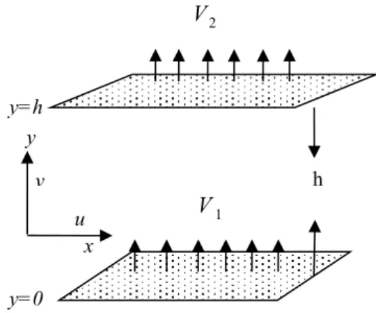
ORMULATION

The problem of two-dimensional steady laminar flow of an incompressible viscous couple stress fluid in a parallel porous channel is considered. Various types of flow occur and they fall under two

major categories: (i)

V

₁



V

₂ and (ii)

V

₂



V

₁ .

Fig. 1. Flow Geometry.

Based on the Stokes microcontinuum theory, the governing equations of the flow in the absence of body forces and body moments are the continuity equation and the momentum equations (Stokes 1966) given by

.

q

0

 

,

(1)



.



(

)

(

(

(

)))

q

q

p

q

q









      

        

.

(2)

The boundary conditions are

1 2

( , 0) 0 , ( , 0)

( , ) 0 , ( , )

u x v x V

u x h v x h V

 

  , (3)

and the no-couple stress conditions at the boundary are

2 2 2

2

0

at

0,

0

at

.

u

y

y

u

y

h

y











_

_



. (4)

Taking y

h



 , the above equations become

1

0

u

v

x

h





_



_





, (5)

2 2

2 2 2

1 1

u v u p u u

u

x h x x h



  

 

 _  _  _  _ 

 

 

   _  _,

y=h

y=0

h

1

V

2

V

y

4 4 4

4 4 4 2 2 2

1 2

u u u

x h h x



  

_{  } 

 _   _

   

  (6)

2 2

2 2 2

1 1

v v v p v v

u

x h h x x h

       _  _   _{ } _  _      _  _,

4 4 4

4 4 4 2 2 2

1 2

v v v

x h h x



  

_{  } 

 _   _

   

 

(7)

where p is the pressure and



is the kinematic

viscosity.

The boundary conditions are given by

1 2

( , 0) 0 , ( , 0) ,

( ,1) 0 , ( ,1) .

u x v x V

u x v x V

 

  (8)

and

2 2 2

2

0 at 0,

0 at 1.

u u









       

. (9)

Using a stream function (Berman, 1953) of the form

1 2

(0)

( , )

( )

(1)

(0)

(1)

(0)

V

V

hU

x

x s

s

s

s

s









_







_











, (10)

where

1

0

(0)

(0, )

U





u



d



is the entrance

velocity, the partial differential Eqs. (5)-(7) reduce to an ordinary differential equation.

Without loss of generality, it is assumed that

1 2

V



V

in the first case and

V

₂



V

₁ in the

second case.

2.1

Case(i)

V

₁



V

₂

The stream function of Eq.(10) in this case becomes

1 1

(0)

( , )x hU V x f( )









 

_  _

  , (11)

where ₁ 2

1

( )

( )

,

1

(0)

V

s

f

s

V













. (12)

Further, Eq. (6) and Eq. (7) respectively become



2



1 1 1 2 4 (0) 1 v V ff f V x

U h p

h _{f f} x

h h











 _{ }     _ _{ }    _    _  _   ,(13) 2 1 1 1 3 iv

V V p

f V ff f

h h



_





   

 , (14)

Eq.(14) is a function of



only and therefore

2

0 p x



 _

  . (15)

Using Eq.(15) in Eq.(13), a fifth order differential equation is obtained as

2 2

1( ) 1

v

l f  fR f  ff  A

, (16)

where

A

₁ is an arbitrary constant,

2 2 h l





 is the

dimensionless couple stress parameter and

1 1 /

R V h



is the Reynolds number. It may be

noted that Eq.(16) reduces to its Newtonian

counterpart when

l

2is made to vanish .

The boundary conditions from Eq. (8) and Eq. (9) become

1

(0)

1,

(0)

0,

(1)

1

,

(1)

0,

(0)

0,

(1)

0.

f

f

f

f

f

f









 













(17)

For the case of suction at the upper wall and

injection at the lower wall,



₁ takes the range

1

1  0

   and

R

₁



0

. For injection at the upper

wall and suction at the lower wall, the range is

1

1



0

   and

R

₁



0

. For suction at both walls,

it is required that

R

1



0,

 

2



1

 

1

, and for

injection at both walls, it is

R

₁



0,

 

2



₁

 

1

.

2.2

Case (ii)

V

₂



V

₁

In this case, the stream function becomes

2 2

(0)

( , )x hU V x g( )









 

_  _

  , (18)

where 1

2 2

1 V V



  and ( ) ( )

(1) s g s    .

Further Eq. (6) and Eq. (7) in this case reduce to



2



2 2 2 2 4 (0) 1 v V gg g V x

U h p

h x g g h h











 _{ }     _{ }       _     _{ }     ,(19) 2 2 2 2 3 iv

V V p

g V gg g

h h

 _ 

 

  

 . (20)

Eq.(20) is independent of

x

and therefore Eq.(15)

holds good in this case also. Using Eq. (15) in Eq. (19) as in case (i), a fifth order differential equation in ( )g is obtained as

2 2

2( ) 2

v

l g gR g gg A , (21)

where

A

₂is an arbitrary constant and

R

₂



V h

₂

/



is the Reynolds number in this case. Here again

Eq.(21) reduces to the Newtonian case when

l

2is

2

(0)

1

,

(0)

0,

(1)

1,

(1)

0, g (0)

0,

(1)

0.

g

g

g

g

g





 

















(22)

For the case of suction at the upper wall and

injection at the lower wall,



₂takes the range

2

0



1 and R₂0. For injection at the upper

wall and suction at the lower wall, the range of

values is 0



₂1 and R₂0. For suction at

both the walls, it is required that

2 0,

R 

1





2



2

and for injection at both the

walls, it is

R

₂



0,1





₂



2

.

3. S

OLUTION

O

F

T

HE

P

ROBLEM

3.1

Solution by DTM for Case (i)

Using differential transform about





0

, Eq. (16)

can be transformed into

1

1

2

1 1 1 1

0 1

1 1 1 1

0

1

(k 1)( 2)( 3)( 4)( 5) ( 5)

( 1)( 2)( 3) ( 3)

( 1)( 1) ( 1) ( 1)

( 1)( 2) ( ) ( 2)

( )

k

k

k

k

l k k k k F k

k k k F k

k k k F k F k k

R

k k k k F k F k k

A k

              _{     }                      





,(23)

and the first two boundary conditions and fourth condition from Eq. (17) are

(0) 1, (1) 0, (3) 0

F  F  F  . (24)

It is assumed that

F

(2)



b F

₁

,

(4)



d

₁ , where

1& 1

b

d

are undetermined constants. Using these

and Eq. (24) in Eq. (23), the values of F(k) are

obtained iteratively and the other three boundary conditions are written as

1 1

0

(1) 1 or ( ) 1

N

k

f



F k





 



  (25)

1 0

(1) 0 or ( 1) ( 1) 0

N

k

f k F k





 



   (26)

3 0

(1) 0 or ( 1)(k 2)(k 3) ( 3) 0

N

k

f k F k





 



     (27)

For N=17, solving the three Eqs. (25), (26) and (27), the values of

b d

₁

,

₂ and

A

₁are obtained.

Using Eqs. (13) and (14), the general expression for pressure distribution is obtained as

2

2 2

1 1

2

1 1 1

3 2

1

( , )

(0, 0)

( )

( )

(0)

2

(0)

( )

2

p x

p

V

V

f

f

f

h

V

A

U

V

x

f

x

h

h

h





_



_



_

















_



_











_



_





,(28)

From this general expression the pressure

distribution for x and  directions are deduced. The

non- dimensional pressure drop in the x and 

directions are respectively given by

 

2

1 1

* 1

(0, )

( , )

(0) / 2

1

1

2

8

x

p

p x

p

U

x

A

h

R





















_



_





, (29)





2 2 2 2 2 1 1 * * 2 2 1 *

( ,0) ( , ) (0) / 2

4 4

( ) (1) 2 ( )

4

( ) (0) p x p x

p

U R

f R f

R R

R l f f R           _{ }  _{ } _{  }  _ _{ }       _{ } _{ }    . (30)

where 1

1 *

R x h R



 is a non-dimensional variable

and

R

*



4

hU

(0) /



is the entrance Reynolds number.

The non-dimensional stream function is given by

1 1

( , ) 1

( , ) 4 ( )

(0)

x

x

f

hU













    _  _   . (31)

The skin friction is defined as

2 2

2 ( / )

(0) / 2 hU(0)

wall wall f u c U











 

  , (31)

where τwall is the shear stress at the wall and the skin friction here becomes

1 1

1 1

8 1

4 [ ( )]

f wall

h

c

f

R x









 



 _  _

  . (32)

3.2

Solution by DTM for Case (ii)

In this case, Eq. (21) is transformed to

1

1

2

1 1 1 1

0 2

1 1 1 1

0

2

( 1)( 2)( 3)(k 4)(k 5) ( 5)

( 1)( 2)( 3) ( 3)

( 1)( 1) ( 1) ( 1)

( 1)( 2) ( ) ( 2)

( )

k

k

k

k

l k k k G k

k k k G k

k k k G k G k k

R

k k k k G k G k k

A k

              _{     }                      





,(33)

and the first two boundary conditions and fourth condition from Eq. (22) are

2

(0) 1 , (1) 0, (3) 0

G  



G  G  . (34)

It is assumed that

G

(2)



b

₂

,

G

(4)



d

₂, where

2, d2

b

are undetermined constants. Using these and

Eq. (34) in Eq. (33), the values of G(k) are obtained

0

(1) 1 or ( ) 1

N

k

g G k







 (35)

1 0

(1) 0 or ( 1) ( 1) 0

N

k

g k G k





 



   (36)

3 0

(1) 0or ( 1)(k 2)(k 3) G( 3) 0

N

k

g k k





 



     (37)

For N=17, solving the three equations (35),(36) and (37), the values of

b

₂

, d

₂ and

A

₂are obtained. Using (19) and (20), the general expression for pressure distribution in this case is obtained as

2

2 2

2 2

2

1 2 2

3 2

2

( , ) (0, 0)

( ) ( ) (0)

2 (0) g ( )

2

p x p

V V

g g g

h

V A U V x

x h

h h



 _  _

 _ 

 

  

  _  _

 



  _  _

 

, (38)

From this general expression, the pressure

distribution for x and  directions are deduced. The

non-dimensional pressure drop in the x and

directions are respectively given by





2 2

* 2

1 1

2 8

x x

p A

h

R  

   _  _

 

,

(39)





2

2 2

2

2

2 2

2

2 * * 1

4

( ) (1 )

*

4 4

2 ( ) g ( ) (0)

R

p g

R

R g R l g

R R

  

 

 _{  }

_{  }   _

 

  _   _{ }

 _{ } _{ } 

   

.(40)

where ₂

R x

2_*

h

R



 is a non-dimensional variable.

In this case, the non-dimensional stream function and the skin friction are given by

2 2

( , )

1

( , )

4

( )

(0)

x

x

g

hU























_



_





& (41)

2 2

2 2

8 1

4 [ ( )]

f wall

h

c

g

R x









  _

 _  _

  . (42)

4. R

ESULTS

A

ND

D

ISCUSSION

The problem of a steady, two-dimensional laminar flow of couple stress fluid in a porous channel has been solved using DTM under two cases (i)

V

₁



V

₂ and (ii)

V

₂



V

₁ .

In case (i),

R

₁is taken to be positive and the values

of wall permeability



₁ 0.2, 0.6 correspond

to suction at the upper wall and injection at the

lower wall, that of



₁ 1correspond to a solid

upper wall and injection at lower wall and those of

1 1.4, 1.8



   correspond to injection at both the

walls. Other cases of suction at both walls, injection

at upper wall and suction at lower wall correspond

to negative values of R₁. In particular,

V

₂0in

case (i) reduces to the problem of Kabadi (1987).

Figures 2-8 correspond to the results of case (i).

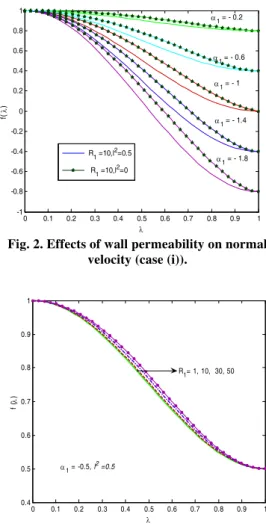
Fig. 2 shows the effects of 1onnormal velocity

for the Reynolds numberR₁10, couple stress

parameter _l2_{= 0.0 & 0.5}

and for different values of

the wall permeability parameter

α

₁.

0 0.1 0.2 0.3 0.4 0.5 0.6 0.7 0.8 0.9 1

-1 -0.8 -0.6 -0.4 -0.2 0 0.2 0.4 0.6 0.8 1



f(



)

R₁ =10,l2=0.5

R₁ =10,l2=0

₁ = - 0.2

₁ = - 0.6

₁ = - 1

1 = - 1.4

₁ = - 1.8

Fig. 2. Effects of wall permeability on normal velocity (case (i)).

0 0.1 0.2 0.3 0.4 0.5 0.6 0.7 0.8 0.9 1

0.4 0.5 0.6 0.7 0.8 0.9 1

 f (

)

R

1= 1, 10, 30, 50

₁ = -0.5, l2 =0.5

Fig. 3. Effects of inertia on normal velocity (case (i)).

0 0.1 0.2 0.3 0.4 0.5 0.6 0.7 0.8 0.9 1 0.5

0.55 0.6 0.65 0.7 0.75 0.8 0.85 0.9 0.95 1



f(



)

R₁=50, 1= -0.5

l2=0.8,0.6,0.4,0.2,0

0 0.1 0.2 0.3 0.4 0.5 0.6 0.7 0.8 0.9 1 -3

-2.5 -2 -1.5 -1 -0.5 0 0.5



f ' (



)

R₁=10, l2=0.5 R₁=10, l2=0

₁= - 0.2

₁= - 0.6

₁= - 1

₁= - 1.4

₁= - 1.8

Fig. 5. Effects of wall permeability on axial velocity (case(i)).

0 0.1 0.2 0.3 0.4 0.5 0.6 0.7 0.8 0.9 1 -0.8

-0.7 -0.6 -0.5 -0.4 -0.3 -0.2 -0.1 0 0.1



f '

(

)

R₁= 1, 10, 30, 50

₁= - 0.5, l2= 0.5

Fig. 6. Effects of inertia on axial velocity (case (i)).

0 0.1 0.2 0.3 0.4 0.5 0.6 0.7 0.8 0.9 1

-0.9 -0.8 -0.7 -0.6 -0.5 -0.4 -0.3 -0.2 -0.1 0 0.1



f ' (



)

R₁=50, 1= -0.5

l2=0.8,0.6,0.4,0.2,0

Fig. 7. Effects of couple stresses on axial velocity (case (i)).

Here _l2_{= 0.0}

correspond to the Newtonian case. The normal velocity decreases with increase in

magnitude of1. Also, the effect of couple stresses

2_{= 0.5}

l on the flow behavior is to further decrease

the normal velocity. Fig. 3 shows the inertia effects

on normal velocity for



₁0.5,l20.5 and

different values of R₁. It is observed that the

normal velocity increases with increasing Reynolds number.

Figure 4 shows the effects of couple stresses on the normal velocity. The normal velocity component decreases throughout the domain for increasing values of the couple stress parameter as

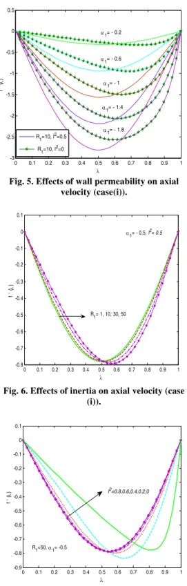
seen in Fig. 2. Fig. 5 gives the effects of 1on

axial velocity for 2

1 10, 0.0 & 0.5

R l  and different values of 1.

2

0.0

l  corresponds to the

Newtonian case where the axial velocity profiles

are skewed close to the upper wall. For 2

0.5 l  ,

increase in magnitude of 1increases the

magnitude of axial velocity, with minimum magnitudes at both walls and maximum magnitudes near the middle of the wall. Thus couple stresses are seen to permit a smooth flow. Fig. 6 shows the inertia effects on axial velocity

for



₁





0.5,

l

2



0.5

and for different values of

1

R. It is observed that the axial velocity decreases

in magnitude as the value of R₁is increased up to

a certain value of



. Above this value, the

velocity increases in magnitude due to increase in

lower wall velocity V₁ which is greater than upper

wall velocity V₂.

The effects of couple stresses on axial velocity are shown in Fig. 7. It can be seen that the axial velocity decreases for increasing couple stress parameter near the lower wall and the trend is reversed near the upper wall. Here, it is clearly seen that the flow becomes smoother as the couple stress

parameter increases froml2 0.0 to l2 0.8.

Fig. 8 shows the pressure drop in axial direction for various values of Reynolds number and for various values of couple stress parameter. The pressure drop decreases with decreasing Reynolds number and with decreasing couple stress parameter.

0 50 100 150 200 250 300 350 400 0

2000 4000 6000 8000 10000 12000 14000

x/h

Px

R₁=1, l2= 0.5

R₁=10,l2= 0.5

R1=50,l

2_{= 0.5} R₁=50,l2= 0.8

1= -0.5

Fig. 8. Axial pressure drop (case (i)).

Similar graphs are plotted for case (ii) in Figs.

values of



₂ 0.2, 0.6 correspond to suction at the upper wall and injection at the lower wall,

that of



₂ 1 correspond to a solid lower wall

and suction at upper wall and those of

2 1.4,1.8



 correspond to suction at both walls.

Other cases of injection at both walls, injection at upper wall and suction at lower wall correspond

to negative values of

R

₂. Fig. 9 shows the effect

of



₂ on normal velocity for the Reynolds

number R₂10, couple stress parameter

2

0.0 & 0.5

l



and for different values of the

wall permeability parameter



₂. The normal

velocity decreases as the value of



₂ decreases

for l2 0.5. Also, the effect of couple stresses

on the flow behavior is to further decrease the normal velocity. Fig. 10 shows the inertia effects

on normal velocity for



₂ 0.5,l2 0.5and

different values of

R

₂. It is observed that the

normal velocity decreases with increasing Reynolds number.

Figure 11 shows the effects of couple stresses on the normal velocity. The normal velocity decreases with decrease in couple stress

parameter. Fig. 12 gives the effects of 2onaxial

velocity for R₂ 10,l2 0.0 & 0.5 and different

values of



₂. l2 0.0 corresponds to the

Newtonian case where the axial velocity profiles

are skewed close to the upper wall. Forl20.5,

increase in



₂ increases the axial velocity, with

minimum values at both walls and maximum values near the middle of the wall. Thus couple stresses are seen to admit a smooth flow. Fig. 13 shows the effects of inertia on axial velocity

profile for



₂ 0.5,l20.5 and different

values of

R

₂. It is observed that the axial

velocity decreases as the value of

R

₂ increases

up to a certain value of



. Above this value, the

velocity increases due to increase in

V

₂which is

greater than

V

₁. The effects of couple stresses on

the axial velocity for fixed values of

2 2 10, 0.5

R  l  are shown in Fig. 14. The axial

velocity is increasing with increasing couple

stress parameter for certain values of



and after

that it is decreasing. Here, it is clearly seen that the flow becomes smoother as the couple stress

parameter increases froml2 0.0 to l2 0.8. In

Figs. 11 and 14, when the couple stress parameter is equal to zero, it represents the Newtonian fluid case. Fig. 15 shows the pressure drop in axial direction for various values of Reynolds number and for various values of couple stress parameter. The pressure drop decreases with increasing Reynolds number and with increasing couple stress parameter.

0 0.1 0.2 0.3 0.4 0.5 0.6 0.7 0.8 0.9 1

-0.8 -0.6 -0.4 -0.2 0 0.2 0.4 0.6 0.8 1 1.2



f(

)

R₂=10,l2_=0.5

R₂=10,l2₌₀ 2=0.2

2=1.4

2=1

2=0.6 2=1.8

Fig. 9. Effects of wall permeability on normal velocity (case (i)).

0 0.1 0.2 0.3 0.4 0.5 0.6 0.7 0.8 0.9 10

0.5 0.6 0.7 0.8 0.9 1 1.1



f (

)



2=0.5, l

2

= 0.5

R₂= 1,10,30,50

Fig. 10. Effects of inertia on normal velocity (case (ii)).

0 0.1 0.2 0.3 0.4 0.5 0.6 0.7 0.8 0.9 1

0.5 0.6 0.7 0.8 0.9 1 1.1 1.2



f(



)

R₂=50, ₂=0.5

l2_{= 0.8,0.6,0.4,0.2,0}

Fig. 11. Effects of couple stresses on normal velocity (case (ii)).

0 0.1 0.2 0.3 0.4 0.5 0.6 0.7 0.8 0.9 1

-0.5 0 0.5 1 1.5 2 2.5 3



f ' (



)

R₂=10, l2_=0.5

R₂=10, l2=0

₂=0.2

₂=0.6

₂=1

₂=1.4

₂=1.8

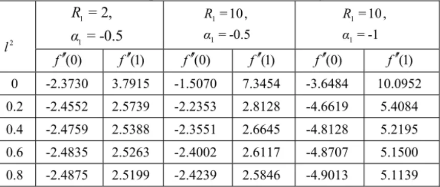
Table 1 Effects of couple stresses on skin friction by DTM – case (i)

2

l

1 1

= 2,

= -0.5

R

α

=-0.5

, 10 =

1 1 α R

1 -=

, 10 =

1 1 α R

) 0 (

′ ′

f f′′(1) f′′(0) f′′(1) f′′(0) f′′(1) 0 -2.3730 3.7915 -1.5070 7.3454 -3.6484 10.0952

0.2 -2.4552 2.5739 -2.2353 2.8128 -4.6619 5.4084

0.4 -2.4759 2.5388 -2.3551 2.6645 -4.8128 5.2195

0.6 -2.4835 2.5263 -2.4002 2.6117 -4.8707 5.1500

0.8 -2.4875 2.5199 -2.4239 2.5846 -4.9013 5.1139

Table 2 Effects of couple stresses on skin friction by DTM – case (ii).

2

l

2

2

= 2,

= 0.5

R

α

= 0.5

, 10 =

2 2 α R

1 =

, 10 =

2 2 α R

) 0 (

′ ′

g g′′(1) g′′(0) g′′(1) g′′(0) g′′(1) 0 2.3466 -3.9354 1.1486 -10.388 1.6085 -19.770

0.2 2.4550 -2.5740 2.2211 -2.8274 4.6159 -5.4668

0.4 2.4758 -2.5389 2.3509 -2.6692 4.8009 -5.2350

0.6 2.4835 -2.5264 2.3983 -2.6141 4.8655 -5.1572

0.8 2.4875 -2.5200 2.4228 -2.5860 4.8997 -5.1157

0 0.1 0.2 0.3 0.4 0.5 0.6 0.7 0.8 0.9 1 0

0.1 0.2 0.3 0.4 0.5 0.6 0.7 0.8



f '

(

)

₂=0.5,l2=0.5

R₂=1,10,30,50

Fig. 13. Effects of inertia on axial velocity (case (ii)).

Tables 1 and 2 present comparisons between

Newtonian (l20) and non-Newtonian results

(l20), revealing the effects of couple stresses

on the skin friction in case (i) and case (ii) respectively. From Table 1 of case (i), it is observed that the magnitude of skin friction increases at the lower wall and decreases at the upper wall with an increase in couple stress

parameter for all values of

α

₁ &

R

₁. Here,

1

= -0.5

α

corresponds to the case of one wall

injection and other wall suction, whereas

α

₁

= -1

corresponds to the case of solid upper wall and injection at the lower wall. Further, the magnitude of the skin friction decreases at the

lower wall whereas it increases at the upper wall with an increase in Reynolds number for fixed values of

α

1 and l

2 _.

0 0.2 0.4 0.6 0.8 1

-0.1 0 0.1 0.2 0.3 0.4 0.5 0.6 0.7 0.8 0.9



f '

(

)

R₂=50, ₂=0.5

l2= 0.8,0.6,0.4,0.2,0

Fig. 14. Effects of couple stresses on axial velocity (case (ii)).

From Table 2 of case (ii), it is observed that the magnitude of skin friction increases at the lower wall and decreases at the upper wall with an increase in couple stress parameter for all values of

α

₂ &

R

₂as in case (i). In Table 2

α

₂

= 0.5

corresponds to the case of one wall injection and

other wall suction, whereas

α

₂

= 1

corresponds

increases at the upper wall with an increase in

Reynolds number for fixed values of

α

₂ and l2_.

Thus the effect of couple stresses on the magnitude of skin friction in both cases gets enhanced at one wall and diminished at the other wall.

0 50 100 150 200 250 300 350 400

-3500 -3000 -2500 -2000 -1500 -1000 -500 0 500

x/h

Px

R 2=1, l

2 _=0.5

R 2=10, l

2 _=0.5

R₂=50, l2 =0.5

R₂=50, l2 =0.8

₂= 0.5

Fig. 15. Axial pressure drop (case(ii)).

5. C

ONCLUSION

In this paper, differential transform method is used successfully for finding the solution of two dimensional steady laminar flow of an incompressible couple stress fluid in a porous channel. It is seen that this method is simple and easy to use and solves the problem without any discretization and does not require exertion of any flow parameter as in perturbation method. Although the non-Newtonian fluid flow problem deals with more complicated governing equations than the Newtonian case, the method does not get disturbed and works well. Besides this, the reliability of the method and reduction in size of computational domain gives this method a wider applicability. Hence, the Differential Transform Method is an effective and reliable tool in finding the semi- analytical solution to many non-linear systems. This paper uses DTM for the flow problem with the couple stress model of the non-Newtonian fluid. However, there is no limitation for applying the DTM for such problems in similar geometry with any other non-Newtonian fluid model.

R

EFERENCES

Ariel, P. D. (2002). On exact solutions of flow problems of a second grade fluid through two

parallel porous walls. Int. J. Eng. Sci. 40,

913-941.

Berman, A. S. (1953). Laminar flow in channels

with porous walls. Journal of. Applied. Physics

24, 1232-1235.

Bert, C. W. (2002). Application of differential transform method to heat conduction in

tapered fins. Journal of Heat Transfer 124,

208-209.

Chen, C. K. and S. H. Ho (1999). Solving partial differential equations by two dimensional

differential transform method. Applied

Mathematics and Computation 106, 171-179. Erturk, V. S., S. Momani (2007). Differential

transform method for obtaining positive solutions for two-point nonlinear boundary

value problems. International Journal:

Mathematical Manuscripts 1(1), 65-72. Kabadi, A. S. (1987). The influence of couple

stresses on the flow of fluid through a channel

with injection. Wear 119, 191-198.

Kamsili, F. (2006). Laminar flow of a non-Newtonian fluid in channels with wall suction or injection. Int. J. Eng. Sci. 44, 650-661 Kurnaz, A., G. Oturanc and M. E. Kiris (2005).

n-dimensional differential transform method for

PDE. International Journal of Computer

Mathematics 82(3), 369-380.

Rashidi, M. M. and S. M. Sadri (2010). Solution of the laminar viscous flow in a semi-porous channel in the presence of a uniform magnetic field by using the differential transform

method. Int. J. Contemp. Math. Sciences 5(15),

711-720.

Rashidi, M. M. and E. Erfani (2011). The Modified Differential Transform Method for Investigating Nano Boundary-Layers over

Stretching Surfaces. International Journal of

Numerical Methods for Heat and Fluid Flow

21(7), 864-883.

Rashidi, M. M. and S. A. Mohimanian Pour (2010). A Novel Analytical Solution of Heat Transfer of a Micropolar Fluid through a Porous

Medium with Radiation by DTM-Padé. Heat

Transfer-Asian Research 39(8), 575-589. Rashidi, M. M., S. A. Mohimanian Pour and N.

Laraqi (2010). A semi-analytical solution of micro polar flow in a porous channel with mass injection by using differential transform

method. Nonlinear Analysis: Modeling and

Control 15(3), 341-350.

Srinivasacharya, D, N. Srinivasacharyulu and O. Ojjela (2009). Flow and heat transfer of couple stress fluid in a porous channel with expanding

and contracting walls. International

Communication in Heat and Mass Transfer

36(2), 180-185.

Srinivasacharya, D, N. Srinivasacharyulu and O. Ojjela (2010). Flow of Couple Stress Fluid Between Two Parallel Porous Plates.

International Journal of Applied Mathematics

41(2), 10-14.

Stokes, V. K. (1966). Couple Stresses in Fluids.

Phys. Fluids 9, 1709- 1715.

Terrill, R. M. (1964). Laminar flow in a uniformly

porous channel. The Aeronautical Quarterly

Terrill, R. M. and G. M. Shrestha (1965). Laminar flow through parallel and uniformly porous

walls of different permeability. ZAMP 16,

470-482.

Vimala, P. and P. Blessie Omega (2013). Laminar flow of a Newtonian fluid through parallel porous walls solution by differential transform

method. In Proceedings of the Fortieth

National Conference on Fluid Mechanics and

Fluid Power 1549-1558.

Yuan, S. W. (1956). Further investigation of laminar flow in channels with porous walls.

Journal of Applied Physics 27, 267-269.

Zhou, J. K. (1986). Differential transformation and