www.geosci-model-dev.net/5/1061/2012/ doi:10.5194/gmd-5-1061-2012
© Author(s) 2012. CC Attribution 3.0 License.
Geoscientific
Model Development
A community diagnostic tool for chemistry climate model validation
A. Gettelman1, V. Eyring2, C. Fischer1, H. Shiona3, I. Cionni2, M. Neish4, O. Morgenstern3, S. W. Wood3, and Z. Li1
1National Center for Atmospheric Research, Boulder, CO, USA
2Deutsches Zentrum f¨ur Luft- und Raumfahrt (DLR) Institut f¨ur Physik der Atmosph¨are, Oberpfaffenhofen, Germany 3National Institute for Water and Atmosphere Research, New Zealand
4University of Toronto, Toronto, ON, Canada
Correspondence to:A. Gettelman ([email protected])
Received: 18 April 2012 – Published in Geosci. Model Dev. Discuss.: 11 May 2012 Revised: 16 July 2012 – Accepted: 2 August 2012 – Published: 3 September 2012
Abstract. This technical note presents an overview of the Chemistry-Climate Model Validation Diagnostic (CCMVal-Diag) tool for model evaluation. The CCMVal-Diag tool is a flexible and extensible open source package that facili-tates the complex evaluation of global models. Models can be compared to other models, ensemble members (simula-tions with the same model), and/or many types of observa-tions. The initial construction and application is to coupled chemistry-climate models (CCMs) participating in CCMVal, but the evaluation of climate models that submitted output to the Coupled Model Intercomparison Project (CMIP) is also possible. The package has been used to assist with analysis of simulations for the 2010 WMO/UNEP Scientific Ozone As-sessment and the SPARC Report on the Evaluation of CCMs. The CCMVal-Diag tool is described and examples of how it functions are presented, along with links to detailed de-scriptions, instructions and source code. The CCMVal-Diag tool supports model development as well as quantifies model changes, both for different versions of individual models and for different generations of community-wide collections of models used in international assessments. The code allows further extensions by different users for different applications and types, e.g. to other components of the Earth system. User modifications are encouraged and easy to perform with min-imum coding.
1 Introduction
The future evolution of ozone, climate and air quality are coupled and depend on interactions between atmospheric chemistry, dynamics, and radiation (Brasseur and Roeckner,
This technical note documents a diagnostic package for CCMs, the Chemistry Climate Model Validation Diagnos-tic (CCMVal-Diag) tool. The CCMVal-Diag tool facilitates comparisons between models, and between models and ob-servations. The diagnostic tool is an integrated part of the larger international CCMVal effort to improve model repre-sentations of stratospheric chemistry and climate (SPARC-CCMVal, 2010).
The CCMVal-Diag code is open source, extensible and flexible. In principle, the code is generic, and new variables representing other parts of the Earth system can easily be an-alyzed. It can analyze multiple models (where “model” is a given code used for a simulation) or multiple ensembles of a single model (using the same code). The code can produce performance metrics and is designed to enable comparison of models to observations. Examples are shown for global grids, but any gridded output (for example from limited area regional models) can be analyzed in the same way. It is de-signed to be easy for a user to modify and customize the tool. The current version of the diagnostic tool (version 3) is designed to convert model output to the Climate and Fore-cast (CF) metadata compliant CCMVal-2 data standard (see Sect. 2.2) and to produce standard diagnostics. More in-formation about the CCMVal-2 data standard is provided through links in Appendix A. This version specifically works with CCMVal-2 model output, but also will process the out-put used for the Coupled Model Intercomparison Project (CMIP) versions 3 and 5. The CCMVal-Diag tool has been used for analysis of CCMs in the SPARC-CCMVal (2010) report and World Meteorological Organization (2010) Scien-tific Assessment of Ozone Depletion.
This technical note is organized as follows. A basic code description is provided in Sect. 2. Section 3 describes how to run and modify the tool. Some examples of how the tool can be used for developing simple and complex diagnostics for global chemistry and climate models compared to observa-tions and each other are presented in Sect. 4, and a summary in Sect. 5. The CCMVal-Diag tool source code, observational data sets and links to model output are available via the web-site listed in the Appendix. A more detailed set of instruc-tions for installing and running the tool, as well as versioning and references, is available in a “readme” file in the source code distribution.
2 CCMVal-Diag structure
2.1 Principles
Several overall principles have guided the development of the CCMVal-Diag tool. The code is designed to compare models to each other and to observations. The purpose is to elevate the standard of process-oriented evaluation of global models, particularly chemistry-climate models, over time. The diag-nostics should be traceable: the code is kept in an archive,
and users are encouraged to upload (see Appendix A) their own diagnostics and improvements to existing diagnostics, to become part of the tool. Diagnostics should be repeatable as new models (or versions of models) are developed or new observations are added. Observations enter the tool in a pro-cessed manner, and multiple observations for the same diag-nostic or species can be included. The tool is modular and extensible: it can be used to run a single diagnostic or many diagnostics. Diagnostics can be as simple as direct translation of model output, to highly derived and calculated quantities based on multiple variables. The version of the diagnostic tool described here will process output at any time frequency, but is designed for monthly time series.
The tool is based on a minimal set of open source packages available on many platforms. The CCMVal-Diag code is de-signed so that users can edit (hack) the tool with minimum programing experience, by following examples.
2.2 Basic description
The CCMVal-Diag code is based on Python and the National Center for Atmospheric Research (NCAR) Command Lan-guage (NCL) scripting lanLan-guage. It requires these two pack-ages to be installed (see Sect. 2.3). It takes as input either (a) raw model output or (b) Network Common Data For-mat (NetCDF) files in CCMVal-2 data request forFor-mat (Eyring et al., 2008). If (a), it can process model output into (b) with code written for a specific model (see Sect. 3.1). CCMVal-2 data format is CF compliant with standard variable names. The CCMVal-2 standard differs in that it adds some addi-tional metadata and coordinate descriptions (such as time and date arrays) not required by CF.
The tool can be used to convert “raw” model output to CF compliant output. Customization is required for each model to get output into the CF format. This initial release comes with code for translating NCAR Community Climate Sys-tem Model (CCSM) format NetCDF files as a Sys-template. Each model will need its own piece of code to do this.
The code will read files compliant with the CF NetCDF CCMVal-2 format. However, there are some models with slightly incompatible formats due to improper use of the specification. An example might be an offset in the time di-mension, or the wrong units for the pressure field. A flexible mechanism in the code allows model-specific changes to be added easily as they are discovered, by adding a function to fix data for a specific model and project (CCMVal2, CMIP5). CCMVal-2 model output is available from the British Atmo-spheric Data Center (BADC). For more details about obtain-ing CCMVal-2 model data, see the links in Appendix A.
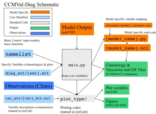
main.py
namelist
Model Output
(netCDF)
Climatology &
Timeseries netCDF Files
(CCMVal-CF compliant)
diag_att/[set].att
Plot variables
(netCDF)
Figures
(PNG/GIF/EPS)
Observations (Climo)
var_att/[var]_att.ncl plot_type/
(loop over variables)
[model_name].py
Basic Control: input models, basic functions
Model specific read code
Specify Variables (climatologies) & plots
Variable descriptions (computation)
(named in [set].att) Plotting codes (named in [set].att) Model Specific
User Modified Standard Code Output Observations
reformat/[model]_convert.txt
Model specific variable mapping
[model_name].ncl
CCMVal-Diag Schematic
Fig. 1. Schematic figure depicting the operation of the CCMVal-Diag tool as described in the text.
The code will further create climatology and time series files for the specified variables, and create publication quality (postscript) figures. Figures 2 through 8 were produced with the tool.
The operation of the tool is illustrated schematically in Fig. 1. The basic control is in Python. Python is used as a scripting layer to parse namelists and call NCL code. NetCDF file input/output, variable manipulation and plotting are all handled by NCL, requiring no extra libraries or con-figuration. The basic operation is to call the main Python routine and pass it a namelist file. The namelist specifies (a) global flags, (b) model output to process and (c) a file of diagnostic sets to run. The diagnostic sets (diag att/[set].att) specify the diagnostics to pro-cess.
A “diagnostic” in the CCMVal tool has two compo-nents: avariable([var])and aplot (plot type) rou-tine. Variable descriptions are contained in a variable at-tributes directory (var att). New variables are placed here as well. The code looks for a variable attribute file (var att/[var] att.ncl). Variable names are either standard names from the CCMVal-2 CF specification, or “derived” variables. Derived variables are functions of other variables. Each variable name must have a variable attribute file. The variable attribute file contains NCL code for pro-cessing derived variables. This can be as simple as chang-ing units (e.g. multiplychang-ing by a constant or field), or a combination of other variables. For example, the lapse rate tropopause temperature (or other properties) can be calcu-lated based on a set of temperature profiles. The variable
attribute file also sets attributes used to run different plotting routines for the variable (for example, defining a text name and units, and contour intervals). These attributes are used by specific plotting routines.
The second component of a diagnostic is a plotting routine. The plotting routines are NCL routines in theplot type directory. For the example of the tropopause temperature cited above, it can be plotted in many ways: a zonal mean, a trend in some region or season over time, a map of the temperature or a map of trends, etc. These “plot types” are discussed in Sect. 4. Specific plotting attributes, such as axis ranges or contour intervals, can be specified in the variable attributes file for each variable and plot type. The diagnos-tic code can send the inputs to a plotting routine, or save a processed variable to a file in a standard format. For exam-ple, tropopause temperature can be saved to a CCMVal-2 CF compliant NetCDF file that looks like any other input vari-able to the diagnostics so that computation needs only occur once.
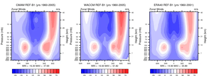
Fig. 2. Zonal mean zonal wind averaged for 1980–1990 from two historical (REF-B1) model simulations (left and center) included in the CCMVal-2 archive and ERA40 reanalyses (right). Models are the Canadian Middle Atmosphere Model (CMAM-Left) and the Whole Atmosphere Community Climate Model (WACCM-Center). The height values are a logarithmic interpolation from standard atmosphere of the pressure.
(latitude-longitude) and z=zonal mean (latitude-level).
For example, a zonal monthly mean time series is indi-cated as T2Mz (T=timeseries, 2=number of dimensions,
M=monthly mean, z=zonal mean). Monthly means of
a 3-D variable (latitude, longitude, altitude) are indicated as T3M. Once the variable is processed for each model, a standard data structure is passed to the plotting routines in theplot typedirectory. These routines produce graphics and standard output (such as trend calculations or perfor-mance metrics) as well as have the option to produce files containing the data on the plot (noted as “Plot variables” in Fig. 1).
The code is set up to read in NetCDF files with either one time sample per file or multiple time samples per file. It can also concatenate variables across multiple files. Examples of reading one and multiple time samples per file are contained in the sample read code for CCSM.
2.3 Installation
The CCMVal-Diag tool has been designed to use a minimum of open source packages, and no proprietary software. In-stallation of the code requires only Python and NCL. The CCMVal-Diag tool requires basic Python for the driver layer (Fig. 1). The code has been tested with Python version 2.3.4 and should run with 2.3.4 or later. Python source code and bi-naries for most systems are available from the Python project (www.python.org).
The CCMVal-Diag tool uses NCL for most of its process-ing (manipulatprocess-ing NetCDF files) and for preparprocess-ing graphics. NCL is also an open source package, with binaries for many systems (AIX, IRIX, Linux, MacOSX, Solaris, Windows).
The code requires NCL version 5.1.0 or later (www.ncl.ucar. edu).
2.4 Observations
Comparisons between simulations and observations are a critical part of model evaluation, and the CCMVal-Diag tool has been designed to easily incorporate observations in quali-tative and quantiquali-tative evaluation. Observations enter the tool in two ways: either as another “model” or as a separate plot-specific data file.
In the first method, observations can be converted into a format identical to the models. This can be done if the obser-vations are available in gridded format for a defined time pe-riod. Reanalyses are the most common type of such “obser-vations”, or long-term or multi-satellite records. Several ex-amples of such observations are shown in Sect. 4 (e.g. Fig. 2). In these cases, the observations are listed in the namelist as another model.
Another method is to tailor observations for specific com-parisons. In this method, often a climatology from a specific observation type is processed for a specific type of plot, and written in theplot typecode. Such observations are spec-ified as attributes for a specific variable, usually for a specific plot type. This method is also illustrated in Sect. 4 (Figs. 7 and 8; see below).
3 Processing methods
In this section, we describe the different processing methods that the CCMVal-Diag tool provides, and ways to use the tool.
3.1 Converting model output
In general, global models write data sequentially, with many variables for individual time samples, in files with single or multiple time samples. For intercomparison projects, typi-cally files with multiple time samples and a single variable are desired to reduce output size, and for ease of processing. The CCMVal-Diag tool provides a framework and examples for processing of model output into correct formats for inter-comparisons. It can also be used to check formatting conven-tions. Currently, the most commonly used format is the CF compliant NetCDF standard, and the tool is designed to read this (and optionally write).
The CCMVal-Diag tool will process model output and generate two types of files: time series files (T3M, T2Ms, etc) which contain one variable at all times. The type specifica-tion follows the CCMVal-2 convenspecifica-tion described earlier. The code also makes “climatology files” (C3M, etc) that are used internally for plotting, or in further post-processing. Time-series files are in CCMVal-2 CF compliant NetCDF format.
For processing of model files, the code requires 3 files (or-ange in Fig. 1): (a) a Python driver to find the files, (b) an NCL code to process the files and (c) a text file to remap model variable names to CF compliant CCMVal-2 format variable names. The Python code (modelname.py) sets the filenames, gets the variable names, and then calls the NCL processing code (modelname.ncl). The NCL pro-cessing code performs operations on the file list to concate-nate files together. For the initial conversion implementa-tion with the NCAR CCSM, the raw model output files are NetCDF files, but the structure will work on any other file type that NCL can read. The user can supply NCL code to read a specific raw model output in any format (binary, GRIB, HDF, ASCII, etc), and the tool will then process the files to CF compliant format. A utility for checking CF com-pliance is also included in the tool.
3.2 Comparing models to observations
Model comparisons to observations use one of the two meth-ods described in Sect. 2. Basically, these methmeth-ods involve pre-processing the data to be interpreted as a separate model, or further processing to produce data directly for plotting. An example of the first type, data processed like a model, might be for a gridded satellite product, where 2-D (zonal or a surface) or 3-D monthly means can be produced in the CCMVal-2 format. Another example is a reanalysis data set such as the ERA40 reanalysis (Uppala et al., 2005) shown in Fig. 2. Further examples are shown in Sect. 4. The second
type would be a more heavily processed data set, read in for a specific variable and a specific plot. This could be an an-nual climatology file (monthly climatology of water vapor in 2-D or 3-D), such as used from the HALOE satellite in Fig. 7. The diagnostic tool can even use specific values of a derived product (for example, meridional heat flux, defined as the product of anomalies of zonal wind (v′) and
temper-ature (T′)). These multiple methods allow flexibility. Both
methods could be used in common for the same variable.
3.3 Comparing models to each other
In addition to comparing models to observations, the CCMVal-Diag tool is designed to compare models to each other. The number of models is arbitrary. Model names (and a standard set of colors and line styles) for CCMVal mod-els have been included in the CCMVal-Diag tool, but modmod-els without a known name will still be processed. The names and number of models are simply read from the namelist. Each run or ensemble member is treated separately. Mul-tiple ensemble members from a single model can be pro-cessed. Each ensemble member can have different start and end dates. Some diagnostics require full years for process-ing. Many diagnostics can take a “reference” model (or ob-servation) for difference plots. Model output from different scenarios can be placed on the same plot, such as a historical run and a future scenario, or two different future scenarios. The standard CCMVal-2 model set contains up to 18 models, some with ensemble members available.
Models can have their own grids (e.g. Fig. 3). In principle, models need not have a full global grid either (limited area models can be processed). Difference plots interpolate and regrid for comparison purposes.
3.4 Quantitative trends and performance metrics
Several of the plotting routines are designed to plot time se-ries, and these plots also produce quantitative estimates of trends. Trends can be calculated using any method desired. Currently, several of the routines provide trends based on linear regression with significance testing, providing quanti-tative trends as well as confidence intervals. Trends can also be used as a diagnostic, for example plotting trends on a map (see Sect. 4).
Fig. 3. Contour plot of June–August surface air temperature (K) for “historical” (AMIP) runs from three models that are part of CMIP5. Averages are from 1980–2005 for the Norwegian Earth System Model (NorESM), the Centre National de Recherches M´et´eeorologiques Model (CNRM-CM5) and the model of the Institut Pierre Simon Laplace (IPSL-CM5A-LR).
3.5 Developing new diagnostics and observations
Developing new diagnostics within the CCMVal-Diag code requires adding new variable descriptions and/or new plot-ting codes, and calling them in diagnostic set file. To de-velop a new diagnostic “variable” (i.e. newvar), all that is needed is to define it with a new variable attributes file (var att/newvar att.ncl). This can be a simple read command, or a derived variable with some processing. Vari-ables can have any name; the code simply looks to see if the file exists. Then the variable can be plotted with a general or custom plot type. If necessary, new plot types can be added (to theplot typedirectory). However, often standard plot types can be used with new variables. The variable and plot type (or multiple plot types for a variable) are specified by a diagnostic set (diag att/[set].att) file, called from a namelist.
Adding new diagnostics also includes adding new obser-vations. As noted, observations can be introduced into the tool in two ways. Observations can be formatted to look like another model, or as a specific data set for a particular plot, coded directly into the plot type. Both methods use attributes (such as a file path) set in the variable attribute file. Section 4 illustrates both methods.
The overall principle is that the code should be easily ex-tensible.
3.6 Documentation, versions, and metadata
Ensuring the documentation and traceability of the diagnos-tics is an important part of the CCMVal-Diag tool. Detailed documentation is contained in a “README” file that is part of the tool code. This includes a revision history. The code is being maintained in a revision-controlled repository, which also logs changes. An archive will hold release versions of the tool, which will contain their own documentation. Since one goal is to encourage community (user) development, users are encouraged to submit their own or updated diagnos-tics. Metadata in these diagnostics, including detailed meta-data on observations used in the tool, will be required. This will include references to diagnostics in the published litera-ture. Metadata for observations will be discussed in the rou-tines where the observations are called (with appropriate ref-erences), and in metadata of the observation files themselves. There is no specific standard in the tool yet for observational metadata beyond appropriate references and sufficient meta-data for scientific reproducibility.
4 Examples
Fig. 4.Cold point tropopause temperature annual cycle from CCMVal-2 models and several re-analysis (ERA40, NCEP, NCEP2, JRA25) and processed radiosonde (RICH-ERA40) data sets. Gray region indicates 2 standard deviations around the ERA40 (black solid line) reanalysis.
plots. As noted, these can range from simple to complex, as discussed in the next sub-section. There are also specialized plots designed to be run as a set repeatedly on sets of models to gauge changes. These involve additional processed obser-vations and are noted below.
4.1 General plot types
Table 1 lists key plot types coded into the tool. Many of these plotting routines in NCL were modified from the CCSM Atmospheric Model Working Group Diagnostic Package (http://www.cgd.ucar.edu/amp/amwg/diagnostics/). Plots range from line plots, to linear trend plots, to contour plots. Cylindrical and polar map projections are available (as well as many others in NCL). These plot types also all are able to produce output data in NetCDF format instead of producing a plot in case further processing is desired. Differ-ence plots are available for most of the types, which compare models against a reference model (or gridded data set) and interpolate grids as needed. A few key examples are given below.
Figure 2 illustrates a simple diagnostic using the “vert-conplot” routine: the zonal mean zonal wind from two mod-els compared to observations. Contours can be automatically generated, or specified for each variable and plot type indi-vidually. In this case the observation (ERA40 data) is pre-processed to conform to the CCMVal-2 NetCDF output spec-ification, and read in like a model. In addition to annual mean plots, the vertconplot routine also produces December– February and June–August seasonal plots. Seasons can be customized and adjusted (e.g. January–March can be plotted instead).
Figure 3 illustrates a surface contour plot (“surfconplot”) for seasonal (boreal summer, June–August) surface air tem-perature from three model simulations. These model simula-tions are from the CMIP5 archive. The files were renamed to match CCMVal naming conventions, but the tool can read
and plot the files. Extension of the tool to read different model archives in CF compliant format is thus simple. Dif-ferent seasons can be selected. Note that the models have different horizontal grids.
A more complex diagnostic could be derived from a model variable. For example, Fig. 4 (derived from Get-telman et al., 2010) is produced with the “monline” plot type, illustrates the monthly climatology of tropical aver-aged cold point tropopause temperature from 20◦S to 20◦N
from 16 CCMVal-2 models (see Morgenstern et al., 2010 for an overview of the models), 4 analysis systems (JRA25, NCEP2, NCEP, ERA40) and a radiosonde reconstruction (RICH-ERA40). Several different features of the tool are il-lustrated. The derived variable for cold point tropopause tem-perature is calculated from monthly mean temtem-perature pro-files. The tropopause temperature is calculated each month (in this case from 1980–2004, or a subset if the analysis sys-tem does not have all the dates), area weighted (accounting for differences in area by latitude), and a monthly climatol-ogy created. ERA40 data are chosen as the reference time series, and the shaded region indicates 2 standard deviations from the monthly mean. This particular code also produces statistics for quantitative performance metrics based on the methodology of Gettelman et al. (2010) (see Sect. 4.3). An-other feature of the tool is to output the processed variables in NetCDF format for use by other plotting packages. For ex-ample, in this case the code would output a NetCDF file with 21 variables (one for each model and observations), each with 12 values (one per month). This file could be used in another plotting package. The legend of models uses stan-dard colors and line-styles by model name. These colors and line-styles can be altered, but defaults exist to facilitate com-parison and commonality across diagnostics.
Table 1.General plot types.
Plot Name Description
noplot no plot, convert only
save to netcdf save timeseries of a variable
anncycplot annual cycle of monthly zonal means
vertconplot lat vs. height contour plot (3-D or 2-D zonal mean)
plrconplot polar contour plot of a 2-D field
seacycplot seasonal cycle line plot of seasonal cycle
seadiffplot contour plot of seasonal difference DJF–JJA
tsline timeseries plot: seasonal and annual, anomalies or full field
monline annual climatology plots
surfconplot 2-D surface contour plot
surfcontrend surface contour plot of trends at each point
zonlnplot zonal mean line plot
zonlntrend zonal mean line plot of trends
profiles vertical profiles at selected locations
Fig. 5. Tropical cold point tropopause temperature trends from
CCMVal-2 model simulations of the 21st century. Thick lines are model values; thin lines are linear trends. Figure is similar to that in SPARC-CCMVal (2010) and Gettelman et al. (2010). Individual model colors and line-styles follow Fig. 4.
CCMVal-2 models (Gettelman et al., 2010) with the “tsline” routine. Here, 140 yr of data are read in from 11 models. One model (CMAM: red) has two ensemble members, and one (WACCM: dark blue) has three ensemble members. The thin lines are linear fits to the data. Quantitative trends are written to standard output, with significance levels based on a two-sided Student’s t-test. Note that the ensemble members are nearly identical to each other.
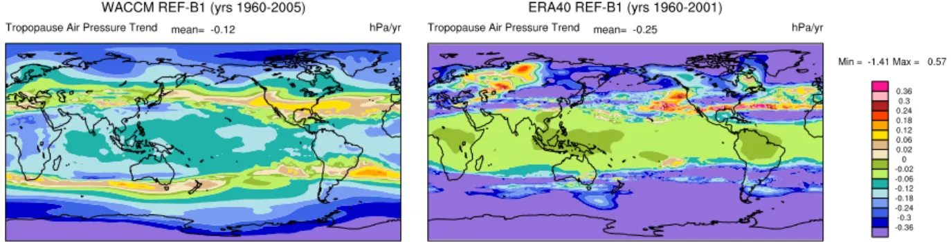
Finally, diagnostics can be fairly complex and methods combined. As an example, we show in Fig. 6 a map (using the “surfcontrend” routine) of the trends in lapse rate tropopause pressure at each point from a CCM (WACCM) and ERA40 reanalysis temperatures for the historical period from 1960– 2001. Here the code first calculates the tropopause pressure from temperature data (following Reichler et al., 2003) at each latitude and longitude, and then calculates a trend at
each point. The trends are then plotted on a map. This shows how complex diagnostics can be used to layer on top of each other. The CCMVal-Diag tool can also easily plot differences between the models and a “reference” (such as the ERA40 re-analysis in Fig. 6), as necessary. Other routines can quantita-tively compare zonal mean trends, illustrating the flexibility of the tool with a standard set of plot types.
4.2 Repeatable diagnostics
A strong principle for the CCMVal-Diag tool is support-ing model development as well as quantifysupport-ing model im-provements, both for different versions of individual CCMs and for different generations of community-wide collections of models used in international assessments. Accordingly, the CCMVal-Diag tool has incorporated diagnostic plots to specifically evaluate processes important for stratospheric ozone. As a start, process-oriented diagnostics from Eyring et al. (2006) have been implemented into the structure so they can be repeated with different model versions. Table 2 lists the plot types. In principle these can be applied to any vari-able, but these plots are generally run with specific variables (noted in the table). The numbers refer to figure numbers in Eyring et al. (2006). Note that this also serves as an example of specifically documenting diagnostics for the tool.
Fig. 6. Map of lapse rate tropopause pressure trends (hPa yr−1) from WACCM CCM and ERA40 reanalysis temperatures.
Table 2.Repeating plot types from Eyring et al. (2006).
Number Short Name Variables Description
1 vertline T Line plot of vertical profile differences
2 windzero U zero wind line descent in pressure
4 linets T 1-D timeseries plot (like tsline)
5a vertval O3, CH4, H2O, HCl zonal mean profile plot
5b meridval O3, CH4, H2O, HCl zonal mean line plot
7 linemon T, H2O annual cycle line plot (like monline)
8 vertts H2O vertical profiles over time
9 vertamp H2O amplitude and phase lag in vertical
12 profilets Cly profile and timeseries line plots (2 panel)
14 surfann Column O3 contour plot of a 2-D zonal mean over month
15 tsclimo Column O3 combination of timeseries and climatology
gray (E39C) models. This improvement is also seen in the zonal mean at 50 hPa (Fig. 7c and d). These results are used extensively to compare CCMVal-1 and CCMVal-2 models in the SPARC report on the evaluation of chemistry-climate models (SPARC-CCMVal, 2010).
Figure 8 shows the inorganic chlorine (Cly) climatologi-cal mean verticlimatologi-cal profile (A, C) and the time series (B, D) of 11 CCMVal-1 models (lower panel) and 12 CCMVal-2 mod-els (upper panel) similar to Fig. 12 of Eyring et al. (2006). Clyis a strong indicator of chlorine-induced ozone loss, and the rise in Clyfrom 1980 to 2000 and subsequent decline are a key metric for understanding the ozone hole. Observations are specified as attribute of the specific plot type. This routine can easily be used for any other chemical variable. Observa-tions of Clyare derived from HALOE HCl measurements in 1992 and Aura MLS HCl in 2005 as described by Eyring et al. (2006).
4.3 Quantitative metrics
Finally, the diagnostics and code can be used to develop quantitative grades for model performance. Quantitative per-formance evaluation is highly dependent on the choice of di-agnostics used. Here we merely show an example of how the CCMVal-diag tool has been used to derive several such
metrics. Following Waugh and Eyring (2008) and Gettelman et al. (2010), we show quantitative metrics for CCMVal-2 models in the upper troposphere and lower stratosphere (UTLS) in Fig. 9. These quantitative metrics compare model climatological means to different observations of winds, tem-peratures and trace species (see Gettelman et al., 2010 for details). The figure is derived from Fig. 7.39 of SPARC-CCMVal (2010). In this figure, grades from 0 to 1.0 were produced by the diagnostics tool by comparing model output to observations, and the results gathered into Fig. 9. Grades for the multi-model mean (MMM) are also calculated by the tool. The darker the color in Fig. 9 is, the better the model score. Variations on the overall bias metrics in Fig. 9 can also be easily added. These include statistical tests like root-mean-square (RMS) differences and “Taylor” diagrams of normalized errors and correlations.
5 Summary and future plans
A) CCMVal-1 H2O Equator MAR B) CCMVal-2 H2O Equator MAR
C) CCMVal-1 H2O 50 hPa MAR D) CCMVal-2 H2O 50 hPa MAR
Fig. 7. Comparison of March water vapor concentration simulated for the 1990s by models from CCMVal-2(B, D)and CCMVal-1 (A, C)
for equatorial water vapor profiles(A, B)and zonal mean 50 hPa(C, D). HALOE observations are shown as black dots, and the gray shading
is one standard deviation. Individual model colors and line-styles follow Figure 4.
versions of a model) against observations. It can also be used to evaluate the output from multiple models against ob-servations and/or against each other, e.g. chemistry-climate models (CCM) participating in the CCM Validation (CCM-Val) activity and climate models participating in the Coupled Model Intercomparison Project (CMIP).
The tool has the following features:
– Open Source
– Converts model output to standard format
– Analyzes and plots output
– Works on multi-model or single-model ensembles
– Integrates observations in multiple ways
– Flexible and Extensible
The tool has been used in several papers (Gettelman et al., 2010; Eyring et al., 2010a,b; Cionni et al., 2011), and has supported some of the analysis of SPARC-CCMVal (2010) and the World Meteorological Organization (2010) scientific
assessment of ozone depletion. It will operate on standard CF compliant NetCDF model output, the standard format used by CCMVal and CMIP.
The diagnostic code could easily be extended to cover Earth system models (ESMs). In principle, any 2-D (surface, zonal mean) or 3-D field can be processed and plotted, re-gardless of grid (whether land surface, ocean, etc), global or regional. Additional observations for the existing diagnostics or for new diagnostics can be easily implemented, allowing a comparison to multiple measurements if available. The code thus allows further extensions by different users for different applications and types of ESMs. These applications could, for example, include the verification of decadal climate pre-dictions, and the evaluation of aerosols, land surface or ocean parameters. The code also principally works for limited area (e.g. regional climate) models.
A) CCMVal-2 Cly 80S NOV B) CCMVal-2 Cly 50 hPa 80S OCT
C) CCMVal-1 Cly 80S NOV D) CCMVal-1 Cly 50 hPa 80S OCT
Fig. 8. 80◦S ClyNovember profile(A, C)and October time series(B, D)for 11 CCMVal-1 models(C, D)and 12 CCMVal-2 models(A,
B).(A, C)Climatological mean vertical profiles (1990 to 1999) at 80S in November for Clyin ppbv.(B, D)Time series of October mean
Antarctic Clyat 80◦S from CCM model simulations. Estimates of Clyfrom HALOE HCl measurements in 1992 and Aura MLS HCl in 2005
are shown. Individual model colors and line-styles follow Fig. 4.
0. 0.1 0.2 0.3 0.4 0.5 0.6 0.7 0.8 0.9 1.
Grade
TCPT PTP O3 H2O
. 1
AMTRAC3
CAM3.5
CCSRNIES
CMAM
CNRM-ACM
E39CA EMAC GEOSCCM LMDZrepro
MRI
NiwaSOCOL
SOCOL ULAQ
UMETRAC
UMSLIMCAT UKCA-METO UKCA-UCAM
WACCM
MMM
H2O PROF CO NORM GRAD@200 SEAS CYC H2O SEAS CYC O3 LMS MASS U@200
T
ropical
Dia
gnostics
Extr
a
-tr
opical
Dia
gnostics
Fig. 9. Quantitative metrics summary from CCMVal-2 models as reported in SPARC-CCMVal (2010), Fig. 7.39. Metrics are produced by
the CCMVal diagnostic tool ranging from 0 to 1 for each model. These metrics represent key aspects of the model performance in the upper troposphere and lower stratosphere (UTLS) tropics (upper) and extra-tropics (lower). MMM indicates the multi-model mean. Diagnostics
are described in Gettelman et al. (2010) and SPARC-CCMVal (2010). They represent tropical water vapor (H2O), ozone (O3), tropopause
pressure (PTP) and tropopause temperature (TCPT). Extra-tropical diagnostics are 200 hPa zonal wind (U200), mass of the lowermost
stratosphere (LMS MASS), seasonal cycles of O3and H2O, the meridional gradient of 200 hPa wind (GRAD200), normalized CO gradients
use of a known plot type. Modifications and diagnostics can be added to the code repository so others can use them.
We encourage users to modify the code and submit di-agnostics and extensions back to the CCMVal-Diag tool archive. Those interested in using the code are referred to the links in Appendix A to obtain the code and further in-structions on how to get started.
Appendix A
Further information
More information on the standard and the data request to run this tool can be found at
– http://www.pa.op.dlr.de/CCMVal/DataRequests/ CCMVal-2 Datarequest FINAL.pdf
For general information on the CCMVal project, see
– http://www.pa.op.dlr.de/CCMVal/
This document and the diagnostic code, with latest bug fixes and updates, are available by link from
– http://www.pa.op.dlr.de/CCMVal/CCMVal DiagnosticTool.html
Acknowledgements. The development of the CCMVal diagnostic tool was supported by the Atmospheric Chemistry Modeling and Analysis Program (ACMAP) grant NNX08AK54G and by the InfraStructure for the European Network for Earth System Modeling (IS-ENES) project (WP9/JRA3) which is funded by the European Commission under the 7th Framework Programme. Sup-port has also been provided by the National Center for Atmospheric Research (NCAR, USA), the Deutsches Zentrum f¨ur Luft- und Raumfahrt (DLR, Germany), the University of Toronto (Canada) and the National Institute for Water and Atmosphere (NIWA, New Zealand). We thank G. Bodeker and the entire staff of Bodeker Scientific for their assistance in planning and developing the tool. We thank S. Tilmes and K.-D. Gottschaldt for comments on this manuscript. NCAR is supported by the United States National Sci-ence Foundation. We acknowledge the modeling groups for making their simulations available for this analysis, the Chemistry-Climate Model Validation (CCMVal) Activity for WCRP’s (World Climate Research Programme) SPARC (Stratospheric Processes and their Role in Climate) project for organizing and coordinating the model data analysis activity, and the British Atmospheric Data Center (BADC) for collecting and archiving the CCMVal model output.
Edited by: A. Stenke
References
Brasseur, G. P. and Roeckner, E.: Impact of improved air quality on the future evolution of climate, Geophys. Res. Lett., 32, L23704, doi:10.1029/2005GL023902, 2005.
Cionni, I., Eyring, V., Lamarque, J. F., Randel, W. J., Stevenson, D. S., Wu, F., Bodeker, G. E., Shepherd, T. G., Shindell, D. T., and Waugh, D. W.: Ozone database in support of CMIP5 simulations: results and corresponding radiative forcing, Atmos. Chem. Phys., 11, 11267–11292, doi:10.5194/acp-11-11267-2011, 2011. Eyring, V., Butchart, N., Waugh, D. W., Akiyoshi, H., Austin, J.,
Bekki, S., Bodeker, G. E., Boville, B. A., Br¨uhl, C., Chipper-field, M. P., Cordero, E., Dameris, M., Deushi, M., Fioletov, V. E., Frith, S. M., Garcia, R. R., Gettelman, A., Giorgetta, M. A., Grewe, V., Jourdain, L., Kinnison, D. E., Mancini, E., Manzini, E., Marchand, M., Marsh, D. R., Nagashima, T., Newman, P. A., Nielsen, J. E., Pawson, S., Pitari, G., Plummer, D. A., Rozanov, E., Schraner, M., Shepherd, T. G., Shibata, K., Stolarski, R. S., Struthers, H., Tian, W., and Yoshiki, M.: Assessment of tem-perature, trace species, and ozone in chemistry-climate model simulations of the recent past, J. Geophys. Res., 111, D22308, doi:10.1029/2006JD007327, 2006.
Eyring, V., Chipperfield, M. P., Giorgetta, M. A., Kinnison, D. E., Manzini, E., Matthes, K., Newman, P. A., Pawson, S., Shepherd, T. G., and Waugh, D. W.: Overview of the New CCMVal Refer-ence and Sensitivity Simulations in Support of Upcoming Ozone and Climate Assessments and the Planned SPARC CCMVal As-sessment, SPARC Newsletter, 20–26, 2008.
Eyring, V., Cionni, I., Lamarque, J. F., Akiyoshi, H., Bodeker, G. E., Charlton–Perez, A. J., Frith, S. M., Gettelman, A., Kinni-son, D. E., Nakamura, T., Oman, L. D., PawKinni-son, S., and Ya-mashita, Y.: Sensitivity of 21st century stratospheric ozone to greenhouse gas scenarios, Geophys. Res. Lett., 37, L16807, doi:10.1029/2010GL044443, 2010a.
Eyring, V., Cionni, I., Bodeker, G. E., Charlton-Perez, A. J., Kinni-son, D. E., Scinocca, J. F., Waugh, D. W., Akiyoshi, H., Bekki, S., Chipperfield, M. P., Dameris, M., Dhomse, S., Frith, S. M., Garny, H., Gettelman, A., Kubin, A., Langematz, U., Mancini, E., Marchand, M., Nakamura, T., Oman, L. D., Pawson, S., Pitari, G., Plummer, D. A., Rozanov, E., Shepherd, T. G., Shibata, K., Tian, W., Braesicke, P., Hardiman, S. C., Lamarque, J. F., Mor-genstern, O., Pyle, J. A., Smale, D., and Yamashita, Y.: Multi-model assessment of stratospheric ozone return dates and ozone recovery in CCMVal-2 models, Atmos. Chem. Phys., 10, 9451– 9472, doi:10.5194/acp-10-9451-2010, 2010b.
Gettelman, A., Hegglin, M. I., Son, S.-W., Kim, J., Fujiwara, M., Birner, T., Kremser, S., Rex, M., A˜nel, J. A., Akiyoshi, H., Austin, J., Bekki, S., Braesike, P., Br¨uhl, C., Butchart, N., Chip-perfield, M., Dameris, M., Dhomse, S., Garny, H., Hardiman, S. C., J¨ockel, P., Kinnison, D. E., Lamarque, J. F., Mancini, E., Marchand, M., Michou, M., Morgenstern, O., Pawson, S., Pitari, G., Plummer, D., Pyle, J. A., Rozanov, E., Scinocca, J., Shepherd, T. G., Shibata, K., Smale, D., Teyss´edre, H., and Tian, W.: Multi-model assessment of the Upper Troposphere and Lower Strato-sphere: Tropics and Trends, J. Geophys. Res., 115, D00M08, doi:10.1029/2009JD013638, 2010.
Meehl, G. A., Covey, C., Taylor, K. E., Delworth, T., Stouffer, R. J., Latif, M., McAvaney, B., and Mitchell, J. F. B.: The WCRP CMIP3 Multimodel Dataset: A New Era in Climate Change Research, Bull. Am. Meteorol. Soc., 88, 1383–1394, doi:10.1175/BAMS-88-9-1383, 2007.
Morgenstern, O., Giorgetta, M. A., Shibata, K., Eyring, V., Waugh, D. W., Shepherd, T. G., Akiyoshi, H., Austin, J., Baumgaertner, A. J. G., Bekki, S., Braesicke, P., Br¸hl, C., Chipperfield, M. P., Cugnet, D., Dameris, M., Dhomse, S., Frith, S. M., Garny, H., Gettelman, A., Hardiman, S. C., Hegglin, M. I., J¨ockel, P., Kinni-son, D. E., Lamarque, J.-F., Mancini, E., Manzini, E., Marchand, M., Michou, M., Nakamura, T., Nielsen, J. E., Olivi´e, D., Pitari, G., Plummer, D. A., Rozanov, E., Scinocca, J. F., Smale, D., Teyss´edre, H., Toohey, M., Tian, W., and Yamashita, Y.: Review of the formulation of present-generation stratospheric chemistry-climate models and associated external forcings, J. Geophys. Res., 115, D00M02, doi:10.1029/2009JD013728, 2010. Reichler, T., Dameris, M., and Sausen, R.: Determination of the
Tropopause Height from gridded data, Geophys. Res. Lett., 30, 2042, doi:10.1029/2003GL018240, 2003.
SPARC-CCMVal: SPARC Report on the Evaluation of Chemistry-Climate Models, SPARC Report 5, WCRP-132, WMO/TD-1526, Stratospheric Processes and Their Role In Climate, World Meteorological Organization, 2010.
Taylor, K. E., Stouffer, R. J., and Meehl, G. A.: An Overview of CMIP5 and the Experimental Design, in press, Bull. Amer. Met. Soc, 93, 485–498, doi:10.1175/BAMS-D-11-00094.1, 2012. Uppala, S., Kallberg, P., Simmons, A., Andrae, U., da Costa
Bech-told, V., Fiorino, M., Gibson, J., Haseler, J., Hernandez, A., Kelly, G., Li, X., Onogi, K., Saarinen, S., Sokka, N., Allan, R., Ander-sson, E., Arpe, K., Balmaseda, M., Beljaars, A., van de Berg, L., Bidlot, J., Bormann, N., Caires, S., Chevallier, F., Dethof, A., Dragosavac, M., Fisher, M., Fuentes, M., Hagemann, S., Holm, E., Hoskins, B., Isaksen, L., Janssen, P., Jenne, R., McNally, A., Mahfouf, J.-F., Morcrette, J.-J., Rayner, N., Saunders, R., Simon, P., Sterl, A., Trenberth, K., Untch, A., Vasiljevic, D., Viterbo, P., and Woollen, J.: The ERA-40 re-analysis, Q. J. R. Meteorol. Soc., 131, 2961–3012, 2005.
Waugh, D. W. and Eyring, V.: Quantitative performance met-rics for stratospheric-resolving chemistry-climate models, At-mos. Chem. Phys., 8, 5699–5713, doi:10.5194/acp-8-5699-2008, 2008.