THE PORTUGUESE ENVIRONMENT, MACROEOCONOMIC SCENARIOS AND THE ESTIMATION OF LOSSES FOR CORPORATE SECTORS

(1)

A Work Project, presented as part of the requirements for the Awards of a Masters Degree in Finance from the NOVA – School of Business and Economics.

CREDIT RISK STRESS TESTING

THE PORTUGUESE ENVIRONMENT, MACROEOCONOMIC

SCENARIOS AND THE ESTIMATION OF LOSSES FOR

CORPORATE SECTORS

MARIA INÊS CUNHA MARTINS BATALIM #490

A Project carried out on the Financial Markets major, under the supervision of: Professor Samuel da Rocha Lopes

(2)

CREDIT RISK STRESS TESTING

THE PORTUGUESE ENVIRONMENT, MACROEOCONOMIC SCENARIOS AND THE ESTIMATION OF LOSSES FOR CORPORATE SECTORS

Acknowledgements

I would like to take the opportunity to express my deepest gratitude to my supervisor, Professor Samuel da Rocha Lopes, for his expertise, understanding and patience, which were fundamental to my work. I would also like to extend my appreciation to Professor Paulo Rodrigues for taking the time to help me. Finally, I cannot help to mention my family and friends for their care and support throughout this time.

Abstract

This study focuses on the development of a macroeconomic credit risk model for the prediction of corporate default rates, conditional on the observed economic environment. Data relative to the Portuguese economy was utilized for the development of the model, regarding the period from 2002 to 2012. The results suggest a clear link between macroeconomic factors, such as GDP, interest rates, unemployment and corporate indebtness, to the default rates observed. Furthermore, the introduction of a Merton-based analysis of the loss distributions permitted the analysis of expected and unexpected losses, alongside Basel II capital requirement evolutions.

(3)

1 Introduction

Recent years have seen great development in the credit risk (CR) area, being it is one of the greatest risk faced by banks nowadays, a fact which the current financial crisis greatly underlined. Therefore, it is of the utmost importance to study and understand CR, so as to model it in a way allowing financial supervisors, corporate and banking sectors to better define goals in dealing with the risk arising from credit portfolios. This work will develop a basis framework for CR modelling, which attempts, on the one hand, at determining default rates (DR), at an aggregate level, for six different sectors of corporates; whilst, on the other hand, at combining the obtained defaults with a multi-factor Merton-type multi-factor approach, which allows a richer analysis of loss distributions (LD)1 and correlation effects amongst the different sectors, known as sector concentrations.

This model will allow for the development of stress tests, which are indispensable measures for the risk control of a firm, as they provide not only a forward-looking analysis on CR, but also an analysis on their risk tolerance and the effectiveness of risk contingency plans. The stress scenarios developed will be mainly structural, focusing on creating specific states of the economy.

The work is organized as follows: Section 2 reviews the literature on the subject, whilst Section 3 provides a thorough description of the methodology in the macroeconomic model. Section 4 specifies the data utilized and the empirical model obtained. Sections 5 and 6 simulate the default rates and loss distributions. Stress testing analysis is developed in Section 7, and final remarks can then be found in Section 8.

(5)

2 Literature Review

Wilson (1997a, 1997b) developed the Credit Portfolio View2, one of the first models to

postulate an exogenous contemporaneous relationship between macroeconomic

variables and DRs. It has been studied and applied in the Austrian economy (Boss,

2002) – finding evidence on the link between industrial production, inflation, the stock

market, nominal interest rate and oil price and aggregate DR – and in the Finnish

economy (Virolainen, 2004) – using the same macroeconomic factors to study different

sectors of the economy, concluding that overall GDP deviations from trend, interest

rates and debt of a sector are significant in the analysis.

Several other studies have more recently focused on the macroeconomic determinants

of non-performing loans (NPLs). Salas and Saurina (2002) determine a great impact of

GDP growth on NPLs, finding evidence of rapid transmission between the

macroeconomic scenario and NPLs. Louzis et al. (2012) use a dynamic model to

determine NPLs sensitivity to GDP growth, lending rates, unemployment and public

debt, paired with bank-specific variables, finding strong evidence of a link between

these variables and DRs in the Greek banking sector.

In what concerns the design of LDs for specific portfolios, Bonti et al. (2006) build a

multi-factor portfolio model, which takes into account the correlation between

systematic risk factors – in that case sector correlations – present in the economy, when

determining losses in a certain portfolio. This model has been adapted and used to test

the German economy’s sensitivity to crisis in the automobile sector by Duellmann and

Erdelmeier (2009), finding evidence of significant increase in expected and unexpected

losses due to the effects of intersector correlations.

(6)

The literature on the subject of CR is vast and ever growing. Many authors underline

the importance of macroeconomic developments in the evolution of CR, still, recent

studies have shown that correlation between sectors has great impact in tail

measurements in CR. The model developed will attempt at combining these models, to

create a model that will not only be conditional on the state of the economy, but that

will also take into account the sector concentrations present in the specific portfolios.

3 Methodology – The Merged model

According to Simons and Rolwes (2008), the model developed should be classified as

fundamental, macroeconomic based and exogenous, since it assumes a maintaining

relationship between the economy and the macroeconomic factors used to model it.

This macroeconomic credit default model is characterized by the assumption of a

contemporaneous relationship between DR and a number of macroeconomic factors,

which depict a state of the economy at a specific point in time. Furthermore, it provides

a sectorial division of the economy which allows a deeper analysis of the effect of

similar macroeconomic variables in different sides of the economy, but allow also to

better grasp the effects each sector plays in the evolution of overall DRs. The work is

largely derivative of the model employed by Virolainen (2004), though it has been

complemented with the loss analysis from the Bonti et al. (2006), which allows an

extension to the analysis of sector concentration effects in LDs.

First and foremost, DRs must be set. These are defined in such a way that they will

depend on a macroeconomic index through a logistic functional form3:

!!,! = !

!!_!"#_!₍_! !,!)

(1)

(7)

where !!,! represents a specific DR for a sector at a given time and !_!,! the corresponding macroeconomic index for said industry at such time. As so, the

relationship between DR and the macroeconomic index will be such that the

macroeconomic index is positively correlated to the state of the economy and negatively

correlated to the DR, !!,!. The macroeconomic index can be defined as a logit

transformation of the DR of a specific sector at a given time,

!_!,! =L(!_!,!)=ln! !!!_!,!

!_!,!

(2)

The macroeconomic index will then be modelled on a set of macroeconomic variables,

!!,! =!!,!+!!,_!!_!,!+!!,_!!_!,!+!!,!!!,!+!!,! (3)

where !_!,! represents the vector coefficient for the i th

macroeconomic variable, !_!_,_!4_{, in}

the jth sector of the economy and !_!_,_!_{the error term of the regression, assumed}

independent and identically normally distributed.

Each of the explanatory macroeconomic variables will be expected to follow an

autoregressive process of order 25,

!_!,_!₌ !_!_,_! +!_!_,

!!!,!+!!,_!!_!,!+!!,!!!,!+!_!,! (4) where !_!_{a set of regression coefficients for each of the macroeconomic variables, and}

!_!_,_!_{the error term of the regression, independent and identically normally distributed.}

Using both equations (3) and (4) alongside the error terms6, it is possible to determine a

forecast on the evolution of each industry’s DRs and the corresponding macroeconomic

variables for a desired period, conditional on the observable state of the economy at the

end of the sample period.

4_{Independent variables will be described in further detail in the next section.}

5_{Following the model stated by Virolainen (2004).}

6_{Both the vector of error terms (}

!) and the variance-covariance matrix (Σ), defined as:

(8)

It is also possible to devise several different stress scenarios, resulting from changes in

the macroeconomic setting in each time set. Any of the macroeconomic variables can be

stressed, by introducing the specific shock into the simulated vector of error terms,

divided by its standard deviation, which will allow the normalization of the vector. By

maintaining other variables stable, it will be possible to evaluate specific shocks in the

economic environment, and determine the response of DRs to those changes.

Finally, after forecasted DRs have been determined, it is possible to use a multi-factor

portfolio model7, with a specific predetermined representative portfolio of the

Portuguese banking system, to determine LDs for the different scenarios created8.

Crucial to this model is the idea that a certain loan will default if the default trigger _!!

falls bellow the default barrier !_!9_{. Said trigger is defined by two risk components:}

!! = !.!_!₍!₎+ 1−!!.!! (5)

The first is the sector dependent systematic risk factor _!_! ! and the second is the

borrower dependent or idiosyncratic risk factor !_!_{, which are weighted according to}

asset correlation, determined by the Basel II formula for corporates10. Both,

!!! !!"#!!!, are pairwise independent and present a joint standard normal distribution.

The systematic risk factor !! ! will be dependent on the correlation between DRs in

different sectors and a number of independent standard normal risk factors !!,!

!! ! = !! ! ,!

!

!_!! .!!

11

(6)

7_{Developed by Bonti et al. (2006) and further developed by Duellmann and Erdelmeier(2009).}

8_{This model will replace the binomial draw used by Virolainen (2004) to determine loss distributions.}

9

Where !_!_{will be the inverse of the cumulative normal distribution for the specific loan’s DR.} 10_!""#$

!!"#_r!"#$%&'_!₍_r₎₌0_.₁₂_×!!!!

!"_×_!"

!!!!!" +0.24×

!!!!!"×!" !!!!!"

11_The_!

(9)

Finally, through the use of a Monte Carlo simulation, it is possible to determine the

losses of a specific portfolio, which will allow the analysis of the average loss an

institution is expected to have in a certain year – through expected losses12, a function

of DR, exposure-at-default and loss-given default13 – but also the analysis of possible,

yet unforeseen losses – unexpected losses14. Furthermore, the analysis of capital

requirements’15 evolution will, alongside the previous measures, be crucial to what Sir

David Walker (2009) considers essential in the context of stress testing, “to understand

the circumstances under which the entity would fail and be satisfied with the level of

risk mitigation that is built in”.

4 Data and Default modelling

The afore-described model will be adapted to the Portuguese reality and data. Since data

on DRs is not readily available for the general public, we take a broader definition of

default and employ quarterly data on non-performing loans from non-financial firms16,

available for the period from the 4th quarter of 2002 until the 2nd quarter of 2012,

obtainable through the Bank of Portugal.

This set of data is then separated into 6 different sectors17, according to the NACE 2

sections18, which are: agriculture (AGR); industry and manufacturing (I&M);

construction and real estate (CRE); trade, hotels and restaurants (THR); support

12_!"#$%&$'

!!"##$#₌_!"._!"#_.!"#

13_{Loss given default (LGD) is assumed constant at a 45% level, slightly less conservative than the usual}

rule-of-thumb of 50% recovery rate. 14

Unexpected losses represent the difference between Value-at-Risk at a certain confidence level, usually 99% or 99.9%, and the expected losses in a portfolio.

15_{Capital requirements are calculated using the Basel II formula:}

!= !"#_._Φ ₁₋_! !!,!

.Φ!! !" + ! 1−!

!,!

.Φ(0_.999₎ ₋_!".!"# _. ₁₋_1.5_×!₍_!"₎!!_. ₁ + _!₋_2.5 _.!₍_!"₎

16

The ratio of non-performing loans will from now only commonly be referred to as default rate.

17_{Statistical information obtained on non-performing loans ratio was broken down into all 21 NACE 2}

sections. Using yearly information on the average number of firms per section it was possible to group these ratios into 6 different sectors of the economy.

(10)

activities (SA); and other services and activities (OSA). Assuming the data on

non-performing loans could be considered a close proxy to DRs in the corporate sector,

using data on total number of companies, sector DRs were compiled. Figures 2.1 and

2.2, in Section 2 of the Appendix, show the evolution of the DRs for the period under

consideration, from 2002:Q4 to 2012:Q2, a set of 42 observations.

As can be seen, sector DRs appear highly correlated, following a downward trend

approximately until 2008, from which on there is an increase in all sectors, a behaviour

most certainly arising from the global financial crisis, a moment of economic downturn

which affected all sectors of the economy. This analysis shows a greater impact in the

CRE sector, a result of the construction boom experienced in the previous years due to

what could be considered a real-estate bubble. Sectors 2 and 4, I&M and THR, follow

CRE as the most affected sectors by the economic downturn. On the other hand, though

also showing signs of increase, the remaining sectors display smoother paths.

This can be analysed in Figure 2.2, which depicts the evolution of the overall DR in the

economy. The lowest value taken by the overall DR is of 1.80% in the last quarter of

2007, from which on there is a clear upward trend, up to the maximum value of 7.90%

in the second quarter of 2012, confirming the effect of the 2008 financial crisis and

further on of the sovereign debt crisis affecting the Euro Zone.

The calculated sectorial DRs will suffer a logit transformation, creating the dependent

variable, the sectorial macroeconomic index. Following previous work on the subject,

the main factors aiming at explaining DRs are based on three different sets of measures:

profitability, indebtedness and interest rates. Defining the model as such will allow a

parsimonious analysis, focusing on factors which, whilst extremely significant to the

(11)

the effects their variations take on the evolution of DRs and LDs. Furthermore, the same

variables are used to explain DRs across sectors, permitting an analysis of the effects of

macroeconomic indicators separately yet transversely through sectors.

For profitability, GDP is used, both the annual percentage growth rate and a measure of

deviations from trend, which are the residuals obtained by regressing log GDP on a time

trend. As an additional measure, unemployment rate is also utilized. As for

indebtedness, an index is created19 which presents the total debt of the sector divided by

the value added by said sector. This index, though specific for each sector, does not

undermine one of the main characteristics of the model, which is its similarity across

sectors. Finally, for interest rate measures, variables included are the Euribor – 3-month,

6-month and 12-month – but also the spread between the average interest rate charged

on non-financial firms and the Euribor, also at three different maturities.

Taking into account that the dependent variable will be the macroeconomic index, GDP

measures will be expected to carry a positive sign, since a higher GDP implies a better

state of the economy, a higher macroeconomic index, and in turn a lower DR. On the

other hand, unemployment is expected to carry a negative sign, as will interest rate

variables and the debt index20.

The modelling is done through the use of the seemingly unrelated regressions (SUR)

model, which assumes the dependent variables of different equations are in fact

correlated21. The use of the SUR model allows an increase in the efficiency of the

estimators, since it takes into account the contemporaneous correlations between the

19

Debt index is based on the work of Virolainen (2004).

20_{Virolainen (2004) postulates a negative relationship between debt ratio and the macroeconomic index,}

although other studies (Pesola, 2001; Kalira and Scheicher, 2002) have found these results to be ambiguous.

(12)

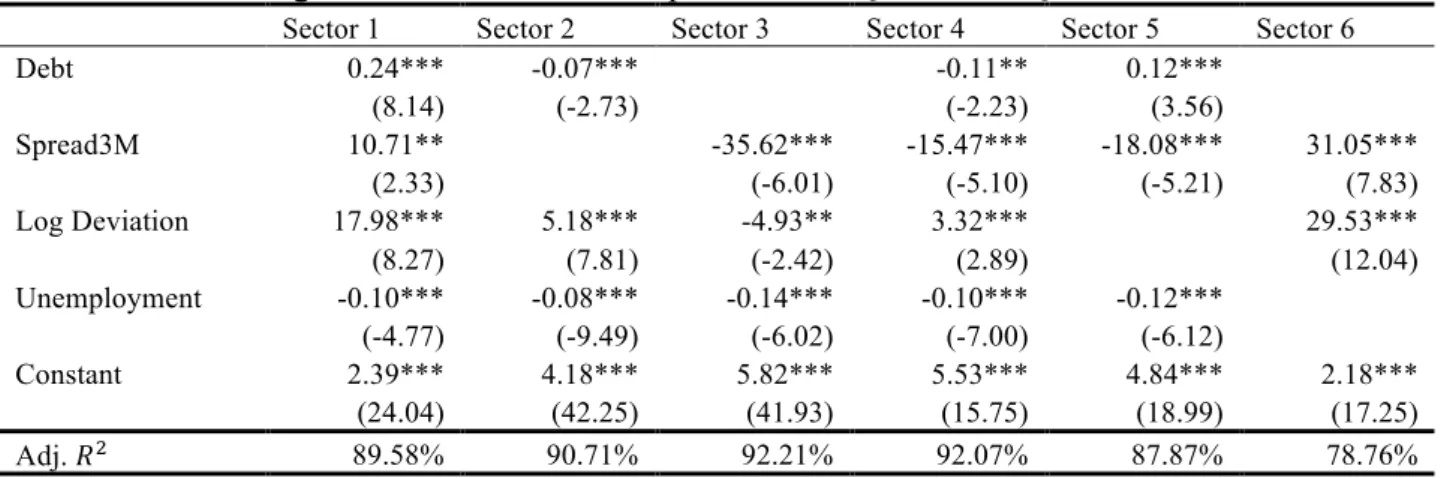
error terms of different regressions, transforming them into zero. The results of the SUR

estimates are reproduced in Table 3.2, Section 3 in the Appendix. The final independent

variables used are: the sectorial debt index; the 3-month spread, which proved far more

significant than the Euribor, since it displays a far smaller correlation with the GDP

variable; the deviations from GDP trend, since the growth rate does not fully attain the

impact of GDP changes in the dependent variable, and finally, the unemployment rate22.

In general, the Adjusted !!measure suggests the model is well specified and has a quite

high explanatory power, averaging 90% across all sectors. Nevertheless, some issues

must be referred, regarding both the sign carried by some of the explanatory variables

and also their statistical significance.

First and foremost, debt index, though significant in most sectors, proved to be

statistically not significant at a 10% level both for CRE sector and for OSA.

Furthermore, though being significant at a 1% significance level, for sectors 1 and 5,

AGR and SA respectively, it carries a positive sign, unlike what was expected. It may

be realistic to justify this on the specific characteristics of the Portuguese universe of

non-financial firms. According to the Portuguese Central Bank Balance-Sheet Database,

in 2009, the large majority of the industrial fabric in Portugal was composed of small

and medium companies. Firms of this size are usually bank-dependent and have access

only to short-term loans, especially when considering a large part of the sample period

is affected by the financial crisis, which exponentially increased banks’ risk aversion,

therefore conditioning firms’ access to loans. The variable was, nonetheless, included in

the model, since it showed statistical relevance.

22

(13)

Other explanatory variables were introduced, including Production Index, the

Harmonized Index of Consumer Prices, and the returns on the PSI 20, but proved to be

generally statistically not significant, with next to no impact in the adjusted !! measure.

As for the autoregressive processes, they provided an adequate model for the evolution

of the explanatory variables – the results can be found in Table 3.3, Section 3.

5 Simulating Default Rates

Following the construction of the model and its application to the Portuguese data, it is

possible to determine a set of DRs for a period in the future through the use of equations

(1) and (4), as well as the error terms and their respective variance-covariance matrix.

The first step is to decompose the variance-covariance matrix using the Cholesky

decomposition method23. Secondly, a matrix of standard normal vectors of (!+!₎_×_1!

dimensions is drawn, _!!!!, which will be transformed into the vector of innovations

through !!!! = !′!!!!. This will provide simulated realisations of the error terms, that

together with the AR(2) processes will determine paths for the explanatory variables,

taking into account the correlations between macroeconomic factors.

Using equation (3) and its determined coefficients alongside equation (1), it is possible

to determine the simulated path, for a period of 12 quarters, for the sectorial DRs.

It is important to analyse what should be considered a baseline case, one in which there

are no shocks in the economy, therefore its state is determined solely by the equations

estimated for the development of the macroeconomic variables and the verified scenario

in the end of the sample. Figure 5.1, Appendix, demonstrates a clear, though not steep

for most of the sectors, upward trend. The analysis of the overall DR confirms the

23_{The Cholesky decomposition matrix is defined as C, so that}

(14)

expectations of further growth in DRs, despite no shocks to the economy. This is most

possibly a result of the sample collected, which includes a more than 4 year-wide

recessionary period, representing around 20% of the sample, thus creating a negative

bias in the analysis.

6 Loan Portfolio and Loss Distribution

The continuation of the analysis of the macroeconomic model developed requires the

construction of LDs associated with the forecasted DRs. For said purpose, data on a

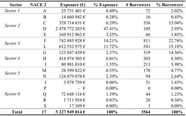
specific loan portfolio was procured. The portfolio is representative of the Portuguese

economy, constituted by 3564 borrowers, with a total exposure of 5.227.949.014€24_–

further detail on the portfolio can be found in Section 4, Appendix.

The next subsections will allow for a brief analysis of the LDs generated by the

aforementioned baseline _{scenario. The correlation matrix between sectors is assumed}

constant, which is one of the shortcomings of the analysis presented, although it is still

possible to analyse the short-term effects of the different scenarios.

Employing the DRs obtained from the baseline_{case, it was possible to reach the LD}

generated by the average of the next 4 quarters forecasted yearly default probabilities.

Due to the model’s biasedness towards a negative scenario in the future, results are

above what would be expected, with expected losses (EL) arising to 2.74% of the total

exposure, and unexpected losses (UL) of the 99% (99.9%) percentile of 6.55% (8.13%)

(see Table 5.1_{, Appendix), meaning that there is a 1%(0.1%) possibility there will be}

losses in the portfolio which will exceed those expected by 239% (279%).

24

(15)

The LD presents skewedness to the left, since the majority of the simulated losses are in

the [0,10] interval25. Lastly, the baseline _{scenario demands capital reaching 15.89% of}

the total risk-weighted assets, showing the clear signs of negative outlook predicted for

the Portuguese economy in the forecasted period.

7 Stress Tests

As aforementioned, the model developed allows for an analysis of specific shocks in the

economy. We will focus on the effects of negative shocks in GDP, increases in interest

rate spreads and finally a combination of both of these scenarios. Furthermore, it proved

relevant to scrutinise effects of persistent shocks, versus those of less lasting effects,

still with the same magnitude – shocks considered persistent last over 4 quarters, whilst

the other only 2. An analysis of the effects on DRs will first be achieved, followed by

an analysis of the LDs for the representative portfolio and, finally, an analysis of

sectorial capital requirements will be postulated. Probabilities of default utilized in the

LD reflect only the first year average; nevertheless, the effects on the DRs can be seen

throughout the 12 quarter forecasted period.

The analysis focuses on the stress testing of the macroeconomic variables. Yet, through

the use of the multi-factor model, it is also possible to stress other components of the

model which were, for purposes of simplicity, maintained constant, such as the

Loss-Given-Default – maintained at a constant 45% level – and the sector correlation matrix.

GDP Stress Scenarios

Four different scenarios of stress are analysed, two mild – representing deviation from

trend to increase 3% over a one-year period – and two extreme – demonstrating 6%

decreases, one being persistent and the other not.

(16)

The not persistent scenario takes an initial larger toll on the DRs, as would be expected

given the assumption of larger changes. However, towards the end of the period, both

scenarios converge, as can be seen in Figure 6.1, Appendix.26 DRs show increases

averaging 0.85%, for the mild scenario, whilst the extreme scenario shows jumps in

DRs nearing 2.20%.

Sector-wise analysis of DRs allows the conclusion that the SA sector shows the highest

response to GDP changes, exponentially growing by more than 120% by the end of the

12 quarters. It is followed closely by the CRE sector, which shows an average increase

of 107%. These results come to confirm the expectations that recent years’

developments in the Portuguese economy greatly affect the model – in the last 4 years,

the GDP downturn has been in line with the demise of several CRE sector firms, due to

the bursting of the real estate bubble, and has shown great impact in the service sector,

mostly comprised in the SA sector.

Both the AGR sector and the OSA sector show smaller responses, actually decreasing

over time in the mild scenario. When analysing the evolution of these sectors’ DRs over

the previous year, which have already comprised a significant GDP downturn, it is clear

that their paths have been far smoother than those of remaining sectors, fact taken into

account by the model generating the milder responses seen. Overall, DRs show jumps

of over 60% from the observed values in 2012:Q2.

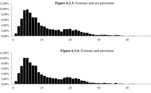
In what regards the LDs, seen in Figure 6.3, Appendix, increases in ELs around 0.38%

of the total exposure are observed, when compared to the baseline scenario, and ULs in

the 99% (99.9%) percentile show intensifications of 0.26% (0.81%) of the total

exposure. Finally, the rise in capital requirements is also moderate, increasing from the

(17)

observed 15.89% in the baseline scenario to an average of 16.26% in the mild scenario

and 16.64% in the extreme scenario27.

Interest Rate Stress Scenarios

Much like the previous analysis, there are four scenarios under scrutiny, two in which

the spread increase is of 1.5% and two where it is of 3%. Similarly, we see the effect of

not persistent shocks in the beginning of the forecast, but final results are nearly equal.

The sectorial analysis shows, yet again, Sectors 3 and 5 to have greater sensitivity to

changes in the interest rate, increasing by more than 150% from the values in 2012:Q2.

THR sector follows in a close third, jumping nearly 100%. In this case, the three sectors

mentioned present the largest debt ratios, proving the link between the average level of

debt level in an industry and its sensitivity to the interest rate level is present.

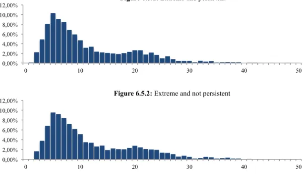
The LD analysis demonstrates that, despite the initial analysis of DRs indicating larger

variations in the DRs, overall the ELs are lower than those found in the GDP scenarios,

with increases from the baseline scenario averaging 0.16% of the total exposure. UL,

99% and 99.9%, show also little increase relative to the baseline scenario, respectively

0.03% and 0.10% of total exposure. Last but not least, capital requirements, which

depend directly on the DRs, show larger increases from the baseline, 0.96% in the

extreme case and 0.53% in the mild scenario.

Interest Rate and GDP Stress Scenario

In the final stress analysis, both the extreme scenarios of GDP and interest are

combined. As would be expected, Sectors 5 and 3 show the greatest responses to the

shock, although all sectors DRs increase by more than 15%.

(18)

ELs increase by 0.73% of total exposure, relative to the baseline_{scenario, and by 0.5%}

and 0.21% relative to the extreme_{interest scenarios and GDP scenarios, respectively.}

UL are also higher by 0.31% and 0.78% for 99% and 99.9% percentiles, respectively.

Overall, the LD presents fatter tails and a smaller bias towards the left when compared

to the baseline_{and other}extreme_scenarios.

This scenario does predict smaller losses than those that would arise simply from the

addition of losses in the individual stress cases. This result, though counter-intuitive,

arises from the fact that in previous analyses the correlation between macroeconomic

factors is taken into account. Therefore, changes in the spread variable – in the case of

the GDP stress scenarios – or the GDP variable – in the interest stress scenarios – are

already foreseen even in the case of only one macroeconomic variable being stressed.

8 Conclusions

This work provides an analysis of the merger of two models: one which allows the

forecasting of sector-wide DRs based on the current macroeconomic conditions and

their evolution, and another which takes into account inter-sector correlations and their

effect in the predicted losses for a specific portfolio. It provides a simple and

understandable analysis – both at an aggregate level but also through the use of a

representative portfolio of the Portuguese economy –, yet comprises the necessary tools

to allow for the construction of several stress scenarios, be it of macroeconomic

fluctuations or changes in the underlying hypothesis – as the recovery rate and the

correlation between sectors of the economy –, the analysis of which are crucial to the

understanding of default and loss evolutions.

Overall, the model showed to be adjusted to the current Portuguese macroeconomic

(19)

evolution of DRs across the economy. The indebtedness measure evidenced more

ambiguity in its results, most possibly determined by the overall characteristics of the

Portuguese corporate sector, characterized by small and medium sized firms, with lower

access to the debt markets and debt in general.

Nonetheless, some shortcomings must be taken into account, especially those arising

from data availability. The time span to which the data is referent, from 2002 to 2012,

includes several years of economic downturn, which lead to the display of a negative

bias in the general evolution of macroeconomic variables in the market, deeming the

baseline _{scenario analysis more adverse than initially expected. Still, analysis of}

different scenarios is possible, considering the strictness of the initial case is considered.

Further extensions can be made to the model. It would be interesting to allow for more

complex models to determine the forecasts of macroeconomic variables. Moreover, it

would be especially noteworthy to allow default rates to depend not only on the sector

of the economy to which they pertain, but also on the score associated with that specific

loan. Furthermore, a deeper analysis of the sector correlations in times of financial

distress would greatly improve the model, by allowing specific stress scenarios to be

adjusted according to the determined sector correlation associated with that specific

environment. Additionally, the model allows for the study of different portfolios,

allowing the analysis of specific credit portfolios pertaining to specific banks or firms.

All in all, the analysis conducted could be of great value to the Portuguese economy, be

it in the area of credit risk management, or even for financial supervisory purposes or

even financial stability analysis, proving the model to be a valuable tool in such times of

(20)

References

Bhimani, A , Gulamhussen, M and Lopes, S. 2009. “The effectiveness of auditor’s going-concern evaluation as an external governance mechanism: Evidence from loan defaults”. The International Journal of Accounting, 44(2009), 239-255.

Bhimani, A , Gulamhussen, M and Lopes, S. 2010. “Accounting and non-accounting determinants of default: An analysis of privately-held firms”. Journal of Accounting Public Policy, 29(2010), 517-532.

Bonti, G, Kalkbrener, M., Lotz, C. and Stahl, G. 2006. “Credit risk concentrations under stress.” Journal of Credit Risk, Volume 2, Number 3: 115-136.

Boss, M. 2002. “A Macroeconomic Credit Risk Model for Stress Testing the Austrian Credit Portfolio”. Financial Stability Report 4, Oesterreichische Nationalbank.

Boss, M., Fenz, G., Pann, J., Puhr, C., Schneider, M., and Ubl, E. 2009. “Modeling credit risk through the Austrian business cycle: An update of the OeNb model”. Financial Stability Report, 17, 85-101.

Duellmann, K. and Erdelmeier, M. 2009, September. “Crash Testing German Banks”.

International Journal of Central Banking, Volume 5, Number 3.

Kalirai, H. and Scheicher, M. 2002. “Macroeconomic stress testing: Preliminary Evidence for Austria”. Financial Stability Report3, Oesterreichische Nationalbank.

Louzis, P. & Vouldis, A. & Metaxas, V. 2012, April. “Macroeconomic and bank-specific determinants of non-performing loans in Greece: A comparative study of mortgage, business and consumer loan portfolios.” Journal of Banking and Finance, Volume 36, Issue 4.

Pesola, J. 2001. “The role of macroeconomic shocks in the banking crisis”. Bank of Finland Discussion Paper, No. 6/2001.

Salas, V. and Saurina, J. 2002. “Credit Risk in Two Institutional Regimes: Spanish Commercial and Savings Banks.” Journal of Financial Services Research, 22 (3): 203–24.

Simons, D. and Rolwes, F. (2009). “Macroeconomic default modelling and stress testing”.

International Journal of Central Banking, 5(3), 177-204.

Vlieghe, G. 2001. “Indicators of fragility in the UK corporate sector”. Bank of England

Working Paper, No. 146.

Virolainen, K.. 2004. “Macro testing with a macroeconomic credit risk for Finland”. Bank of Finland Discussion Paper, No. 18/2004.

Wilson, Thomas C. 1998, October. “Portfolio Credit Risk”. Federal Reserve Bank of New York Economic Policy Review.

Walker, D. 2009. “A review of corporate governance in UK banks and other financial industry entities”.

(21)

Appendix

Section 1: Sector division

For purposes of simplicity and comparability, sector division was made according to NACE 2 sections; the first level division of economic activities consisted of 21 alphabetical codes28, which were grouped into 6 sectors as follows:

Section 2: Evolution of DR – Aggregate and sectorial

28_{Four of the sections were not included in the analysis due to the nature of the activities: financial and}

insurance activities (K); public administration and defence; compulsory social security (O); Activities of households as employers; undifferentiated goods and services; producing activities of households for own use (T); and activities of extraterritorial bodies and organization (U).

Table 1.1:NACE 2 Sector Division

Number Sector NACE 2 Definition Section

1 Agriculture Agriculture, Forestry and Fishing A

2 Industry &

Manufacturing

Mining and quarrying Manufacturing

Electricity; Gas; Steam and air conditioning supply

Water Supply; Sewerage. Waste Management and Remediation activities

B C D E

3 Construction & Real

Estate

Construction Real estate activities

F L

4 Trade. Hotels and

Restaurants

Wholesale and retail trade; Repair of motor vehicles and motorcycles Accommodation and food services activities

Transportation and storage

G H I

5 Support activities Professional, scientific and technical activities

Administrative and support service activities

M N

6 Other services and

activities

Information and communication Education

Human health and social work activities Arts, entertainment and recreation Other services activities

J P Q R S 0,00% 5,00% 10,00% 15,00%

Figure 2.2: Evolution of sector default rates

Sector 1 Sector 2 Sector 3 Sector 4 Sector 5 Sector 6 0,00%

2,00% 4,00% 6,00%

(22)

Section 3: Empirical model

Table 3.1: Variable Definition

Variables Definition

Macroeconomic Index Logit transformation of each sector’s default rate

Debt Ratio between the total debt of a sector and the value added per said sector 3-Month Spread Spread between the yearly interest rate charged to NFC and the 3 month Euribor GDP Residuals of log real GDP regressed on a constant and a time trend

Unemployment Yearly rate of total unemployment

Table 3.2: SUR Regression estimates for the period 2002:Q4 to 2012:Q2

Sector 1 Sector 2 Sector 3 Sector 4 Sector 5 Sector 6

Debt 0.24*** -0.07*** -0.11** 0.12***

(8.14) (-2.73) (-2.23) (3.56)

Spread3M 10.71** -35.62*** -15.47*** -18.08*** 31.05***

(2.33) (-6.01) (-5.10) (-5.21) (7.83)

Log Deviation 17.98*** 5.18*** -4.93** 3.32*** 29.53***

(8.27) (7.81) (-2.42) (2.89) (12.04)

Unemployment -0.10*** -0.08*** -0.14*** -0.10*** -0.12*** (-4.77) (-9.49) (-6.02) (-7.00) (-6.12)

Constant 2.39*** 4.18*** 5.82*** 5.53*** 4.84*** 2.18***

(24.04) (42.25) (41.93) (15.75) (18.99) (17.25)

Adj. _!! _89.58% _90.71% _92.21% _92.07% _87.87% _78.76%

P-value: *- significant at a 10% level; **-significant at a 5% level; ***-significant at a 1% level 0

5 10

15 Figure 3.3: Debt index evolution

DEBT 1 DEBT 2 DEBT 3 DEBT 4 DEBT 5 DEBT 6 0,00%

1,00% 2,00% 3,00% 4,00% 5,00% 6,00% 7,00%

Figure 3.1: 3-Month Spread

-2,00% -1,00% 0,00% 1,00% 2,00%

(23)

Section 4: Loan Portfolio characteristics

Table 4.1:Loan Portfolio characteristics

Sector NACE 2 Exposure (€₎ _{% Exposure} _{# Borrowers} _{% Borrowers}

Sector 1 _A _{25 731 401}€ _0.49% ₇₂ _2.02%

Sector 2

B 14 660 942 € _0.28% ₁₆ _0.45% C 328 714 651 € _6.29% ₅₃₆ _15.04% D 2 478 772 283 € _47.41% ₁₀₅ _2.95% E 169 912 962 € _3.25% ₆₆ _1.85%

Sector 3 F 742 885 928 € 14.21% 811 22.76%

L 612 532 975 € _11.72% ₅₄₁ _15.18%

Sector 4

G 123 847 439 € _2.37% ₅₁₉ _14.56% H 418 974 305 € 8.01% 303 8.50% I 80 981 010 € 1.55% 213 5.98%

Sector 5 M 28 599 822 € 0.55% 170 4.77%

N 124 879 078 € _2.39% ₉₄ _2.64%

Sector 6

J 3 078 759 € _0.06% ₅₁ _1.43%

P - € _0.00% ₀ _0.00%

Q 72 648 116 € _1.39% ₄₄ _1.23% R 1 711 954 € _0.03% ₂₀ _0.56% S 17 389 € _0.00% ₃ _0.08%

Total 17 5 227 949 014 € _100% ₃₅₆₄ _100%

Section 5: Baseline Scenario

Table 3.3: Autoregressive process of order 2 for the period of 2002:Q4 to 2012:Q2

Debt 1 Debt 2 Debt 4 Debt 5 Spread3M LogDeviation Unemployment

L1 0.94*** 0.95*** 0.78*** 0.82*** 1.07*** 1.24*** 1.39*** (29.20) (5.41) (4.51) (4.85) (6.14) (7.61) (9.09)** L2 0.07 0.05 0.03 -0.04 -0.01 -0.31* -0.34 (-0.38) (0.26) (0.20) (-0.26) (-0.51) (-1.81) (-2.31) Constant 0.08 0.04 1.49* 1.69* 0.001 -0.001 -0.03 (0.61) (0.14) (1.78) (2.03) (0.58) (-0.63) (-0.14)

Adj. !! _98.70% _92.69% _62.65% _59.18% _85.66% _82.32% _97.77% P-value: *- significant at a 10% level; **-significant at a 5% level; ***-significant at a 1% level

Table 5.1:Loss analysis in the baseline _scenario

Baseline Expected Loss 2.74% Unexpected Loss (99%) 6.55% Unexpected Loss (99.9%) 8.13% Capital Requirements 15.89% 0,00% 5,00% 10,00% 15,00% 20,00% 25,00% 30,00% 35,00%

Figure 5.1: Default rates per sector in

baseline scenario

Sector 1 Sector 2 Sector 3

Sector 4 Sector 5 Sector 6

(24)

Section 6: Stress Tests

Table 6.1: Analysis of DRs in GDP rate stress tests

Extreme Mild

Persistent Not Persistent Persistent Not Persistent Persistent - Not Persistent -0.13% -0.05%

0.05%

Differences to Baseline 2.13% 2.26% 0.76% 0.93%

Extreme - Mild 1.24% 1.32% – –

Table 6.2: Analysis of DRs in Interest rate stress tests

Persistent Not Persistent Persistent Not Persistent Persistent - Not Persistent -0.11%

0.11%

-0.08% 0.08%

Differences to Baseline 2.91% 2.79% 1.07% 1.33%

Extreme - Mild 1.54% 1.57% – –

7,50% 9,50% 11,50% 13,50% 15,50% 17,50%

Figure 6.2: Analysis of Interest rate stress test scenarios overall DR

Extreme Persistent Extreme Not Persistent Mild Persistent Mild Not Persistent 7,50% 8,50% 9,50% 10,50% 11,50% 12,50% 13,50% 14,50% 15,50%

Figure 6.1: Analysis of GDP stress test scenarios overall DR

Extreme Persistent Extreme Not Persistent Mild Persistent Mild Not Persistent

7,50% 9,50% 11,50% 13,50% 15,50% 17,50%

Figure 6.3: Analysis of GDP and Interest rate stress test scenarios overall

DR

Extreme Persistent Extreme Not Persistent 0,00% 2,00% 4,00% 6,00% 8,00% 10,00% 12,00%

0 10 20 30 40

F

re

q

u

en

cy (% of s

imu lati os n ) Loss Class

(25)

Table 6.3: Analysis of DRs in GDP and Interest rate stress tests

Extreme

Persistent Not Persistent Persistent vs. Not Persistent -0.13%

0.13%

Differences to Baseline 2.13% 2.26%

Table 6.4: Loss distribution analysis of GDP stress tests

Persistent Not Persistent Persistent Not Persistent

Expected Loss 3.31% 3.20% 2.95% 3.01%

Unexpected Loss (99%) 7.01% 6.84% 6.64% 6.73%

Unexpected Loss (99.9%) 8.83% 8.94% 9.02% 8.96% Capital Requirements 16.55% 16.72% 16.22% 16.30%

Table 6.5: Loss distribution analysis of Interest Rate and GDP stress tests

!! Extreme

!! Persistent Not Persistent

Expected Loss 3.55% 3.38%

Unexpected Loss (99%) 6.87% 6.86%

Unexpected Loss (99.9%) 8.93% 8.91%

Capital Requirements 17.61% 17.87%

Figure 6.3: Loss distributions of GDP stress tests

0,00% 2,00% 4,00% 6,00% 8,00% 10,00% 12,00%

0 10 20 30 40

Figure 6.3.1: Mild and not persistent

Table 6.5: Loss distribution analysis of Interest Rate stress tests

!

Persistent Not Persistent Persistent Not Persistent

Expected Loss 2.95% 2.99% 2.82% 2.85%

Unexpected Loss (99%) 6.64% 6.60% 6.54% 6.54%

Unexpected Loss (99.9%) 8.29% 8.30% 8.18% 8.15% Capital Requirements 16.40% 16.45% 16.16% 16.23%

0,00% 2,00% 4,00% 6,00% 8,00% 10,00% 12,00%

(26)

Figure 6.4: Loss distributions of Interest Rate stress tests 0,00%

2,00% 4,00% 6,00% 8,00% 10,00% 12,00%

0 10 20 30 40

Figure 6.3.3: Extreme and not persistent

0,00% 2,00% 4,00% 6,00% 8,00% 10,00% 12,00%

0 10 20 30 40

Figure 6.3.4: Extreme and persistent

0,00% 2,00% 4,00% 6,00% 8,00% 10,00% 12,00%

0 10 20 30 40

Figure 6.4.1: Mild and not persistent

0,00% 2,00% 4,00% 6,00% 8,00% 10,00% 12,00%

0 10 20 30 40

Figure 6.4.2: Mild and persistent

0,00% 2,00% 4,00% 6,00% 8,00% 10,00% 12,00%

0 10 20 30 40

(27)

Figure 6.5: Loss distributions of Interest Rate and GDP stress tests

0,00% 2,00% 4,00% 6,00% 8,00% 10,00% 12,00%

0 10 20 30 40

Figure 6.4.4: Extreme and persistent

0,00% 2,00% 4,00% 6,00% 8,00% 10,00% 12,00%

0 10 20 30 40 50

Figure 6.5.2: Extreme and not persistent

0,00% 2,00% 4,00% 6,00% 8,00% 10,00% 12,00%

0 10 20 30 40 50

THE PORTUGUESE ENVIRONMENT, MACROEOCONOMIC SCENARIOS AND THE ESTIMATION OF LOSSES FOR CORPORATE SECTORS

CREDIT RISK STRESS TESTING