A work project presented as part of the requirements for the Award of a Master’s Degree in Finance from the Nova School of Business and Economics
Macroeconomic Risk in Commodities Market
Bárbara Maria Barreiros Gonçalves
Student Number 857
A Project carriedout on the Master in Finance Program, under the supervision of:
ii
Abstract
The thesis studies the presence of macroeconomic risk in the commodities futures market. I present strong evidence that there is a strong relationship between macroeconomic risk and individual commodities future returns. Furthermore, long-only trading strategies seem to be strongly exposed to systematic risk, while long-short trading strategies (based on basis, momentum and basis-momentum) are found to present no such risk. Instead, I found a strong sentiment exposure in the portfolio returns of these long-short strategies, mainly during recessions. The advantages of following long-short strategies become even clearer when analyzing different macroeconomic regimes.
1
1
Introduction
Since the early 1980s, the prices of most commodities have been continuously declining, while stocks rally from that time to the second half of 1990s. The long-cycle bear market of the 80s and 90s together with the difficult access to commodity markets made investors forget about these assets. The launch of commodity exchange traded-funds – ETF’s – has opened up the opportunity to the general investors to invest in commodities. According to the Investment Company Institute, total net assets of commodity ETF were $57bn in 2014, relative to $1bn in 2010. Furthermore, hedge fund managers have increasingly taking speculative positions in this market, which contributes to the increasing volatility and price fluctuations1. Commodities have also several advantages such as the diversification factor that contributes to the stability of the overall portfolio, the inflation protection characteristic2 and the super-cycle tendency3, leaving space for trend-following profits. While increasing positions have been taken in the commodities futures market, asset managers who contemplate this market started focusing on long-short strategies, rather than long-only strategies. The long-short strategies present numerous advantages compared to long-only portfolios such as the better performance, the lower conditional volatility and the lower conditional correlation to the S&P500 Index (Miffre, 2012).
My first contribution to the academic research is to understand the potential macroeconomic risk of individual commodities futures as well as long-only strategies and long-short strategies, by adding some relevant variables that seem to be overlooked. This study is made with data from February of 1983 to February of 20144. The commodity asset pricing literature has mostly considered U.S. measures of the macroeconomic risk, see, e.g, Vrugt et al. (2004), Gargano and Timmermann (2012) and Bakshi et al. (2015). I examine broader variables such as EU and China economic signals that were not considered in previous studies, but are relevant in the commodities market5. Mostly papers find U.S industrial production to be an
1
See Commerzbank, Commodities Handbook, 2011; Casa, Rechsteiner and Lehmann (2009) Research &
2
See Vrugt et al. (2004); Erb and Harvey (2006) Working paper
3
Erten et al. (2012) suggests that the four super-cycles from 1865 to 2009 range between 30-40 years and are
essentially determined by demand, meaning that the price movements follow the world GDP.
4
Commodity future returns data provided by Melissa and Boons (2015)
5
2 explanation of the cross-variability of commodity future returns, see, e.g., Vrugt et al. (2004) and Bakshi et al. (2015). However, in this thesis I show that by adding EU industrial production, some commodities like energy, livestock and long-only commodity strategies can be partially explained with a positive estimated coefficient, while the U.S industrial production fails to explain these specific commodity groups’ future returns. However, I find evidence that the long-short strategy of basis-momentum can be negatively explained by the U.S industrial production. This suggests that when the U.S industrial production is expanding, the high4 minus low4 basis-momentum portfolio returns decreases. As I add China’s signals, I find that imports partially explain energy future returns with a positive estimated coefficient. China’s imports increase the energy future returns also increase, what makes sense being China the largest world importer in the world6. China’s imports are also capable of explaining basis-momentum high4 minus low4 portfolio returns, but now with a negative slope. As Vrugt et al. (2004) find, commodity future returns can be explained by some sources of macroeconomic risk, such as inflation, currency and monetary policy risk. Also the two long-short strategies of buy and hold the GSCI and CRB indices are also exposed to macroeconomic risk. Furthermore, I find another advantage of investing in long-short strategies, which relies on the non-dependence between long-short strategies and any source of macroeconomic risk.
Second, investors’ market sentiment indicators seem to be disregard in academic literature.7 However, according to Bloomberg these indicators are one of the most strictly followed economic signals by financial investors. Several of these indicators are called leading indicators, such as the U.S global PMI, the U.S leading index, the EU consumer confidence, the Chicago purchasing manager index and the University of Michigan Sentiment indicator. These so-called leading indicators are measures of economic activity that happens before the market captures that information. They are usually used to predict patterns and trends in the economy. One interesting result is that the leading index and the global PMI partially explain the basis-momentum portfolio returns with negative estimated coefficients, suggesting that the returns increase when investors need the most.
6
According to eia, U.S Energy Information Administration, China became the world’s largest net importer of
petroleum and other fuels, surpassing the U.S., in March of 2014.
7
Except for Vrugt et al. (2004) that include changes in the U.S. consumer and business confidence to forecast
3 Third, there seem to exist a lot of macroeconomic variables and sentiment indicators on the market, which may turn the analysts’ work quite overwhelming. I create an overall macroeconomic index such as the Gao and Suss (2015) sentiment index, by using the PLS regression method, to try to explain more broadly the cross-variability of commodity returns and the high performance of the commodity trading strategies. As the macroeconomic variables, the macroeconomic index explains significantly all the commodity groups’ future returns, as well as the two long-only strategies. However, once again, macroeconomic evidence summarized in the index created, fails to explain long-short strategies.
Fourth, financial investors are constantly aware of the trend and pattern of the economy, as it is crucial to buy or sell positions. With this, as Bakshi et al. (2015) find, basis and momentum perform better during recessions relative to expansions. I add to the study that basis-momentum also gives investors better returns when they need the most. Ilmanen (2004) makes crucial developments in this subject, finding that illiquidity regimes is one of the most challenging regimes for investments, as well as, as finding that the most adverse possible scenario is when there is raising inflation together with a recession. The long-short strategies basis and basis-momentum give higher returns during illiquidity regimes, while momentum performs better during liquidity periods. In the adverse scenario of high inflation and economic recession, momentum and basis-momentum are the strategies to follow, as they are capable of partially hedging the losses of equity exposure. Last but not least, I have studied the performance of the three strategies during the volatility regime measured by the VIX index8, which usually increases during bearish markets. From January 1991 to February of 2014, I find that momentum and basis-momentum portfolio returns perform better during a bear market.
The first section briefly explains the purpose of the study and the contributions to the academic literature. The second section describes the commodities futures returns data and the relevance of the chosen macroeconomic variables. The third section illustrates the application of the macroeconomic risk to individual commodities and its results. Section four does the same application to trading strategies. Section five studies its robustness by analyzing some relevant regimes. The sixth section concludes.
8
Bloomberg description of VIX Index: “Chicago Board Options Exchange SPX Volatility Index reflects a
market estimate of future volatility based on the weighted average of the implied volatilities for a wide range of
4
2
Methodology
2.1 Commodity spot data
The commodity data was the data used in the Boons and Prado (2015), collected from the Commodity Research (CRB). Instead of analyzing 21 commodity futures over 1959 to 2014, I have analyzed 24 commodity futures divided into two samples: one starting in January of 1983 and ending February of 2014 and other starting in February of 1991 and ending February of 2014. This division is made to go along the macroeconomic variables, which are time-dependent9. For each spot returns, Boons and Prado (2015) collected the end of month price of the first-nearest future contract. For each contract, I calculate:
𝑟!!!,!! =
𝐹!!!,!!
𝐹!,!!
−1
To facilitate the interpretation and the analysis, I have grouped the 24 commodities into seven main groups, Energy, Livestock, Metals, Grains, Oilseeds, Softs and Industrial Materials10. As well as the macroeconomic variables, the commodities included in each group are also time-dependent.
Here, I am interested in hedge and private investors, who usually take positions in the futures market, and not on the spot market. The main difference is that the spot market is related to physical delivery, while the futures market allows the investors to be exposed to an underlying commodity, with no physical delivery. The investor who wants to be exposed to a specific commodity may rollover the futures contracts. The futures rolls in, meaning that an investor who wants to invest in a specific commodity for a specific period and wants to profit from price movements, can choose the appropriate futures contract and sell it shortly before its delivery date. To make the time horizon indefinite, one can repeat the procedure at regular intervals, whereby the proceeds from the sale of the futures contract will be used to buy a contract with a more distant expiration date.
9
Time dependent means that each variable inclusion in the model depends on its starting period of the time
series.
10
5 Following the reasoning of Boons and Prado (2015), I will use three characteristics, basis, momentum and basis-momentum to study their possible macroeconomic risk. The three characteristics are defined as the following:
𝐵!,! =
𝐹!,!!
𝐹!,!!
−1
𝑀!,! = (1+𝑟!,!! !!!
!!!!!!
)−1
𝐵𝑀!,! = 1+𝑟!,!! − (1+𝑟!,!!
!!!
!!!!!!
)
!!!
!!!!!!
Basis characteristic is mostly known as fully carry and is calculated as the difference between contracts with two different delivery months. Boons and Prado (2015) and Miffree and Fernandez-Perez (2012) show that when sorting commodities on this characteristic, leads to large annualized spot returns. Also, Szymaniwska et al. (2014) show that the basis factor is important in capturing time-variation of spot returns of portfolios sorted on this characteristic. The momentum characteristic is one the top technical indicators for commodities investing. In this study, I use a twelve-month moving-average of the spot prices on the first nearest contract. Similarly to how Boons and Melissa (2015) calculate the characteristic, I skip a month between the momentum signal and the portfolio formation. The third characteristic I use is the basis-momentum created by Boons and Prado (2015), which capture the momentum signal at two different points in the curve.
2.2 Macroeconomic and sentiment variables
6
Business Cycle Indicators
Based on Vrugt et al. (2004), I included changes in the dividend yield on the S&P50011 and changes in US industrial production12. Following the same reasoning, I also include for the EU the monthly-over-monthly changes in the industrial production and the production price index. The EU PPI is a measure of the change in the price of goods as they leave their place of production. Furthermore, I consider important to study the impact of the Chinese economy in commodity future returns. As China rapidly turned into one of the most important industrial centers in world, the Chinese demand for nearly all types of raw materials increased significantly. This way I include the changes in the Chinese imports. According to Gargano and Timmermann (2012), I have also included the U.S. unemployment rate and the US 10-year government Treasury note, as they discovered both to be negative and significantly related to industrials, metals and broad commodity price index (Reuters/Jeffries-CRB indexes).
Monetary Environment Indicators
The monetary environment variables included in Vrugt et al. (2004) are the U.S. rate of inflation and the U.S. change in money supply growth. The U.S inflation rate is important as several commodities such as gold and other precious metals offer some degree of protection against inflation13. Usually, commodity prices increase when inflation is also accelerating. This is consistent with Bodie (1983), Jensen et al. (2002), Gargano and Timmermann (2012) and Vrugt et al. (2004).
Also, Bakshi et al. (2015) do not reject the inflation factor on momentum strategies. This is why I have included the U.S. rate of inflation and, following the argument of the China’s importance, the China’s rate of inflation, both measured by changes in the Consumer Price Indexes. Money Supply Growth is considered relevant to explain commodity returns in many
11
Vrugt et al. (2004) and Gargano and Timmermann (2012) show that the dividend yield on the S&P500 Index
is inversely related to the business cycle conditions.
12
Vrugt et al. (2004) finds a positive relationship between changes in U.S. Industrial Production and the
business cycle conditions. Also, Gargano and Timmermann (2012) and Bakshi et al. (2015) include changes in
U.S and G7 Industrial Production, respectively, to measure the broad state of the economy.
13
Commerzbank also state that increase in commodities prices such as oil and other energy sources can increase
7 academic studies, Gargano and Timmermann (2012) and Vrugt et al. (2004), so I include the US and European’s Monetary Aggregation M2 percentage change. I also include the 3-month Libor rate, which can be seen, as the opportunity cost for buying some particular commodities such as gold and other precious metals and not put the money in the bank. Also, this rate has a close relationship to the fed’s fund rate, reflecting the U.S. monetary policy.
Indicators on the Market Sentiment
Vrugt et al. (2004) include total returns on the S&P500 index as a sentiment proxy for future expectations of economic development. They also include the one-month lagged GSCI return and the average return over the last 12 months to capture possible momentum in this market. They have also included year-over-year changes in consumer and business confidence and the trade weighted US dollar14, as most commodities are listed in US dollars.
I additionally included the changes in US Chicago Purchasing Manager, in the University of Michigan Sentiment15, in the US Leading Index and the changes in the US Global PMI Index16. Such sentiment variables are considered as economic activity signals and leading indicators of future commodity performance17.
Option Implied Sentiment Proxies
Gao and Suss (2015) and Baker and Wurgler (2006) have included Option Implied Volatility, VIX, and Option Implied Skewness, which have been previously used in studies of stocks and bonds. These equity-related proxies of market sentiment may reflect some systematic risk in the commodities futures market. VIX is the implied volatility of the S&P500 Index options and is known as the “investor fear gauge”, since it is able to capture short-term expectations of market risk. The option implied skewness is related to the smile effect that proves that
14
Investors interested in buying commodities should take a look to the forex market, as the US dollar
commodity price must be converted into another currency. Also, the gold bull market between 2002 and 2004
experienced an inverse relationship with the US dollar. This was a nightmare for European investors, who saw
their profits unchanged. What counted was the gold price in euros, which had hardly moved.
15
The University of Michigan index tracks sentiment among consumers on their willingness to buy and to
predict their discretionary expenditures.
16
A month US Global PMI above 50 indicates an expanding monthly manufacturing economy, while below 50
indicates a declining in the general manufacturing economy. The Chicago Purchasing Manager also follows a
PMI index description.
17
8 when the options become more in the money or out-of-money, the volatility increases. This is important to include as Han (2008) and Gao and Suss (2015) find that the volatility smile curve steepens during bearish markets.
3
Macroeconomic Risk in Commodity Returns
It is important for investors to look to individual commodities. Many studies such as Vrugt et al. (2004) state that institutional investors are increasingly including commodities in their strategic asset allocation, since these positions appear to decrease the overall risk of the portfolios. Also, commodities such as gold and other precious metals serve as an inflation protection. One interesting point in commodities is that the commodity markets tend to have very long cycles. Historically, the bull commodity market tends to last 15 years. This gives some opportunities for investors to take advantage on the market conditions.
3.1 Is the cross-sectional variation of commodity returns exposed to
Macroeconomic risk?
9
Table 1 – Macroeconomic Risk of Individual Commodities and Trading Strategies
The variables with a * are included in the second sample from March 1991 to February 2014. The coefficients in
grey are significant at a minimum of 10%.
Energy Livestock Metals Grains Oilseeds Softs IM GSCI
Index CRB Index
Basis HL
Mom HL
BM HL Change IP MoM US β t 0,88 1,20 0,37 1,18 0,03 0,06 0,50 0,90 0,54 0,99 1,77 0,85 1,87 0,90 1,53 0,71 2,36 0,50 0,14 0,06 -0,63 -0,32 -0,43 -1,73
Change IP MoM EU* β t 1,47 3,11 0,47 1,99 -0,28 -0,80 0,09 0,21 0,07 0,20 -0,22 -0,07 0,93 0,36 3,74 1,34 3,84 0,64 -0,65 -0,22 1,16 0,46 -0,16 -0,88
Change U.R US β t -0,12 -1,74 -0,11 -1,46 -0,04 -0,35 -0,30 -2,28 -0,24 -1,81 -2,85 -0,33 -1,91 -0,22 -1,01 -0,11 -3,56 -0,18 -0,43 -0,05 -0,24 -0,03 0,07 1,11
Inflation US β t 0,06 0,16 0,17 1,08 -0,52 -2,40 -0,51 -1,87 -0,67 -2,54 -1,47 -0,35 -1,87 -0,45 -1,92 -0,43 -2,82 -0,29 1,07 0,23 0,77 0,19 -0,06 -0,52
China's Inflation* β t -0,04 -0,61 0,00 0,09 -0,01 -0,19 0,04 0,60 0,01 0,19 0,69 0,03 0,71 0,04 -0,49 -0,03 0,93 0,02 0,87 0,04 0,78 0,05 -0,01 -0,24 Change in China's
Imports*
β 0,07 0,02 0,00 0,01 0,00 -0,01 0,01 -0,01 0,06 0,01 0,00 -0,02
t 2,73 1,90 -0,21 0,30 0,22 -0,37 0,37 1,72 1,11 0,50 0,18 -2,22
PPI YoY EU β t -0,01 -0,07 -0,11 -1,47 -0,22 -2,09 -0,06 -0,44 -0,14 -1,13 -0,87 -0,10 -4,04 -0,45 -1,18 -0,13 -2,06 -0,10 -0,51 -0,05 0,98 0,12 -0,03 -0,48
Change Msupply US β t -0,11 -1,12 -0,04 -1,06 -0,02 -0,37 0,05 0,67 -0,06 -0,79 -1,03 -0,07 -2,57 -0,17 -2,25 -0,14 -2,72 -0,08 0,04 0,00 -0,94 -0,07 0,01 0,31
Change Msupply EU β t 0,09 0,50 -0,03 -0,36 -0,09 -0,85 0,01 0,11 0,03 0,27 -0,52 -0,06 -0,96 -0,11 -0,11 -0,01 -0,34 -0,02 0,91 0,09 1,55 0,18 -0,06 -1,06
Change Govt10Y US β t 0,19 2,62 0,02 0,59 0,11 2,51 -0,03 -0,49 0,08 1,43 1,77 0,08 2,32 0,11 2,70 0,12 3,74 0,08 0,32 0,01 -0,70 -0,03 -0,07 0,00
Libor 3-month US* β t 0,04 0,77 0,02 0,85 -0,11 -3,08 -0,09 -2,04 -0,08 -2,17 -1,21 -0,04 -1,04 -0,04 0,43 0,02 -0,95 -0,02 -0,55 -0,02 0,21 0,01 -0,02 -1,24
Change CPM β t 0,13 1,89 0,01 0,31 0,00 0,01 0,02 0,43 0,01 0,22 1,33 0,06 1,77 0,08 2,08 0,09 2,26 0,05 0,75 0,03 -0,26 -0,01 -0,02 -0,92
Change UMS β t -0,09 -0,97 0,05 1,24 0,00 0,05 0,02 0,28 -0,02 -0,23 0,07 0,00 0,69 0,04 -0,59 -0,04 1,13 0,03 -1,32 -0,07 -0,74 -0,05 -0,01 -0,23
Change Leading Index β t 1,71 2,62 0,79 2,83 0,84 2,13 0,80 1,61 1,05 2,19 2,26 0,96 4,29 1,82 3,58 1,45 5,88 1,07 0,44 0,17 -0,01 0,00 -0,45 -2,04
Change Global PMI β t 0,27 2,29 0,10 1,90 0,14 1,96 0,05 0,53 0,11 1,30 1,22 0,09 2,88 0,22 3,19 0,23 3,57 0,12 0,66 0,05 0,54 0,05 -0,08 -1,97
DXY Curncy β t -0,64 -3,60 -0,06 -0,72 -0,72 -7,07 -0,30 -2,25 -0,32 -2,43 -2,75 -0,32 -2,10 -0,25 -5,28 -0,57 -5,03 -0,25 1,19 0,13 -0,77 -0,10 -0,05 -0,82
SPX Total Returns β t 0,12 1,18 0,06 1,42 0,20 3,11 0,25 3,20 0,20 2,64 2,41 0,17 5,33 0,36 2,75 0,18 3,84 0,12 0,60 0,04 -0,69 -0,05 -0,03 -0,86
12M Dvd Yield on SPX β t -0,53 -1,07 0,09 0,42 -0,65 -2,17 -0,13 -0,35 -0,32 -0,86 0,58 0,19 0,48 0,16 -1,69 -0,53 -0,75 -0,11 1,14 0,34 -0,55 -0,19 -0,28 -1,63
Chang in CC EU* β t 0,11 1,81 -0,01 -0,33 -0,03 -0,63 0,03 0,49 -0,02 -0,41 -0,56 -0,02 -1,77 -0,09 1,39 0,06 0,65 0,01 -0,15 -0,01 0,59 0,03 0,02 0,71
Change in VIX* β t -0,08 0,00 -0,32 0,00 -0,01 -0,54 0,03 1,46 0,02 1,32 -0,13 0,00 -0,10 0,00 -0,02 0,00 0,32 0,00 -0,49 -0,01 -0,10 0,00 0,01 0,82
Change in SKEW* β t 0,06 0,56 -0,10 -1,83 0,00 0,03 0,18 1,88 0,07 0,91 1,16 0,08 -0,12 -0,01 0,48 0,04 -0,31 -0,01 0,75 0,06 0,60 0,06 0,02 0,50
GSCI lagged β t 0,19 2,29 -0,07 0,00 0,03 0,73 -0,05 -0,88 0,02 0,29 -1,22 -0,06 1,57 0,08 17,20 0,13 3,36 0,07 -1,14 -0,06 1,03 0,06 -0,02 -0,79
GSCI momentum β t 0,40 1,42 0,19 1,59 -0,09 -0,54 -0,36 -1,71 -0,20 -0,97 -1,30 -0,24 -1,82 -0,34 -1,89 -0,05 -0,10 -0,01 -1,04 -0,17 0,43 0,09 -0,01 -0,14
Energy Sector
10 and negatively the energy spot returns18. A 1% more of money in circulation is in line with a decrease in the energy prices performance by 23 basis points (t=2.52). The dividend yield increase by 1% is along with a decrease of 1.84% (t=2.31) in the energy spot prices. I can suggest that, as a high dividend-yield is considerable desirable among investors, when the positions in the equity market are more attractive, the positions in the energy commodities become less appealing.
By some economic business cycle sentiment variables, I can stress that when investors are feeling optimistic, energy spot prices increase as well. To be precise, when the CPM increases by 1%, energy spot prices increase by 13 basis points at a significance level of 10% (t=1.89). In the most recent sample, the slope increases substantially in magnitude up to 1.43% (t=1.98). Also, when the leading index increases by 1%, the energy spot prices increase by 1.71% (t=2.62), at a significance level of 1%. From February 1991, the leading index gets higher in magnitude and significance with a slope of 2.01% (t=3.29). When Global PMI increases, it also leads to an increase of 27 basis points (t=2.29) in the energy sector, with a 2.5% significance level. The global PMI also increases in the second sample, with a slope of 26 basis points (t=2.12). This suggests that the investors’ sentiment indicators are becoming stronger in explaining the cross-sectional movement of commodities returns. Moreover, the lagged effect of GSCI Index seem to affect with a 10% significance the energy future returns, which helps investors to suspect on the trend of the commodity market.
Some business cycle indicators that the energy spot returns are exposed to are the change in the long-term rate of the U.S. government, the industrial production and China’s imports. When the U.S long-term rate increases by 1%, the energy spot return increases by 19 basis points (t=2.62), with a 1% significance level. Furthermore, it is interesting to note that the U.S. industrial production fails to explain with significance the cross-sectional movement of commodities returns, however, the Eurozone’s industrial production is significant at the most recent sample with a slope of 1.47% (t=3.11).
Livestock Sector
The livestock sector, which includes Feeder Cattle, Live Cattle and Live Hogs, is significantly affected by two investors sentiment variables, the Leading Index and the global PMI. Both affect positively the spot returns of the livestock sector, suggesting again that when investors
18
11 are optimistic about the economy, this sector tends to perform well. To be precise, when the leading index and the global PMI increase by 1%, energy spot prices increases by 79 basis points (t=2.83) and 0.10 basis points (t=1.90), respectively. Furthermore, in the recent sample, the livestock is affected by the Eurozone’s industrial production. A 1% increase in the production is related to a 24 basis points increase in the livestock spot returns.
Metals Sector
The metals sector including Gold, Silver and Copper is well exposed to macroeconomic risk. The significant macroeconomic forces that jeopardize the performance of the metals group are the inflation, the Eurozone’s PPI, the U.S. Dollar Index and the 12-month dividend yield of the S&P500. In the recent sample, from 1991, the U.S. monetary aggregation and the 3-month Libor rate also affect negatively the metals sector returns.
When the monetary policy variable, inflation, increases by 1%, the metals spot prices decrease by 52 basis points (t=2.51), with a 5% significance level. Also, the monetary aggregation 1% increase is associated with a 6 basis points (t=2.45) decrease in the spot returns, while the Libor’s is associated with an 11 basis points (t=3.08) decrease. This makes sense, as a high short-term government interest rate will cut the demand for Gold, decreasing its price.
12 returns increases by 1%, the spot returns of the metals’ group increases by 20 basis points. This is significant at a 1% level (t=3.11).
Grains
The grains sector is subjected to inflation risk as when it increases by 1%, the spot returns of this commodity group decrease by 51 basis points (t=1.87). Also affecting negatively this sector is the unemployment rate. When this rate increases by 1%, the grains’ spot returns decrease by 30 basis points (t=2.28), with a significance level of 2.5%. When investors have exposure to this commodity sector, they should be aware of the exchange rates as well. When the trade weighted U.S. dollar increases by 1%, the grains spot returns decrease by 30 basis points (t=2.5), at a 2.5% significance level. Regarding the U.S 3-month Libor, its increase by 1% also goes along with a 9 basis points decrease in the sector.
In this sector, the only significant variables that impact positively the spot returns are the S&P500 returns and the U.S. industrial production, suggesting again that when U.S. stocks and production are performing well, the grains market also does well.
Oilseeds
This sector is exposed to the same macroeconomic variables as the Grains group. But here, the leading index takes a good position when comes to the soybeans spot prices. When the investors’ sentiment of the economy is optimistic, the grains spot returns tend to perform well, as an 1% increase in the index leads to a 1.05% (t=2.19) increase in the oilseeds spot prices.
Softs
13 returns on the S&P500 Index increase by 1%, it also increases the spot returns of grains by 17 basis points (t=2.41). Regarding the negative forces, when the unemployment rate and the U.S traded dollar increase by 1%, the grains spot returns decrease by 33 (t=2.85) and 32 basis points (t=2.75), respectively. Both negative forces are significant at a 1% level.
Industrial Materials
The industrials materials sector composed by cotton and lumber is exposed significant and positively to U.S. industrial production, U.S. government long-term rate, the CPM, the leading index and the S&P500 returns. The negative forces here are the inflation risk, the unemployment rate, the currency risk and the monetary aggregate M2. The most relevant one in this sector is the industrial production that when increases by 1% leads to a 90 basis points (t=1.87) increase in the industrial materials spot returns. From 1991, this relationship increases in magnitude and significance, with a slope of 1.51% (t=2.63). The leading index is also significant within the two sample periods, with a slope around 1.85% (t=4.29).
3.2 The Construction of the Macroeconomic Index
To study more efficiently the relationship between the macroeconomic factors and cross-variation in future commodity returns I have used a Partial Least Squares (PLS) regression as Gao and Suss (2015)19 to create an overall contemporaneous macroeconomic index. This index in constructed as the first PLS component of the selected macroeconomic variables
19
The main advantage of a PLS regression over an OLS one is that PLS does not assume independence of the
explanatory variables. This is important because even if the macroeconomic variables are strongly correlated,
the predictive ability of the model is not affected. PLS is considered to be suitable when the independent
variables are highly correlated to each other. Annex 3 and 4 show the correlation matrix between the
macroeconomic variables. In addition, a PLS regression protects the model against over-fitting of independent
variables. In an OLS, we have to use a backward elimination, while in the PLS calculates the optimal number of
components to include in the final regression. I have used the Variable Importance in Projection (VIP) rule as the
criterion for variable selection. The VIP score estimates the importance of each variable in the projection when
using a PLS model. The usual threshold for a predictor’s VIP is 1. However, this number varies across different
academic literature. For example, Wold (1994) considers a threshold of 0.8. I have chosen a threshold of 1,
meaning that variables with significantly less than 1 VIPs are less important and are good candidates for
14 regressed with the complete commodity futures market. This proxy for the commodities future market is the average return of the 24 time-dependent commodities. Also, for these regressions, I have standardized each macroeconomic variable, such that the intercept measures the equal-weighted return of the commodities group. Each variable enters the equation with the expected sign. Below I represent the loadings of the contemporaneous composite index for the complete commodity market:
𝐼! =−0.09∗𝑈𝑅!+0.108∗𝐿𝐼!+0.129∗𝑃𝑀𝐼!+0.289∗𝐺𝑆𝐶𝐼!!!
The variables that better explain the cross-variation of commodity futures returns according to the PLS approach are a business cycle indicator, unemployment rate, and three indicators of the market sentiment, the U.S. Leading Index, the U.S. global PMI and the lagged returns of the commodity index GSCI.
Figure 1 exhibits the contemporaneous macroeconomic index for the complete commodity
market. The macroeconomic index remained at negative levels during the late 1980s and early 1990s Recession, and rise considerably in the beginning of 1991. The Asian Crisis was captured by the index, but with a low profile movement. The Russian Crisis on 17 August 1998 was captured by the index with a good significance, as well as the Dot.com bubble and the World.com recession. Also, the index were capable of capturing the subprime mortgage crisis, which coincided with the US recession from the late 2007 until June 2009 and peak to
15 the lowest level with the Lehman Brothers bankruptcy. It dipped deeply again with the sovereign debt crisis.
3.2.1 The dependence between lagged Macroeconomic Index and Commodity Spot
Returns:
Here, I investigate the explanatory power of my macroeconomic index (I) for commodity spot returns. I estimate the following regressions
𝑟!,! = 𝛼! +𝛽! ∗𝐼!,!+𝜀!,!
for each commodity group i on the macroeconomic index. Table 2 shows the results for the estimated coefficients and the correspondent t-student statistics in the second line.
Table 2 – Commodity groups’ futures returns on the Macroeconomic Index
Energy Livestock Metals Grains Oilseeds Sofs IM GCSI Index CRB Index
β 14,78 1,79 4,48 4,41 4,50 3,33 4,18 10,95 3,08
t 18,15 3,79 7,02 5,42 5,69 4,68 5,90 26,53 10,89
The macroeconomic index is significant for all commodity groups. It has a high impact on the Energy futures returns. When the index is increasing by one standard deviation, the Energy group is increasing by 14.78%, suggesting that it varies a lot depending on the market sentiment of the economy and the U.S. unemployment rate. Regarding the commodity indices, it is interesting to note that the GSCI Index has a higher coefficient that the CRB Index. One possible explanation is that historically the GSCI index has a higher weight to the energy sector relative to the CRB Index.
4
Macroeconomic Risk in Trading Strategies
“Investing in commodities entail significant risk and is not appropriate for all investors.
Commodities investing entail significant risk, as commodity prices can be extremely volatile
due to wide range of factors. A few such factors include overall market movements, real or
perceived inflationary trends, commodity index volatility, international, economic and
16
political changes, change in interest and currency exchange rates.”20 The long-short strategies in commodity futures seem to be exempt of macroeconomic risk. In the next section I will examine whether the long-short strategies in commodity futures markets can be explained partially by macroeconomic risk and market sentiment signals, as well as compared them to long-only strategies.
4.1 Do Macroeconomic factors explain recent Trading Strategies?
“Yang (2013) and Bakshi et al. (2015) stress that additional market and momentum factors are necessary to explain the level and cross-sectional variation of spot returns”.
Boons and Prado (2015) were able to create a new momentum factor, Basis-Momentum, which is not explained by previous known characteristics, Basis nor Momentum. Boons and Prado (2015) as well as Bakshi et al. (2015) define the Basis characteristic as the percentage difference in two futures prices, instead of the difference between spot and futures prices. This is mainly due to liquidity as the spot prices may be illiquid for some commodities. Momentum is the average of the last twelve months, except for the present one. They have contributed with the Basis-Momentum as the difference in momentum between close-to-expiring contracts and farther-from-close-to-expiring. This is basically a joint between the basis and momentum characteristics, as it is the difference in momentum in two different points in the curve.
4.1.1 Portfolios sorts
When sorting the 22 commodities according to these characteristics, we find interesting results compared to previous studies. Table 3 shows the results for portfolios sorted into the three different characteristics, Basis, Momentum and Basis-Momentum:
20
17
Table 3 – Basis, Momentum and Basis-Momentum high4 minus low4 results. Long-only
trading strategies results.
Basis Momentum Basis-Momentum
High4 Low4
High4-Low4 High4 Low4
High4-Low4 High4 Low4
High4-Low4
Long-only GSCI
Long-only CRB
Full
Sample 1
µ 7,10% 0,46% 6,61% 9,32% -3,39% 13,11% 9,90% 4,22% 5,47% 5,94% 2,65%
σ 16,93% 16,20% 18,26% 18,89% 17,36% 21,66% 17,10% 15,95% 10,45% 19,41% 8,99%
SR 0,42 0,03 0,36 0,49 -0,20 0,60 0,58 0,26 0,52 0,30 0,29
Pre1999
µ 9,23% -3,95% 13,68% 6,43% -6,18% 13,37% 8,15% -5,59% 14,48% -1.32% 0,08%
σ 15,58% 14,12% 18,34% 17,17% 15,14% 20,92% 15,17% 14,45% 18,21% 14,86% 7,02%
SR 0,59 -0,28 0,74 0,37 -0,41 0,64 0,53 -0,39 0,79 -0,09 0,00
Post1999
µ 12,47% 2,63% 9,61% 3,75% 0,62% 13,11% 11,84% -10,36% 24,51% 14,07% 5,49%
σ 24,71% 21,29% 28,01% 18,15% 18,22% 20,83% 19,00% 17,69% 20,19% 23,22% 10,60%
SR 0,50 0,12 0,34 0,20 0,03 0,15 0,62 -0,59 1,21 0,60 0,51
18 interesting result is that the volatility of the Basis-Momentum High4 minus Low4 is always less volatile than Basis and Momentum.
Also, the macroeconomic index created previously can explain the long-only strategies with significance, but fail to explain the returns of long-short strategies basis and momentum. However, the basis-momentum can be partially explained by this macroeconomic index at a significant level of 10%. Table 4 gives the estimated coefficients and the correspondent t-student statistics in the second line:
Table 4 – Long-Only and Long-Short Strategies explained by the Macroeconomic Index
Long-only GSCI Long-only CRB Basis Momentum Basis-Momentum
β 10,95 3,08 0,28 1,18 -0,65
t 26,53 10,89 0,42 1,51 1,72
4.1.2 Is the cross-sectional variation of long only strategies exposed to Macroeconomic
risk?
The two indices are expose to macroeconomic risk, so once an investor take a position in the indices, he has to be aware of these potential driven losses. But not all the macroeconomic variables are subject to decreases in the performance of spot prices. Table 1 shows the OLS coefficients and the t-student tests for the trading strategies.
19 10%. The significant and positive forces affect both GSCI and CRB almost in the same way. When the industrial production increases by 1%, the GSCI and CRB indices returns increase by 71 (t=1.53) and 50 basis points (t=2.36). The long-term rate of the U.S. government has a positive slope of 12 (t=2.70) for GSCI index and 8 basis points (t=3,74) for the CRB index. The change in CPM is also small but significant for both indices, with a slope around 8 basis points for both indices. The variable with the highest impact for both indices is the leading index. When it increases by 1%, the GSCI index returns increase by 1.45% (t=5.58), while the CRB index returns increase by 1.07% (t=5.88). The global PMI is much less strong as the leading index, but also impacts positively both indices around 20 basis points, with a significance level of 1%. Finally, the returns on the S&P500 have a positive slope of 18 (t=2.75) and 12 basis points (t=3.84) for GSCI and CRB index, respectively. This again suggests that when the stocks are performing well, both commodities indices show positive returns.
4.1.3 Is the cross-sectional variation of long-short portfolios exposed to
Macroeconomic risk?
20 inflation does not seem to explain basis-momentum portfolios. The same poor relationship appears in basis and momentum long-short portfolios with t-statistics of 1.07 and 0.77, respectively. Changes in the USD dollar traded seem to have no effect on these strategies, as well as some business cycle indicators, as the change in the U.S long-term rate government rate, the change in the unemployment rate and the stock market performance. One interesting result is the investors’ sentiment variables significance in explaining the basis-momentum long-short portfolio. When the leading index increases by 1%, the basis-momentum returns decrease by 45 basis points (t=2.04), at a significance level of 5%. The associated 𝑅! is 1.11%. The basis-momentum high4 minus low4 can also be partially explained by changes in the global PMI. When the global PMI increases by 1%, the basis-momentum returns decrease by 8 basis points (t=3.80). The associated 𝑅! is also around 1%. This may be counterintuitive. Previously, when I study the impact of the investors’ sentiment on individual commodities spot returns, the slopes were overall positive and significance, suggesting that when investors are optimistic, the commodity returns tends to perform well. In contrast, the correlation between the basis-momentum portfolio and both investors’ sentiment proxies is negative around 0.10.
Figure 2 exhibits the basis-momentum high4 minus low4 portfolio monthly returns and the
21 the investors’ sentiment was decreasing, the returns on the basis-momentum long-short portfolio were given great results, with a pick of 9.10% in February of 2008.
4.1.4 Is there any symmetric sentiment effect on trading strategies returns?
Here, I examine whether the trading strategies returns are more sensitive to positive or negative sentiment changes. This is relevant as these returns are driven by investors’ sentiment and expectations in the economic activity. Positive changes on the leading index are related to investors’ optimism, while negative changes on the leading index are related to investors’ pessimism. I have split the time series into two subsamples of positive and negative leading index changes. Then, I regress the trading strategies returns on these two subsamples. Gao and Suss (2015) suggest that commodity returns tend to be more sensitive to downward that upward sentiment changes. Regarding trading strategies, their returns also tend to be more sensitive to periods of pessimism. The three trading strategies returns exhibit a stronger sentiment exposure to the negative shifts, both in terms of significance and magnitude. Table 5 gives the following results:
Table 5 – Asymmetric sentiment effect in commodity long-short trading strategies
Expansion Recession
Basis Momentum Basis-Momentum Basis Momentum Basis-Momentum
β 2,51 0,27 -0,20 3,31 0,93 -0,89
t 2,09 0,52 -0,47 3,38 2,19 -2,70
𝑅! 1,17% 0,07% 0,06% 3,00% 1,28% 1,93%
The basis high minus low portfolio returns has a 𝑅! of 1.17% during expansions and 3%
22 sentiment is associated with a decrease of 20 basis points. Given this, I can suggest that exposure to basis-momentum high minus low portfolio can partially hedge eventual losses during pessimistic times.
The global PMI, the indicator of the economic health of the manufacturing sector, also lead to the same conclusions for the basis-momentum portfolio. A decrease in the health of this sector is associated with a gain in the high minus low momentum-basis portfolio returns of 13 basis points, while an upturn of the sector is associated with a loss of 13 basis points.
5
Robustness of Trading Strategies
The previous section showed little evidence of macroeconomic risk in long-short trading strategies. However a sentiment indicator seems to be good in explaining partially the basis-momentum high minus low high returns.
Usually investors worry about how their portfolio will behave in a particular regime of the economy. This is, some macroeconomic decisions that investors cannot avoid. The regimes I will analyze are the NBER Regime, Liquidity, Inflation and Volatility.
5.1 NBER Regime
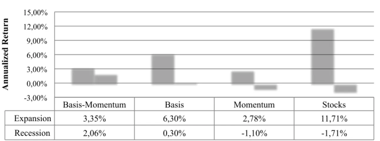
Bakshi, Gao and Rossi (2015) show that carry and momentum strategies are more profitable in recessions than expansions, being a good hedge against equity exposure during recession periods. To draw the same reasoning to the long-short portfolios of basis, momentum and basis-momentum I use the NBER Recession Indicators Series to find whether this is true. A performance table gives us the annualized returns for the three long-short trading strategies and exposure to U.S. stocks during expansion and recession periods. See Table 6:
Basis-Momentum Basis Momentum Stocks
Expansion 3,35% 6,30% 2,78% 11,71%
Recession 2,06% 0,30% -1,10% -1,71%
-3,00% 0,00% 3,00% 6,00% 9,00% 12,00% 15,00%
A
n
n
u
al
iz
ed
R
etu
rn
23 Focusing first on the momentum strategy, it performs poorly during recessions with an average monthly return of (−1.10%), while during expansions it has a 2.78% average monthly return. Basis strategy performs well during recessions, having a positive average month return of 0.30%. In expansion, it performs better that the momentum long-short portfolio, having an average return of 6.30%. This goes along with Bakshi, Gao and Rossi (2015) conclusions. Furthermore, my analysis reveals that the basis-momentum strategy is the best in hedging against stocks. In recessions, the average monthly return of the equity market is −1.71%, while the momentum has a positive return of 2.06%. This means, that the basis-momentum strategy more than hedges the loss in the stock market. During expansions, the basis-momentum has an average monthly return of 3.35%. In the second sample, the annualized returns, which can be seen in Table 7, give us unstable results during expansions. This means that we do not have a robustness that would encourage an investor to implement always the same strategy. However, the basis-momentum still continues to be the best strategy when comes to hedge against equity exposure, with a 2.06% annualized return during recessions relative to 0.25%, 2.27% and −1.74%, for Basis, Momentum and Stocks, respectively.
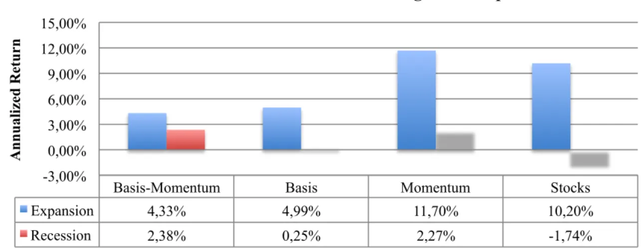
5.2 Liquidity Regime
The fed’s funds rate is an important guidance of the liquidity of the economy. Illiquidity regimes are considered to be the most defiant for investors21. It is important to note that when the Fed cuts the funds rate, it is usually because the economy needs incentives to recover for
21
See Ilmanen et al. (2014)
Basis-Momentum Basis Momentum Stocks
Expansion 4,33% 4,99% 11,70% 10,20%
Recession 2,38% 0,25% 2,27% -1,74%
-3,00% 0,00% 3,00% 6,00% 9,00% 12,00% 15,00%
A
n
n
u
al
iz
ed
R
etu
rn
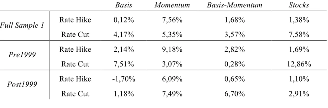
24 financial stress, while rate hikes avoids an inflationary regime caused by an expansion of the economy. Here, I want to see whether the trading strategies are able to give proper returns during such difficult regime. The Full Sample starts on February of 1985 to capture the full time series of the fed’s funds rate. Again, the long-short strategies (basis and basis-momentum) seem to perform better during times of financial distress, given by rate cut regime in Table 8, except for the long-short momentum strategy.
Table 8 – Basis, Momentum and Basis-Momentum high4 minus low4 during two
different liquidity regimes: The table shows the annualized monthly returns
Basis Momentum Basis-Momentum Stocks
Full Sample 1 Rate Hike 0,12% 7,56% 1,68% 1,38%
Rate Cut 4,17% 5,35% 3,57% 7,58%
Pre1999 Rate Hike 2,14% 9,18% 2,82% 1,69%
Rate Cut 7,51% 3,07% 0,28% 12,86%
Post1999 Rate Hike -1,70% 6,09% 0,65% 1,10%
Rate Cut 1,18% 7,49% 6,70% 2,91%
5.3 Inflation Regime
According to Ilamen et al. (2004), the most adverse regime is when there is raising inflation together with a recession. Here, I will study how the three trading strategies together with the equity market in four different scenarios. In the worse case scenario, with increasing inflation during an economic recession, the momentum and basis-momentum high4 minus low4 strategies give robust results, as they partially hedge losses in the equity market in full sample. This is true for the full sample, as well as the before and after 1999 subsamples. The same conclusion is made during recession periods with inflation below the fed’s inflation target of 2%22. The momentum and basis-momentum long-short strategies outperform the stocks market. When the economy is in expansion while inflation is increasing, the returns on the strategies and the equity market seem quite overvalued. On the other hand, when we have expansion together with a low inflation relative to the 2% fed’s target, none of the strategies can beat the equity market. However, the basis-momentum is the one who performs the best.
22
25
Table 9 – Basis, Momentum and Basis-Momentum Strategies during four different
inflation regimes: The table shows the annualized monthly returns.
Basis Momentum Basis-Momentum Stocks
Full Sample 1 Above target Inflation + Recession
0,41% 1,44% 1,35% -1,30%
Pre1999 -0,20% 0,16% 0,48% 0,40%
Post1999 1,06% 2,80% 2,26% -3,07%
Full Sample 1 Below target Inflation + Recession
-0,12% 0,57% 0,70% 0,15%
Pre1999 0,00% 0,00% 0,00% 0,00%
Post1999 -0,24% 1,18% 1,44% 0,30%
Full Sample 1 Above target Inflation + Expansion
5,95% 10,16% 1,82% 7,13%
Pre1999 12,65% 12,54% 2,86% 11,78%
Post1999 -0,62% 7,77% 0,76% 2,50%
Full Sample 1 Below target Inflation + Expansion
0,69% 0,37% 1,10% 2,80%
Pre1999 0,90% -0,05% 1,10% 2,71%
Post1999 0,15% 0,77% 2,06% 2,53%
5.4 Volatility Regime
The main focus here is to analyze how the trading strategies behave in a bearish and bullish market. I will use the CBOE’s VIX Index, available from January 1991, for the proxy of the state of the economy23. Usually, the VIX increases during financial stress (bearish market) and decreases when investors’ optimism increases (bullish market). Table 8 shows that in full sample momentum and basis-momentum long-short strategies tend to perform better in a bear market than in a bull market. In pre1999 subsample, this conclusion no longer holds, while in the post1999 subsample, these two strategies pay again high returns when investors need the most.
Table 10 - Basis, Momentum and Basis-Momentum Strategies during two different
volatility regimes: The table shows the annualized monthly returns.
Basis Momentum Basis-Momentum Stocks
Full Sample 1 Bearish -0,50% 7,62% 3,67% 2,46%
Bullish 4,61% 7,21% 0,26% 5,58%
Pre1999 Bearish 3,57% 4,34% 2,80% 5,92%
Bullish 9,49% 11,96% 3,80% 9,94%
Post1999 Bearish -2,35% 9,18% 4,09% 0,56%
Bullish 2,40% 5,06% 2,82% 3,43%
23
26
6
Conclusion
The systematic exposure in commodity futures market should be analyzed by including U.S., Europe and China’s signals, as the three countries show explanation power of the cross-variability of commodity future returns. Moreover, long-only commodity portfolios are also sturdily exposed to macroeconomic risk, while long-short commodity trading strategies seem to show little exposure to such systematic risk.
Throughout the paper I find that the investors’ market sentiment indicators play a strong role in explaining not only the individual commodity futures returns, but also only and long-short trading strategies, especially basis-momentum portfolio returns. I find that there is an asymmetric effect in sentiment signals, as they can strongly explain trading-strategies during recession periods.
Following long-short trading strategies give investors several advantages, which become clear by analyzing difficult possible scenarios in the economy. The NBER regime shows us that, during recessions, basis-momentum can fully hedge equity exposure. Furthermore, long short trading strategies, basis and basis-momentum strategies, perform better during financial distress periods, measured by lack of liquidity in the market. When FED is forced to cut rates to stimulate the economy, these two portfolios are capable of given strong returns. In the most challenging scenario for investors, given by increasingly inflation during a recession period, momentum and basis-momentum give investors positive results, as they can partially hedge equity exposure. Additionally, in a high equity market’s volatility regime, usually linked to a bearish market, momentum and basis-momentum perform better.
27
7
References
• Baker, M., and J. Wurgler. 2006. “Investor Sentiment and the Cross-Section of Stock Returns”, The Journal of Finance 61(4) 1645-1680
• Baker, M., and Jeffrey Wurgler. 2007. “Investor Sentiment in the Stock Market”,
Journal of Economic Perspectives 21(2) 129-152
• Bakshi, Gurdip, Xiaohui Gao and Alberto Rossi. 2015. “Understanding the Sources of Risk Underlying the Cross-Section of Commodity Returns”, Review of Financial Studies 28(5), 1428-1461
• Basu, Devraj, Roel C.A Oomen and Alexander Stremme. 2006. “How to time the Commodity Market”, Journal of Derivatives & Hedge Funds, Vol.16, No.1, pp. 1-8, 2010
• Boons, Martijn and Melissa Porras Prado. 2015. “Basis-Momentum”
• Casa, T. Della, M. Rechsteiner and A. Lehmann. 2009. “Facts and myths about commodity investing” – Research & Analysis Man Investments
• Erb, Claude B. and Campbell R. Harvey. 2006. “The Tactical and Strategic Value of Commodity Futures”
• Etula, Erkko. 2009. “Risk Appetite and Commodity Returns” – Harvard University
• Gargano, Antonio, Allan Timmermann. 2012. “Predictive Dynamics in Commodity Prices”, International Journal of Forecasting 30 (2014) 825-843
• Gao, Lin and Stephan Suss. 2015. “Market Sentiment in Commodity Futures Returns”
28
• Kat, Harry M. and Roel C.A Oomen. 2006. “What every investor should know about commodities PART I: Univariate Return Analysis” – Working paper
• Szymanowska, Marta, Frans de Roon, Theo Nijman and Rob Van der Goorbergh. 2013. “An Anatomy of Commodity Futures Returns”
• Miffre, Joelle and Adrian Fernandez-Perez. 2012. “The Case for Long-Short Commodity Investing: Performance, Volatility and Diversification Benefits”.
• Park, Peter, Oguz Tanrikulu and Guodong Wang. 2009. “Systematic Global Macro” – Graham Capital Management, L.P.
• Ribeiro, Ruy. 2009. “Economic and price signals for commodity allocation” – Global Asset Allocation & Alternative Investments J.P.Morgan
29 Annex 1 – D es cr ip ti ve A n al ys is for C ommod ity F u tu re s R etu rn s: T hi s t abl e is f or the f irs t ful l sa m pl e, from F ebrua ry of 1983 to F ebrua ry of 2014. T he c om m odi tie s fut ure s cont ra ct s are inc lude d int o groups . T he E ne rgy group inc lude s onl y the H ea ting O il cont ra ct ; the L ive st oc k group inc lude s the F ee de r Ca ttl e, L ive Ca ttl e and L ive H ogs c ont ra ct s; M et al s group inc lude G ol d, S ilve r and Coppe r cont ra ct s; O ils ee ds group inc lude S oybe an O il, S oybe ans M ea l a nd S oybe ans c ont ra ct s; S of ts grou p inc lude Cof fe e, O ra nge J ui ce a nd Coc oa cont ra ct s a nd Indus tri al M et al
s group i
nc lude Cot ton a nd L um be r c ont ra ct s.
Statistic Energy Livestock Metals Grains Oilseeds Softs Industrial9MaterialGCSI9Index CRB9Index Stocks
Nbr.9of9observations 373 373 373 373 373 373 373 373 373 373
Minimum D0,301 D0,133 D0,252 D0,222 D0,209 D0,185 D0,182 D0,278 D0,170 D0,218
Maximum 0,370 0,140 0,201 0,483 0,291 0,198 0,214 0,211 0,098 0,132
Range 0,671 0,274 0,453 0,705 0,500 0,384 0,396 0,489 0,268 0,349
1st9Quartile D0,044 D0,022 D0,026 D0,039 D0,033 D0,036 D0,037 D0,029 D0,011 D0,017
Median 0,008 0,002 0,002 D0,004 D0,001 D0,002 D0,003 0,004 0,002 0,011
3rd9Quartile 0,060 0,028 0,031 0,032 0,038 0,038 0,033 0,038 0,016 0,036
Mean 0,91% 0,12% 0,32% ,0,20% 0,39% ,0,03% ,0,24% 0,47% 0,23% 0,78%
Variance9(nD1) 0,008 0,001 0,003 0,005 0,004 0,003 0,003 0,003 0,001 0,002
Standard4deviation4(n,1) 8,90% 3,83% 5,40% 6,72% 6,55% 5,82% 5,89% 5,60% 2,59% 4,38%
Skewness9(Pearson) 0,379 D0,192 D0,236 1,059 0,189 0,000 0,061 D0,111 D0,677 D0,767
30 A n n ex 2 – D es cr ip ti ve A n al ys is for C ommod ity F u tu re s R etu rn s: T hi s ta bl e is f or the se cond ful l s am pl e, from M arc h 1991 to F eb rua ry 2014. T he E ne rgy group inc lude s H ea ting O il, Crude O il, G as ol ine , N at ura l G as a nd G as -O il P et rol eum c ont ra ct s; L ive st oc k group inc lude s F ee de r Ca ttl e, L ive Ca ttl e and L ive H ogs c ont ra ct s; M et al s group inc lude s G ol d, S ilve r and Coppe r cont ra ct s; the G ra ins group inc lude Corn, O at s, W he at and Ca nol a cont ra ct s; O ils ee ds inc lude s S oybe an, S oybe ans M ea l and S oybe ans c ont ra ct s; S of ts inc lude Cof fe e, O ra nge J ui ce , Coc oa a nd S uga r and Indus tri al M at eri al s group inc lude Cot ton and L um be r c ont ra ct s.
Statistic Energy Livestock Metals Grains Oilseeds Softs Industrial9MaterialGCSI9Index CRB9Index Stocks Bonds
Nbr.9of9observations 276 276 276 276 276 276 276 276 276 276 276
Minimum E0,274 E0,133 E0,252 E0,222 E0,178 E0,132 E0,182 E0,278 E0,170 E0,169 E0,011
Maximum 0,315 0,094 0,201 0,194 0,165 0,157 0,214 0,211 0,098 0,112 0,007
Range 0,589 0,228 0,453 0,416 0,343 0,289 0,396 0,489 0,268 0,281 0,018
1st9Quartile E0,038 E0,023 E0,022 E0,040 E0,026 E0,031 E0,042 E0,030 E0,011 E0,018 E0,002
Median 0,009 E0,001 0,005 E0,003 0,001 0,002 E0,005 0,009 0,003 0,011 0,000
31
Figure 1. Macroeconomic Index: Constructed by the first component of the PLS regression
32 F igu re 2 . Inve st ors S ent im ent c apt ure d by m ont hl y cha nge s in the L ea di ng Inde x and the Ba si s-M om ent um hi gh3 m inus l ow 4 m ont hl y re turns !10,00% !8,00% !6,00% !4,00% !2,00% 0,00% 2,00% 4,00% 6,00% 8,00% 10,00% 12,00%
1983% 1984% 1985% 1986% 1987% 1988% 1989% 1990% 1991% 1992% 1993% 1994% 1995% 1996% 1997% 1998% 1999% 2000% 2001% 2002% 2003% 2004% 2005% 2006% 2007% 2008% 2009% 2010% 2011% 2012% 2013%
33 A n n ex 3 – Corre la tion m at ri x f or the m ac roe conom ic va ri abl es : t hi s ta bl e is f or the f irs t f ul l sa m pl e, f rom F ebrua ry of 1983 t o F ebrua ry of 2014. Proximity)matrix)(Pearson)correlation)coefficient):
34 Annex 4 – Corre la tion m at ri x f or the m ac roe conom ic va ri abl es : thi s ta bl e is f or the s ec ond ful l s am pl e, f rom M arc
h 1991 t
o F
ebrua
ry 2014
Proximity)matrix)(Pearson)correlation)coefficient):