A Thesis presented as part of the requirements for the Degree of Doctor of Philosophy in Economics
Theory and Evidence on
Self-Fulfilling Sovereign Debt Crises
Sandra Maria Carvalho Vicente do Bernardo, nr. 518
A Thesis carried out on the Ph.D. in Economics program under the supervision of: Prof. Andr´e de Castro Silva
This work analyzes theoretically and empirically the potential self-fulfilling fea-tures of sovereign debt crisis. The theoretical model modifies Cole and Kehoe
(1996, 2000) by considering that the default is partial. In the model, there are debt limits within which self-fulfilling crises may occur. The numerical results show that, within the crisis zone, up to an intermediate debt level, the opti-mal government policy is to run down the debt until it reaches the safe limit to avoid higher borrowing costs. Above a certain amount, however, the government chooses to run up the debt, to avoid sharp reduction in government spending. The empirical investigation assesses the determinants of the probability of default in Portugal. The model builds onJeanne and Masson(2000) and is brought to Por-tuguese data using a Markov-switching regime framework. The results show that between 2000-14 two regimes subsisted: a tranquil and a crisis regime. The switch between regimes seems to be unrelated with macroeconomic fundamentals, which is interpreted as self-fulfilling jumps in the beliefs of credit markets.
I would like to express my gratitude to my advisor Prof. Andr´e Silva for his invaluable guidance, productive pressure, constructive criticism and friendly advice in the course of the work.
My deep gratitude also to Prof. Luis Catela Nunes, who willingly and patiently accepted to advise me on the specificity of the empirical chapter.
My warm thanks equally to Prof. Pedro Vicente for the renewed opportunity to develop this research.
Abstract . . . i
Acknowledgements . . . ii
Abbreviations . . . vi
List of Figures . . . vii
List of Tables . . . ix
Introductory note 1 1 Self-fulfilling Sovereign Debt Crises with Partial Default 3 1.1 Introduction. . . 3
1.2 Facts and background on sovereign defaults . . . 6
1.2.1 Some evidence on partial defaults. . . 6
1.2.2 Related literature. . . 12
1.3 The model. . . 16
1.3.1 Production function . . . 16
1.3.2 Consumers . . . 17
1.3.3 Government . . . 18
1.3.4 International bankers . . . 18
1.3.5 Debt zones . . . 19
1.3.6 Sunspot variable and market clearing . . . 19
1.3.7 Timing . . . 20
1.3.8 Recursive Markov Equilibrium . . . 21
1.4 Computation of the equilibria . . . 25
1.4.1 Optimal behavior of private agents . . . 25
1.4.2 Government behaviour . . . 29
1.4.3 Characterizing the zones. . . 35
1.4.4 Results . . . 38
1.5 Numerical computation . . . 40
1.5.1 Functions and parameters . . . 40
1.5.3 Limitations of the results . . . 50
1.6 Conclusion . . . 51
2 Market beliefs and fundamentals in the Portuguese sovereign debt crisis 53 2.1 Introduction. . . 53
2.2 Related literature . . . 57
2.2.1 Spillover effects . . . 57
2.2.2 Fundamentals and expectations . . . 60
2.2.3 Empirical methods . . . 61
2.3 The model. . . 63
2.3.1 Assumptions and setup . . . 63
2.3.2 Fundamental-based equilibria . . . 64
2.3.3 Sunspot equilibria . . . 65
2.3.4 Multiple equilibria and Markov-switching regimes. . . 66
2.4 Empirical strategy . . . 68
2.4.1 The dependent variable . . . 68
2.4.2 Fundamental variables . . . 70
2.4.3 Preliminary analysis of the model. . . 81
2.5 Model specification and estimation results . . . 88
2.5.1 Constant transition probabilities . . . 88
2.5.2 Time-varying transition probabilities . . . 91
2.5.3 Regime-varying coefficients . . . 93
2.5.4 Discussion of results . . . 96
2.5.5 Limitations of the results . . . 103
2.6 Conclusion . . . 104
References 106 Appendix 117 A Appendix of Chapter 1 117 A.1 Consumers problem . . . 117
A.1.1 Crisis zone with no previous default . . . 117
A.1.2 No default. . . 118
A.1.3 Default . . . 118
A.2 Government’s problem . . . 119
A.2.1 Default Zone . . . 119
A.2.3 Crisis zone . . . 123
A.2.4 Participation constraint . . . 128
A.3 MATLAB Code . . . 129
A.3.1 Steady state. . . 129
A.3.2 Code. . . 130
B Appendix of Chapter 2 137 B.1 Summary of empirical literature. . . 137
B.2 Data set description . . . 143
B.2.1 Debt sustainability . . . 143
B.2.2 External position . . . 144
B.2.3 Competitiveness . . . 145
B.2.4 Capacity to service the debt. . . 146
B.2.5 Risk and liquidity . . . 146
CDS Credit Default Swap
CTP Constant Transition Probability EC European Commission
ECB European Central Bank EU European Union
GDP Gross Domestic Product IMF International Monetary Fund MSR Markov Switching Regime REER Real Effective Exchange Rate RVC Regime Varying Coefficients
1.1 Defaults are partial I . . . 7
1.2 Defaults are partial II . . . 8
1.3 Yields on 10-years government bonds for selected European countries. . . 10
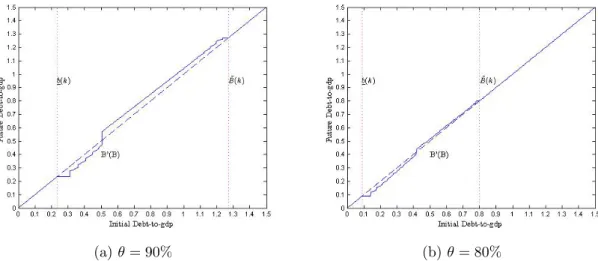
1.4 Debt paths . . . 38
1.5 Government debt policy function for full and partial default of 10%. . . 41
1.6 Bonds’ price in different zones . . . 42
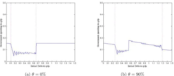
1.7 Government spending as ratio to GDP for full and partial default of 10% . . 43
1.8 Government debt policy function for different probabilities of default . . . 44
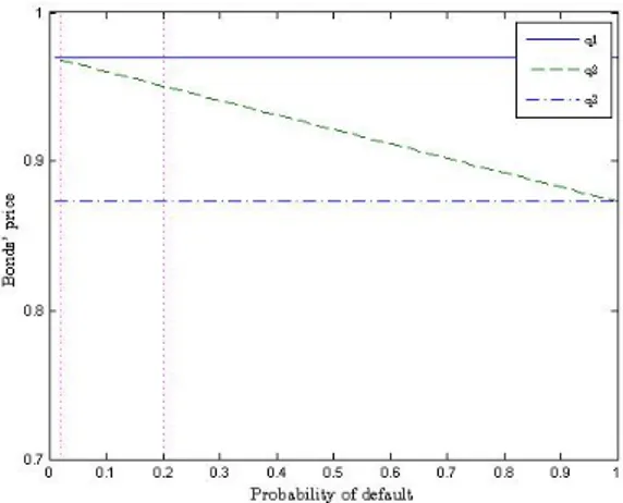
1.9 Relation between bonds’ price and the probability of default with θ= 90%. . 45
1.10 Government debt policy function for different recovery rates . . . 46
1.11 Relation between bonds’ price and the recovery rate with π= 2% . . . 46
1.12 Government debt policy function for different default penalties (Z) . . . 47
1.13 Government debt policy function for different tax rates (τ) . . . 48
1.14 Evolution of the value function and the recovery rate . . . 49
2.1 10-year Portuguese government bond spreads relative to German bonds . . . 54
2.2 Spreads 10-year government bond yields . . . 68
2.3 Portuguese sovereign debt spreads and differenced spreads . . . 69
2.4 Debt as % of GDP . . . 71
2.5 Scatter of spreads and debt as % of GDP . . . 71
2.6 Monthly debt as % of tax revenues and yearly tax revenues as % of GDP . . 72
2.7 General government deficit as percentage of GDP . . . 73
2.8 Current and capital account ratio to GDP . . . 74
2.9 Gross external debt ratio to GDP. . . 75
2.10 Real effective exchange rate and unit labour costs . . . 76
2.11 GDP year-on-year growth and unemployment rate . . . 77
2.12 Liquidity and international risk aversion . . . 78
2.13 Smoothed transition probabilities of being in a crisis regime: CTP . . . 90
2.14 Smoothed transition probabilities of being in a crisis regime: TVTP . . . 93
2.16 Smoothed transition probabilities of being in a crisis regime: RVC-TVTP . . 96
2.17 Timing of regime switch with constant-regime coefficients . . . 98
2.18 Timing of regime switch with regime-varying coefficients . . . 98
B.1 Comparison of monthly transformed and quarterly original debt as % of GDP 143 B.2 Deficit as percentage of GDP . . . 144
B.3 Monthly transformed and quarterly deficit as percentage of GDP . . . 144
B.4 Quarterly and monthly transformed external debt to GDP. . . 145
B.5 GDP year on year growth rate . . . 146
1.1 Default recovery rates, 1983-2013 . . . 9
1.2 Changes in output in selected defaulting countries . . . 10
1.3 External Debt at the Time of Default: Frequency Distribution, 1970-2001 . . 11
1.4 Parameters for Mexico at the end of 1994 . . . 40
2.1 Correlation between variables indebt sustainability group . . . 73
2.2 Correlation between variables inexternal position group . . . 75
2.3 Economic fundamentals variables . . . 79
2.4 Descriptive statistics . . . 80
2.5 Results of unit-root and stationarity tests . . . 81
2.6 OLS estimates . . . 82
2.7 Results of cointegration tests . . . 83
2.8 OLS, DOLS and FMOLS estimates . . . 84
2.9 VECM estimates of cointegrating relation . . . 85
2.10 MSR-CTP estimates . . . 89
2.11 MSR-TVTP estimates . . . 92
2.12 MSR with regime-varying coefficients - CTP estimates . . . 94
2.13 MSR with regime-varying coefficients - TVTP estimates . . . 95
2.14 Timing of regime switch in each MSR specification . . . 99
B.1 Summary of empirical literature on the determinants of sovereign bond yields in the euro area . . . 138
B.2 VECM short run estimates . . . 148
B.3 Selection of variables to include in TVTP in the specification in levels . . . . 150
B.4 Selection of variables to include in TVTP in the specification in differences . 150
B.5 Selection of variables to include in RVC-TVTP in the specification in levels . 151
This thesis addresses Theory and Evidence on Self-Fulfilling Sovereign Debt Crises. Its aim is to analyze the potential self-fulfilling features of sovereign debt crises, both theoretically and empirically, the former considering a partial default scenario and the latter observing the performance of the Portuguese economy.
The theoretical background are second generation crisis models, which are character-ized by their articulation of fundamentals and market expectations, in the sense that crises are ascribed either to the deterioration of economic conditions or to shifts in expectations. These models usually lead to multiple equilibria since, depending on expectations, similar macroeconomic fundamentals may lead the economy to a different equilibrium.
In the first chapter, a Dynamic Stochastic General Equilibrium (DSGE) model is pre-sented. The most significant agent of this theoretical model is a benevolent government in need to rollover the public debt. The model is an extension ofCole and Kehoe(1996,2000), but it considers the possibility of a partial rather than a total default. Additionally, it pos-tulates that following the partial default the country will maintain its access to international credit markets. This feature contrasts with CK’s model, in which the country is banned from international credit markets.
The model analyzes two debt thresholds: a lower safe limit, below which default is never the optimal decision, and a high sustainable limit, above which default is always optimal. In between these thresholds emerges a crisis zone, where self-fulfilling beliefs may condition the government’s decision to repay the debt. In this crisis zone, if creditors believe that the government will repay the public debt, they will be willing to lend at a lower price, thus allowing the debt rollover and ultimately helping to meet their initial expectations (of no default). If not, international credit will only be available at a higher price, thus contributing to default, again fulfilling the initial expectations (of default).
The second chapter is an empirical investigation of the determinants of the probability of default in Portugal from January 2000 until December 2014. The model builds onJeanne and Masson (2000) seminal paper on the self-fulfilling features of currency crisis and is brought to Portuguese data through a Markov-switching regime framework.
The main conclusions are outlined as follows: (i) during the period under analysis two regimes were identified - a tranquil regime, with low expected default rates and low bond yields, where favorable macroeconomic fundamentals are perceived as sustainable and thus self-fulfill low default expectations; and a crisis regime, with high expected default rates and high yields, where macroeconomic fundamentals are unfavorable thus favoring high proba-bility of default; (ii) the switch between regimes seems to be unrelated to macroeconomic fundamentals; (iii) the latter indicates that the debt crisis may have been, to some extent, self-fulfilling; indeed, a regime switch is interpreted as self-fulfilling jumps in the beliefs of creditors.
Self-fulfilling Sovereign Debt Crises
with Partial Default
1.1
Introduction
The recent euro area sovereign debt crisis has attracted renewed interest on the determi-nants of sovereign debt defaults, in particular on sustainable public debt limits and on the possibility that financial markets’ beliefs dominate economic fundamentals. Following Cole and Kehoe (1996, 2000), this work aims at finding circumstances in which sovereign debt crises may be self-fulling. In the model, these circumstances are related to the definition of debt limits, within which a self-fulfilling crisis may occur, and to the lenders’ expectations on the probability of default.
A self-fulfilling crisis may arise as a result of lenders beliefs on the government willingness to repay previous debt. Taking into account that public debt is exposed to the financial institutions’ disposition to accept government to roll over existing debt that has reached maturity, then if bankers do not lend, the country will default. Within this context, if bankers do not expect government to repay, they will not lend, thus conditioning the government’s decision in such a way that it becomes optimal to fulfill those expectations. So, if bankers assign a positive probability to a government default, it may indeed collapse a default on debt that would otherwise be repaid. Such default is expressed by a debt restructuring that results in a loss to creditors, either in the form of an outright default, a loss in face-value (write-off), or even a debt rescheduling.
partial default is the most common case: one of the findings of the cross-country historical review of public debt data from 1750 by Reinhart and Rogoff (2009, p. 61) is that most defaults are partial because, ”even if creditors do not have the leverage (from whatever source) to enforce full repayment, they typically have enough leverage to get at least something back”. Therefore, the CK model is modified by introducing the possibility of a partial default and by considering that, when public debt suffers a haircut of 1−θ, in subsequent periods the government is still able to issue new debt, although at a higher cost. The model is a general version of the original one, since ifθ= 0 the model becomes a complete default one.
The initial debt level is the crucial variable that determines the occurrence of a default. More specifically, and along the lines of CK, if the initial debt level is low enough, a default never occurs; on the contrary, if the debt level is sufficiently high, a default constitutes the optimal decision. The other possibility is the initial debt level falling in the crisis zone, wherein a self-fulfilling crisis may take place in case international bankers lend at a higher cost: if the country is depending on its ability to roll over debt contracts, such that it becomes vulnerable to an increase in the cost of borrowing, then if creditors lend at a higher price, the country will end up defaulting.
The definition of these debt thresholds is a relevant issue, since empirical literature has shown that defaults occur for almost any initial debt level. Reinhart and Rogoff(2009, p. 25) show that (i) external debt-to-GDP exceeded 100 percent in only 17 percent of the defaults or restructuring episodes; (ii) one half of all defaults occurred at levels below 60 percent; (iii) defaults took place against debt levels that were below 40 percent of GNP also in 17 percent of the cases.
After a default, as suggested by empirical evidence, significant downturns in economic activity take place. This feature is included in the model by means of a drop in productivity depending on the haircut fraction. Since private agents’ decisions depend on how much they believe productivity will be, the mere possibility of a default leads private agents to lower investment levels. Additionally, a default risk implies an increase in the cost of borrowing, stemming from an increase in the risk premium of bonds. In the model, if the debt level moves from the safe to the crisis zone, there is an increase in the cost of borrowing; after a default occurs, the cost further rises.
The model provides optimal policy decisions for the strategic benevolent government, which is vulnerable to speculative attacks on the part of non-strategic international bankers. The computation of debt thresholds is one of the main features of the model, because agents’ optimal decisions depend on which ”zone” where the initial debt is included. Moreover, since the model includes partial default to take place, it is possible to relate debt thresholds with the fraction of default. The main findings of the model are obtained through computational methods, using the CK model parameters. The results of the analytical and numerical calculations can be summarized as follows: (i) when in the crisis zone, in order to avoid the costs of a default, the government has an incentive to run down the debt positions until it leaves the crisis zone; (ii) However, above a certain intermediate level the incentive is to run up the debt, avoiding sharp reduction in government spending; (iii) if the cost of default is low , the crisis zone narrows down and there is an incentive not to reduce the debt level at all.
1.2
Facts and background on sovereign defaults
1.2.1 Some evidence on partial defaults
This section provides evidence of some facts related to defaults that support some as-sumptions of the model. Notwithstanding, the first question that needs to be addressed is what comprises a default. Even though there are several definitions, it is possible to assess a common aspect: a sovereign debt default occurs when, as the result of a change in the contract initial conditions, the creditor incurs in a loss. The most obvious forms of default are outright defaults, when the government repudiates the debt payment, and debt write-off, which corresponds to a reduction in the face-value of debt. Besides these situations, debt rescheduling may also be considered a default, if it results in a loss to creditors, as considered byReinhart and Rogoff (2009).
A specification of the type of events that constitute a sovereign default is provided by
Moody’s (2014, p. 4). Accordingly, a default occurs when there is: (i) a missed or delayed disbursement of interest or principal payment; (ii) a distressed exchange whereby (1) an obligor offers creditors a new or restructured debt, or a new package of securities, cash or assets that amount to a diminished financial obligation relative to the original obligation; and (2) the exchange has the effect of allowing the obligor to avoid a payment default in the future; or as defined in credit agreements and indentures; (iii) a change in the payment terms of a credit agreement or indenture imposed by the sovereign that results in a diminished financial obligation, such as a forced currency re-denomination (imposed by the debtor, himself, or his sovereign) or a forced change in some other aspect of the original promise, such as indexation or maturity.
Alternatively, Arellano, Mateos-Planas and Rios-Rull (2013) define a partial default as the fraction of payments missed, which is different from a debt haircut: ”Debt haircuts are generally measured as the fraction of the value of debt in arrears that lenders lose after renegotiations. Partial default (...) measures the fraction of bonds in arrears.”
Herein, we consider that a default occurs whenever the creditor recovers less than the complete amount it was initially agreed. This recovery rate is hardly 0%, which would constitute a complete default. In fact, a partial default is the most common situation and, indeed, several empirical studies find no evidence of complete default. Cruces and Trebesch
(2013) construct a database of sovereign debt defaults (haircuts) with foreign banks and bondholders from 1970 until 2010, covering 180 cases in 68 countries. The haircut is computed as the percentage difference between the present values of old and new instruments, discounted at market rates prevailing immediately after the exchange. The authors find that the average sovereign haircut is 37%; that there is a large variation in haircut size (one half of the haircuts are below 23% or above 53%); and that the average haircuts have increased over the last decades. Figure 1.1 depicts how sovereign debt haircuts are distributed over time and countries, showing that no episode of a complete default was found in the sample.
Figure 1.1: Defaults are partial I Source: Cruces and Trebesch(2013)
Figure 1.1also shows that the haircut on rescheduling episodes is on average lower than the haircut resulting from debt restructuring. Within the 180 episodes, there were 123 pure rescheduling, with a mean haircut of 24%, while the remaining 57 restructurings also involved face-value reduction and had a much higher mean of 65%.
Arellano, Mateos-Planas and Rios-Rull (2013) corroborate this perspective and, by ex-tendingCruces and Trebesch (2013) panel to 99 developing countries from 1970-2010, they document that countries often have some debt outstanding payments and that default is al-ways partial. The definition of a default here is different: default-to-debt ratio in Figure1.2
Figure 1.2: Defaults are partial II
Source: Arellano, Mateos-Planas and Rios-Rull(2013)
.
In this study, countries default on average on 22% of total liabilities and they have positive arrears about 53% of the time. In this latter case, the average default increases to 50% and countries continue to service the debt, paying about 4% of output and continue to borrow about 1.7% of output.
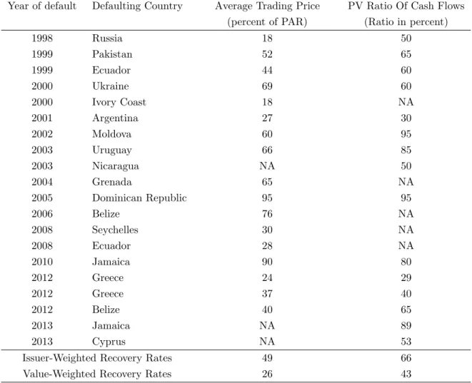
Moody’s(2014), covering data from 1983-2013 among 124 Moody’s-rated sovereigns, pro-vide average recovery rates both and value-weighted. The distinction between issuer-and value-weighted averages is important because smaller countries are more likely to default, thus potentially inflating issuer-weighted default rates.
Table 1.1: Default recovery rates, 1983-2013
Year of default Defaulting Country Average Trading Price PV Ratio Of Cash Flows (percent of PAR) (Ratio in percent)
1998 Russia 18 50
1999 Pakistan 52 65
1999 Ecuador 44 60
2000 Ukraine 69 60
2000 Ivory Coast 18 NA
2001 Argentina 27 30
2002 Moldova 60 95
2003 Uruguay 66 85
2003 Nicaragua NA 50
2004 Grenada 65 NA
2005 Dominican Republic 95 95
2006 Belize 76 NA
2008 Seychelles 30 NA
2008 Ecuador 28 NA
2010 Jamaica 90 80
2012 Greece 24 29
2012 Greece 37 40
2012 Belize 40 65
2013 Jamaica NA 89
2013 Cyprus NA 53
Issuer-Weighted Recovery Rates 49 66
Value-Weighted Recovery Rates 26 43
Source: Moody’s(2014)
Table 1.2: Changes in output in selected defaulting countries
Country Default episode Deviation from trend:
(starting date) Output Consumption Investment
Argentina 2001Q4 -11.2 -11.4 -44.2
Ecuador 1999Q3 -6.0 -15.1 -25.1
Indonesia 1998Q2 -7.6 -18.1 -16.3
Mexico 1982Q3 -3.1 -4.9 -21.8
Peru 1980Q1 -3.7 -8.7 -25.7
Peru 1983Q1 -8.4 -10.0 -12.9
Philippines 1983Q4 -7.7 -9.6 -39.1
Russia 1998Q4 -10.8 -10.6 -38.3
South Africa 1985Q3 -2.1 -8.1 -8.2
South Africa 1989Q4 1.5 -1.3 6.4
Average -5.9 -9.8 -22.5
Source: Pe˜na(2012)
All cases are characterized by a decrease in output and consumption, with the largest decline observed in investment dynamics: average output and consumption deviations from trend range roughly between−6% and−10% , respectively, while their investment counter-part varies by as much as 22.5% below trend.
These findings are in line withMendoza and Yue(2012), who conclude that defaults are associated with an average GDP and consumption fall about 5% below trend and a labor fall to a level about 15% lower than in the three years prior to the defaults.
Another important feature related to debt defaults is its relation to interest rate spreads, since these reflect the probability that investors assign to a crisis. Taking as an example the yields of euro area peripheral countries’ sovereign bonds from 2008, shown in Figure1.3, we observe that these yields started to move apart from German yields, considered risk-free bonds.
In fact, the relation between the haircut fraction 1−θ and the probability of default can be assessed from the Credit Default Swap (CDS) spread. If, for simplicity, we consider a 1-year CDS spread (premium), then the default probability can be estimated as (Deutch Research Bank,2015):
π = CDS Spread 1−θ
E.g., if the recovery rate is 40%, a spread of 200 bp would translate into an implied probability of default of 3.3%. Even though the implied market probability of default for a sovereign bond can be calculated from yield spreads and a fixed rate of recovery,Blundell-Wignall and Slovik(2011) point out that the fixed rate of recovery assumption may constitute a difficulty, since this changes over time and over countries.
The estimation of the probability of default based on interest rates spreads is the core of empirical literature aiming at analyzing the role of market sentiments in European sovereign debt crisis. BothBruneau, Delatte and Fouquau(2014) andde Grauwe and Ji (2013), using different econometric procedures, show that both the fundamentals and ”animal spirits” ignited the European sovereign crisis.
Finally, with regards to the initial debt level, the crucial variable in the model, that conditions whether the country is vulnerable to a self-fulfilling crisis, there is mixed evidence on its relevance. On the one hand, Mendoza and Yue (2012) identify initial high external indebtedness for countries that default on sovereign debt, on the other hand, Reinhart and Rogoff(2009) show that defaults occur for any debt level, as is shown in Table 1.3.
Table 1.3: External Debt at the Time of Default: Frequency Distribution, 1970-2001
External debt-to-GNP range at Percent of defaults or restructuring
the first year of default or restructuring in middle income countries
Below 40 17
41 to 60 30
61 to 80 23
81 to 100 13
Above 100 17
To summarize, Aguiar and Amador (2015) survey and list the following key finding re-garding empirical facts related to defaults:
i Concerning defaults and its aftermath: defaults happen with regularity throughout his-tory; defaults often occur in bad times, but with exceptions; defaults involve a heteroge-neous pattern of ”haircuts”; defaults generate a period of lengthy renegotiation;
ii Concerning evidence on bond spreads: on average spreads over US bonds are higher for longer maturity bonds, and while all spreads increase during crises, the short-term bond spread increases relatively more; emerging market bond yields exhibit significant co-movement, suggesting that global factors explain a large fraction of the common variation in spreads;
iii Successful growth episodes are associated with low and declining levels of foreign indebt-edness.
1.2.2 Related literature
This work relates to the literature on self-fulfilling debt crisis and to the definition of sustainable debt limits. The termself-fulfilling belief captures rational outcomes not related to economic fundamentals, such as preferences, endowments or technology. This feature is modelled by specifying a state of confidence that is assumed to take one of two sunspot-driven values, e.g., normal and high. Typically these models produce multiple equilibria -sunspots, and the choice of the equilibrium situation depend on the ”random” confidence. Romer(2011, p. 296) identifies a sunspot equilibrium when some variable that has no inherent effect on the economy matters because agents believe that it does. Any model with multiple equilibria has the potential for sunspots: if agents believe that the economy will be at one equilibrium when the extraneous variable takes on a normal value and at another when it takes on high value, then agents’ behave in ways that validate this belief.
The incorporation self-fulfilling beliefs in economics literature is attributed to Azariadis
The expansion of self-fulfilling sovereign debt crisis literature1 has often been motivated by specific episodes. Alesina, Prati and Tabellini (1990) perform an analogy of public debt runs to bank runs based on confidence sentiments and inspired by Italian debt management policies pursued in the 1980s. Building an infinite horizon model, close to the CK model, they find two equilibria outcomes depending on the costs of default: (i) a ”good” equilibrium where investors buy new debt and government is able to roll over forever; (ii) a ”bad” equilibrium where investors do not lend, because they think other investors will act the same way, and thus the government is forced to default. Moreover, they conclude that if foreign governments or international institutions could act as lenders of last resort, it would increase the chance of a country hit by debt panic to survive without defaulting.
Cole and Kehoe (1996, 2000), motivated by the Mexico’s 1994-95 debt crisis, conciliate self-fulling debt crises with debt ceilings’ literature, which aims at finding the highest level of debt that potential creditors can lend without triggering a default (Obstfeld and Rogoff,
1996, p. 381-8). Their research builds upon a DSGE model in order to identify the optimal debt policy depending on the initial debt level: below the lower bound the government never defaults even if creditors do not lend; above the upper bound the government defaults even if creditors lend; within those limits lies the crisis zone, where a crisis may occur with positive probability (included as a proxy for the market participants’ beliefs). In the crisis zone, market participants’ beliefs (probability of default) select the equilibrium outcome and, if a default does not occur, the government finds it optimal to reduce debt level so as to leave the zone. These thresholds depend on the level of private capital stock and on the level of government debt, but also on its maturity: even with a low debt to GDP ratio, short-maturity debt plays an important role on whether a crisis may take place. The government optimal decision is to leave the crisis zone, by reducing the debt level or by increasing debt maturity. It is worth mentioning that this type of crisis results from a coordination failure2 among
private lenders. Suppose that a subset of creditors becomes pessimistic about the possibility of default and decides not to lend. If there exist sufficiently strong strategic complementarities
3 in the economy, then it is in the other creditors’ best interest not to lend as well. As a
result, borrowers’ expectations of a default are validated, which in turn causes an output decrease without any change in economic fundamentals. According to Chamon (2007) this possibility could be eliminated. In fact, at least when there is a single borrower (like the government) such crises could be prevented by mechanisms which allow investors to bid 1Tularam and Subramanian(2013) survey financial cries literature and highlight the fact that each model was adapted to specific situations to explain the financial crises faced rather than being visionary or systematic
in approach;Aguiar and Amador(2015) review the theoretical literature on sovereign debt; andTomz and
Wright(2013) review the empirical research on sovereign debt and default. 2SeeRomer(2011, chap. 6) on coordination failure models.
3
on new bonds contingent on the resulting issue, inducing investors to lend because they expect other investors to so. Moreover, providing that the country satisfies the investors’ participation constraint, it can choose any outcome for that issue, being able to select the ”good equilibrium”.
Araujo, Leon and Santos(2013) extend CK model to discuss alternative currency regimes (dollarization, local currency and common currency) for countries that are highly dependent on international lending. The model does not explicitly model inflation, exchange rate and monetary policy. Instead, the authors summarize the consequences of the currency devalu-ation in terms of the purchasing power of a currency, which they refer as a partial default, in the sense that, after devaluation, the bond issued in local or in common currency will not have the same value, in real terms, as before. To compare local currency regime with dollarization, they also include domestic debt, thus making it possible to inflate away the domestic debt to avoid the external debt default. Their numerical findings perform a welfare analysis for Argentina and Brazil during the 1998-2001 period, in order to understand the reason why those countries were under different regimes between 1998 and 2001.
A second extension concerns nominal bonds. Aguiar et al.(2013) extend the CK model to nominal debt in an environment in which the government chooses the inflation rate subject to a utility cost of high inflation, which proxies for the government’s commitment to low inflation. They show that issuing nominal bonds has an ambiguous effect on the vulnerability to a self-fulfilling debt crisis. Specifically, if the government’s commitment to low inflation is high absent a crisis, then nominal bonds have a desirable state-contingent feature; in good times, the real return is high, while in the event of a crisis, the government inflates away part of the real value of the bonds. As creditors prefer partial repayment to outright default, the ability to respond with inflation generates a superior outcome to real bonds. However, if the commitment to low inflation is weak even in good times, the government loses the state-contingency potentially allowed by nominal bonds. In particular, the government has a temptation to inflate ex post even in normal times, and this will be reflected in lower bond prices (or higher interest rates) ex ante, making repayment much more burdensome. This effect may be large enough to dominate, generating a larger crisis zone for nominal bonds.
Aguiar et al. (2013) use this fact to rationalize why many emerging markets with weak in stationary regimes issue bonds in foreign currency, while economies like the US, the UK, and Japan issue large amounts of domestic currency bonds at low nominal interest rates and seemingly without risk of self-fulfilling crises.
govern-ment’s incentive to default by making the safe level of government debt very low. The model is calibrated to match the Argentinian 2001-2002 crisis.
The euro area debt crisis motivated further research, particularly related to recessions and bailouts. Conesa and Kehoe(2012) extended the original CK model by considering that the economy may be in normal times or in a recession. If the economy is facing a recession with a positive probability of recovery, then governments may find it optimal to keep bor-rowing, expecting that a recovery will increase its revenues. This ”gambling for redemption” behavior leads to increasing debt levels, which, if the recession persists, inevitably causes default. Again, the authors define debt thresholds where self-fulfilling crises are possible, and characterize conditions (i) under which gambling for redemption is the optimal policy, and (ii) under which the optimal policy is to reduce debt level and exit the crisis zone.
Conesa and Kehoe (2014) further extended model by adding a probability of bailout. However, their results indicate that a very large penalty on interest rate is needed to induce the government to run down its debt after a bailout, thus turning the bailout unattractive.
In a related research applied to the euro area sovereign debt crisis, Arellano, Conesa and Kehoe (2012) conclude that under high interest rates on government bonds and high costs of default, governments have incentives to reduce its debt and avoid sovereign default. On the contrary, low interest rates and low costs of default provide incentives for a government to gamble for redemption. In particular, and within the European debt crisis, the authors conclude that the EC, ECB and IMF intervention, by lowering the cost of borrowing and reducing default penalties, are encouraging euro area governments to gamble for redemption.
Adler and Lizarazo(2015) focus on the role of domestic banks as the major governments’ borrowing source. Using a small open economy DSGE model, he explores the fact that self-fulfilling crisis may stem from government over borrowing in domestic banks (which borrow abroad), thus linking bank solvency to fiscal solvency and leaving the economy vulnerable to market expectations.
Durdu, Nunes and Sapriza (2013) rationalize self-fulfilling crisis through the incorpo-ration of news. They analyze the extent to which changes in expectations due to policy announcements or news in general matter for macroeconomic fluctuations across countries. The authors find that negative news can lead to a default, even if current output is high. In fact, negative news about future fundamentals increases next period’s default risk, which raises the cost of borrowing. As it becomes more onerous to roll over debt, it may trigger a default in the current period.
1.3
The model
The model includes three types of agents - consumers, government and international bankers - and one type of good, used both for consumption and investment in each period t= 1,2, ....
The framework isCole and Kehoe(1996,2000) standard DSGE model with capital accu-mulation, which includes a benevolent government that provides a valued public good. The provision of this good is financed through a (fixed) tax on household’s income and through public debt. Debt matures in periodt+ 1 and the government does not commit to its repay-ment. We modify CK model by considering the possibility of default being partial 0< θ <1, instead of always complete,θ= 0.
Consumers are risk neutral and do not access international credit markets, but they save assets in the form of capital, thus they are less willing to substitute consumption over time. The inclusion of capital is related to the fact that a reduction in domestic investment may change the government incentives to honor its debt.
1.3.1 Production function
Production utilizes capital and, implicitly, inelastically supplied labor:
y(Kt, θt) =Z1−θt
·f(Kt), (1.3.1)
whereKt denotes the aggregate or economy-wide stock of capital andf(Kt) is continuously differentiable, concave, monotonically increasing function, satisfying f(0) = 0, f′(0) = ∞
andf′(∞) = 0. The parameter 0< Z <1 corresponds to the drop in GDP when the country
defaults and θt ∈[0,1] represents the fraction of upcoming debt repayed in period t. Hence 1−θtis the haircut imposed on the owners of government debt, such thatθ= 1 corresponds to a full repayment and θ= 0 to a full default. In what follows we are considering that the government options are not to default or to default on a pre-determinedθ= ¯θ, thus actually θt∈
0,θ¯ .
Whenever the country defaults, there is a permanent reduction in output and the higher is the haircut, 1−θ >¯ 1−θ, the lower is the output level,Z1−θ¯< Z1−θ. The assumption that the default penalty is proportional to output is proposed by Sachs (1984) and by Cohen and Sachs (1986)cit in. Obstfeld and Rogoff (1996, p. 351). Alternatively, Corsetti and Dedola
Adam and Grill (2013) show that it is optimal for a fully committed government to occasionally deviate from the legal repayment obligation and to repay debt only partially. This holds true even if default generates significant deadweight costs ex-post.
This default penalty can be rationalized by two reasons. On one hand, a default may be accompanied by ”direct punishment” from creditors, which may impose trade sanctions (e.g., confiscation of exports or imports in transit, seizure of trade-related foreign assets or limited access to short-term trade credits) that prevent the country from seizing the gains from trade (Obstfeld and Rogoff, 1996, p. 351). On the other hand, a default involves a reputation damage, which prevents the country from accessing international capital markets, thus generating a credit crunch. Cole and Kehoe (1998) analyse reputation spillover effects.
1.3.2 Consumers
A continuum of measure one, infinitely living consumers derive utility from private con-sumption, ct, and from government consumption , gt. The representative household maxi-mizes the following additively time separable lifetime utility function:
U(ct, gt) =E0 ∞
X
t=0
βt[c
t+v(gt)]. (1.3.2)
The utility includes a linear function of private consumption and a function v(gt) of government spending, that is continuous, differentiable, strictly concave and increasing and v(0) = −∞. Since the consumers are risk neutral in their own consumption, we ignore the possibility of their borrowing from, or lending to, the international bankers. If instead, consumers were risk averse they could be induced by their future income risk to accumulate assets in the form both of capital and, especially, of savings with the international bankers. However, this would substantially complicate the analysis without changing the essential features of the analysis (Cole and Kehoe,2000, p. 93-4).
Consumers’ budget constraint is:
ct+kt+1 ≤(1−τ)·[y(kt, θt)−δ·kt] +kt, (1.3.3)
where 0 < τ < 1 is the constant proportional tax on domestic income after depreciation. Thus, consumers disposable income is a fraction, 1−τ, of domestic income and the amount of capital stock carried out from the previous period, which is used to consume domestically produced goods,ct, and to invest in domestic capital, kt+1.
1.3.3 Government
Government is benevolent, in the sense that it maximizes consumers’ utility, U(ct, gt), subject to its own budget constraint:
gt+θt·Bt≤τ ·[y(Kt, θt)−δ·Kt] +qt·Bt+1. (1.3.4)
In each period the government sells new debt, Bt+1, at price qt and repays 1 unit for due debt if the decision is not to default or repaysθt in case it decides to default. As we will see, the price of one-period government bonds depends on the amount of bonds the government offers to sell and on the (arbitrary) probability that a crisis occurs if the economy is in the self-fulfilling crisis zone. If the government defaults on debt repayments, then in subsequent periods there is a drop in output andqt decreases permanently.
1.3.4 International bankers
A continuum of measure one, risk neutral, infinitely living international bankers derive utility from their private consumption, xt:
UIB(xt) =E0 ∞
X
t=0
βtxt, (1.3.5)
Bankers’ risk neutrality captures the idea that the domestic economy is small compared to world financial markets. Each banker is endowed with ¯x in each period and chooses how many new government bonds to purchase. The price that bankers are willing to pay for these bonds, qt, depend on their expectations regarding government default decision in the next period.
International bankers budget constraint is:
xt+qt·bt+1 ≤x¯+θt·bt. (1.3.6)
1.3.5 Debt zones
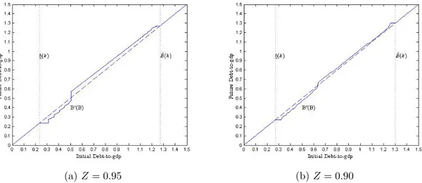
We consider the existence of three debt zones where the following outcomes are possible: if the current level of debt is in the ”no crisis zone”, the government never defaults; in the crises zones, a self fulfilling debt crisis may occur, and in the ”default zone”, where a default has already occurred. These zones are limited by the following debt thresholds:
❼ b(Kt;θt), which corresponds to the highest level of debt where no crisis occurs givenKt. This threshold is called the ”upper safe debt limit” or the ”lower limit for a no-lending continuation condition”. If Bt ≤ b, the government fully repays even if bankers lend at a higher price; alternatively, if Bt> b, the government defaults if bankers lend at a higher price; otherwise it does not default.
❼ B¯(Kt;π, θt), which defines the lowest level of debt for which default occurs. This threshold is also referred to as ”upper sustainable debt limit” or the ”upper limit for a participation constraint”. If Bt≤B¯, the government repays if bankers lend at a lower price; otherwise it defaults.
The crisis zone lies between those debt levels, where a crisis may occur depending on the confidence that international bankers have on government not defaulting. Cole and Kehoe
(2000) showed that in the case θ ∈ {0,1}, then b(Kt)<B¯(Kt;π). Notice that the limits of the crisis zone depend onB,K and θ, but within the crisis zone the probability of a crisis π is independent on the levels ofB,K and θ.
1.3.6 Sunspot variable and market clearing
To model the sunspot, we consider that in each period, if the country is in the crisis zone, a random variable ζ is drawn from the uniform distribution [0,1]. The realization of this variable determines the equilibrium outcome:
❼ If ζ < π, then bankers expect a default and lend at a higher price, thus triggering a default and the crisis turns out to be self-fulfilling;
❼ If ζ ≥ π, then the risk that bankers assign to a crisis, and a consequential default, doesn’t prevent them from buying additional bonds at a lower price and a crisis does not occur.
Because ζ is uniformly distributed on the unit interval, π is both the crucial value of ζ, and the probability thatζ < π (Da-Rocha, Gim´enez and Lores, 2013, p. 20). It should be noted that the realization of the sunspot variable is only relevant inside the crisis zone. In fact,πcorresponds to the probability that the sunspot variable takes on a value that indicates the international creditors to panic if a crisis would be self-fulfilling.
The market-clearing condition for the government debt is bt+1 = Bt+1. For consumer’s
individual capital stock the condition iskt+1 = Kt+1, where kt+1 is the individual decision
andKt+1 is the aggregate value.
1.3.7 Timing
The timing of actions within each period, and the fact that the government is the only strategic agent, makes it possible to consider the effects of each decision on the future debt price, upcoming government revenue and the level of private consumption. Agents choose their actions sequentially as follows (Cole and Kehoe,1996,2000):
1. The sunspot variable,ζt, is realized and the aggregate state is St= (Bt, Kt, θt−1, ζt);
2. The government chooses how much new debt,Bt+1, to sell taking bonds’ price,qt(st, Bt+1),
as given;
3. Bankers choose whether to purchase new debt,bt+1, at price,qt;
4. The government decides whether to default, θt ∈
0,θ¯ , and how much to spend on the public good, gt;
5. Consumers choosect and kt+1.
The importance of the timing of actions is highlighted by Ayres et al. (2014) and Teles
the borrower chooses current debt or debt at maturity; borrower moves first and chooses current debt (which is the case herein considered). However, if the borrower moves first and chooses debt at maturity, there is a single equilibrium.
It is also worth noting that the price of debt depends on the amount of new debt, Bt+1,
but the decision on whether to default depend on the amount of debt to be repaid,Bt.
1.3.8 Recursive Markov Equilibrium
The recursive-markov equilibrium here described is characterized by the following features: (i) the government cannot commit itself to repay previous debt or to follow a given debt or spending path; (ii) within each period, agents sequentially choose their actions, in the order previously described.
A recursive competitive equilibrium is characterized by time invariant functions of a lim-ited number of state variables, which summarize the effects of past decisions and current information (Mehra,2008). These functions include (a) a list of value functions Vc,Vg and Vg, where the superscript denotes the agent; (b) a price function ψ
q(·); (c) policy functions specifying agents’ decisions: for consumersC(·), for the governmentB(·),G(·) and Θ(·); (d) and a law of motion for capital stock,κ(·). The adjective Markov denotes that the equilibrium decision rules depend only on the current values of the state variables, not their histories. Per-fect means that the equilibrium is constructed by backward induction and therefore builds in optimizing behaviour for each agent for all conceivable future states (Ljungqvist and Sargent,
2012, p. 185). In fact, backwards induction is the appropriate procedure, because it allows agents to be aware of other agents’ optimal decisions. This way, an optimal time-consistent policy can be found to account for the possibility of confidence crises, encouraged through the limited commitment assumption (Cole and Kehoe,2000, p. 92).
At the beginning of each period, the aggregate state of the economy is defined as S = (B, K, θ−1, ζ). Taking into consideration this information, other variables that affect each
agent’s maximization problem and its state in a future period, determines the current state of an agent. The solution to an agent’s maximization can be found with respect to its indi-vidual state, and expressed through a value function, maximizing the agent’s utility, and a policy function, leading to this maximized utility through the optimal selection of its choice variables. In summary, the following functions are being derived within the recursive equi-librium: consumers value function Vc(k, S, B′, g, θ) and its policy functions C(k, S, B′, g, θ)
and κ(k, S, B′, g, θ); the government’s value function Vg(S) and its policy functions B′(S),
Θ(S, B′, q) and G(S, B′, q); the bankers’ value function Vb(b, S, B′) and its policy function
b′(b, S, B′); the bond price function ψq(S, B′) and an equation of motion for the aggregate
In what follows, subscripts denote the variable with respect to which the derivative is taken, a prime in a variable indicates next-period values, and a prime in a function indicates it is evaluated at next-period variables. Since we use backwards induction, we start with consumers’ problem because they move last.
Consumers move last, by choosing c and k′, at a time where all other decisions are
known. So, consumers know their own capital holdings, k, the government decisions B′, g
andθ, the price that international bankers pay for new debt, q, and the sunspot, ζ, which is only relevant when the debt level in within the crisis zone. Moreover, in subsequent periods, they expect government to follow the policiesG(·), B(·) and Θ(·), all yet to be defined.
The representative consumer’s value function is defined by the functional equation:
Vc(k, S, B′, g, θ) = max
c,k′ {U(c, g) +β·EV
c(k′, S′, B′(S′), g′, θ′)}
subject to c+k′ ≤(1−τ)·[y(k, θ)−δ·k] +k c, k′ ≥0
S′= (B′, κ′, θ, ζ′)
g′ =G(S′, B′(S′), ψ
q(S′, B′(S′)) θ′ = Θ(S′, B′(S′), ψ
q(S′, B′(S′))
(1.3.7)
Since in equilibriumk=K, the consumption optimal decision function can be expressed asc = C(k, S, B′, g, θ) and the economy-wide stock of capital is expected to evolve
accord-ing to K′ =κ(k, S, B′, g, θ) derived from the budget constraint. The production function is
y(k, θ) =f(k) if θ−1=θ= 1 and isy(k, θ) =Z1−θ·f(k), otherwise.
Vg(S, g, θ) = max g,θ
U(c, g) +β·EVg(S′, g′, θ′)
subject to g+θ·B ≤τ ·[y(K, θ)−δ·K] +q·B′
c=C(K, S, B′, g, θ)
S′= (B′, K′, θ, ζ′)
K′ =κ(k, S, B′, g, θ)
g≥0 θ∈ h0,1i
(1.3.8)
The resulting optimal public purchases and default policy function can be expressed as G=G(S, B′, q) and θ= Θ(S, B′, q). The default decision will affect the level of output and,
through the budget constraint, the level of public spending.
International bankers take as given bond its own holdings, b, and government new debt,B′, to solve the functional equation:
Vb(b, S, B′) = max
b′ {x+β·EV
b(b′, S′, B′(S′))}
subject to x+ψq(S, B′)·b′ ≤x¯+ Θ(K, B, ζ)·b
S′= (B′, K′, θ, ζ′)
K′=κ(k, S, B′, g, θ)
b≥ −A¯
(1.3.9)
Since bankers are risk neutral, and behave competitively, they buy all the bonds offered by the government, as long as ¯x is sufficiently large and the price function of new bonds is ψq(S, B′).
Vg(S) = max
B′ {U[c, g] +β·EV g(S′)}
subject to S′= (B′, K′, θ, ζ′)
c=C(k, S, B′, g, θ)
K′=κ(k, S, B′, g, θ)
g=G(S, B′, ψq(S, B′))
θ= Θ(S, B′, ψq(S, B′))
(1.3.10)
The solution to this problem isB′ =B(S). Notice, however, that the government cannot
commit to repay upcoming due debt and if bankers do not lend, a default occurs, even if the government has decided not to default.
1.4
Computation of the equilibria
The derivation of the equilibrium involves severel specificities. The first feature arises from the discontinuity of bonds’ prices, caused by the debt thresholds. As no constant price for public debt holds, the government’s value function has kinks which directly affect its policy function. The second factor is related to the limited commitment assumption, as the government is not able to commit for future policy choices, the manual derivation of a continuous value function becomes impossible (Madison,2012, p.29). Moreover, we consider that the default decision is taken in only one period.
The current level of government debt is the crucial determinant of consumers, bankers, and government decisions (Cole and Kehoe,1996). If the level of debt is low enough so that the government would pay it even if it were unable to sell new debt, then no crisis is possible. Consumers choose a high level of capital; bankers do not demand a risk premium on the return to government bonds; and government maintains a high constant spending level with low constant debt level. If, on the other extreme, the level of debt is high enough that the government would default even if it could sell new debt at a lower price, then consumers choose a low level of capital; bankers buy government debt at a lower price; and the government maintains a low constant spending level with high constant debt level.
In between these two extremes lies the crisis zone. Here self-fulfilling debt crises can occur with fairly arbitrary probability. Consumers choose a level of capital that decreases with higher probability of a crisis; bankers demand a risk premium from the government; and the government may choose to reduce its spending to run down its debt and eventually leave the crisis zone or, if the debt reduction is too costly, it may choose to run up the debt until it defaults, to avoid a sharp reduction in spendings..
1.4.1 Optimal behavior of private agents
The optimal decisions of consumers and bankers depend on their believes about next period output level, which in turn may depend on probability they assign to the government defaulting in the next period. So, in the no-crisis zone private agents expect θ = 1; in the default zone, they expectθ= ¯θ; in the crisis zone, these agents expectθ= 1 with probability π and they expect θ = ¯θ with probability 1−π. We now can characterize consumers’ and bankers’ behavior and then infer the transition function for capital k′ and price function
1.4.1.1 Consumers
As previously mentioned, consumers do not behave strategically and their decision de-pends on the expectations for next period output. In this section, to find a stationary steady state, we followCole and Kehoe(1996) procedure, which evolves using variational methods4. Henceforward, we denotecn,kn,cθ and kθ as consumption and capital levels contingent on government not defaulting or defaulting in the next period. Moreover, we take into consideration that according to the timing of actions, consumers move after knowing the current government decision, and that the default penalty occurs in the same period of the default decision. In equilibrium, individual choiceskcoincide with aggregate choicesK. The rules henceforth presented are derived in AppendixA.1.
Expectations of a crisis
In the crisis zone, given a constant probability of a crisis taking place, the value of the sunspot variable determines the outcome. Here, if default has not occurred until period t, consumers assign a probability π to a default and a probability 1−π to no default. The representative consumer, givenkt, knt+2 and kθt+2 chooses ct, kt+1 and cnt+1, cθt+1, where the
former correspond to the choices of consumption in periodst+1 contingent on the government not defaulting or defaulting, respectively. Thus, consumers’ solve the variational problem:
max ct,kt+1,cn
t+1,c
θ
t+1
ct+β·(1−π)·ctn+1+β·π·cθt+1
subject to
ct≤(1−τ)·[y(kt,1)−δ·kt] +kt−kt+1
cnt+1 ≤(1−τ)·[y(kt+1,1)−δ·kt+1] +kt+1−ktn+2
cθt+1 ≤(1−τ)·
y(kt+1,θ¯)−δ·kt+1
+kt+1−kθt+2
ct, cnt+1, cθt+1, kt+1 ≥0
(1.4.1)
The FOC of the consumers problem imply that investment is stationary at the level kπ determined by the rule:
1 =β·h(1−τ)nf′(kπ)·h(1−π) +π·Z1−θi−δo+ 1i (1.4.2)
4Variational methods are used to find the stationary state of a dynamic problem. ”The basic technique is
The household’s Euler equation has the usual interpretation: to attain maximum utility, consumers’ must be indifferent between consuming one more unit today and the expected present value of saving and consuming that unit in the future. The additional term (1− π) + π ·Z1−θ < 1 arises because the representative agent internalizes the fact that the possibility of a crisis leads to a lower output. Once the stationary state capital stock is determined, consumers’ budget constraint (1.3.3) can be used to determine the stationary value of consumption. In period t, k (chosen in t−1) may be different from kπ. Thus, consumption, if no default has occurred int:
cπ(k) = (1−τ)·[f(k)−δ·k] +k−kπ, (1.4.3)
As stated byCole and Kehoe (2000, p. 99) ”It is here that the risk neutrality of utility in consumption plays its role: if consumers are risk averse, then optimal investment and consumption are not stationary.”
Expectations of default
If consumers expect a default of θ = ¯θ in the next period, such that they expect the productivity parameter to be equal toZ1−θ¯, then the optimal level of capital accumulation, kθ, is derived from rule:
1 =β·n(1−τ)·hZ1−θ¯·f′(kθ)−δi+ 1o. (1.4.4)
The consumption level is set according to:
cθ(k) = (1−τ)·hZ1−θ¯·f(k)−δ·ki+k−kθ (1.4.5)
In particular, if the debt level is high enough, such that the economy is in the default zone, then a default has already occurred and consumers expect default as the only possible outcome, so the consumption level,cθ(kθ), evolves according to:
cθ(kθ) = (1−τ)·hZ·f(kθ)−δ·kθi (1.4.6)
Expectations of no default
Analogously, if consumers expect a full repayment, θ = 1, and that the productivity parameter is 1, then next period’s capital stock knsatisfies:
1 =β·
(1−τ)·
f′(kn)−δ
In this case, the consumption level is cn(k) is:
cn(k) = (1−τ)·[f(k)−δ·k] +k−kn (1.4.8)
Notice that the strict concavity off(k) implies that kn> kπ > kθ.
1.4.1.2 International bankers
The price function for bondsq(b′, θ) is the solution of the international bankers’ dynamic
programming problem (1.3.9). The resulting equation defines the price as the risk neutral discount rate of an international banker, β, adjusted by the expected value of a country’s default.
q(b′, θ) =β·E(θ′) (1.4.9)
Bankers’ risk neutrality and competitive behaviour imply that they are relatively passive, in the sense that, as long as the price of bonds satisfies Eq. (1.4.9), they buy all the debt the government offers. Since the bonds’ price depends on the expectations of default, which in turn depend on the zone where the initial deb level is included, then the debt thresholds cause breaks in the price of bonds.
Taking the debt thresholds as given, in the no-crisis zone bankers setq =β; in the default zone bankers setq =β·θ; finally, in the crisis zone, the realization of the sunspot variable rules the lending decision, such that ζ > 1 −π indicates a forthcoming crisis, such that bankers as well increase the price they demand for rolling over the government’s debt into a future period.
Thus the price of bonds is:
q(B′, θ) =
β ifB′ ≤b
β·(1−π) +β·π·θ ifb < B′ ≤B¯
β·θ otherwise
(1.4.10)
punished by markets tomorrow.
Unlike the CK model, here when a default occurs, bankers pay a lower price for next period’s debt, but the country is still allowed to borrow. When we set θ = 0, where a full default takes place, the country is permanently banned from international capital markets because it will not borrow at zero price. Finally, notice that the realization of the sunspot variable is only relevant inside the crises zone.
1.4.2 Government behaviour
In this section, we characterize the government’s payoffs and optimal policies in each of the three situations: default, no-default and crisis zone. Herein, we show that for sufficiently low debt levels, it is optimal for the government to repay even if bankers do not lend, and for sufficiently high debt levels, it is optimal to default, even if agents do not expect it.
In what follows, we denote gi(B, B′, q, k) and Vi(B, k), i = n, θ as the government’s spending and payoff functions of not defaulting and defaulting.
1.4.2.1 Default zone
In this situation, we consider thatB0≥B¯(kθ), such that the initial debt level lie in a zone
where a default is the only expected outcome. Thus,q =β·θ and the government solves the variational problem defined in (1.4.11), by choosing gt, gt+1 and Bt+1, and taking as given
Bt,Bt+2,kt andkt+1. In period t+ 1 the government defaults on its choice forBt+1.
max gt,gt+1,Bt+1
βt·v(gt) +βt+1·v(gt+1)
subject to
gt+Bt≤τ · h
Z1−θ·f(k
t)−δ·kt i
+β·θ·Bt+1
gt+1+θ·Bt+1 ≤τ·
h
Z1−θ·f(k
t+1)−δ·kt+1
i
+β·θ·Bt+2
gt, gt+1≥0
Bt+1≥B¯(kt) lim
T→∞(β·θ)
T ·B
t+T = 0
(1.4.11)
Appendix A.2.1 includes the computation of the general case where k0 6= kθ. Here, we
assume thatk0 =kθ, consumers set k=k′=kθ and c=cθ(kθ), such that the constant debt
level is:
Bθ(B0, kθ) =
1
Even though there is a constant debt level, there is a reduction in relation to the initial level. If this reduction falls bellow ¯B(kπ), as we will see from the policy in the crisis zone, the debt level will turn out to be ¯B(kπ).
The government average constant spending level is:
gθ=τ ·hZ1−θ·f(kθ)−δ·kθi− 1−β·θ
1 +β·(1−θ)·B0 (1.4.13)
The government’s payoff in this situation is:
Vθ(B
0, kθ) =cθ(kθ) +v
h gθ(B
0, Bθ, kθ)
i
+β· 1 1−β ·
n
cθ(kθ) +vhgθ(Bθ, Bθ, kθ)io (1.4.14)
In this zone, the payoff of defaulting is higher than rather not defaulting. In fact, given private agents decisions in this zone (q = β·θ, c =cθ(kθ) and k′ = kθ), if the government does not default it setsB1 =B0, such that:
gnθ=τ·hZ1−θ·f(kθ)−δ·kθi−(1−β·θ)·B
0 (1.4.15)
which is smaller than Eq. (1.4.13).
1.4.2.2 No default zone
Analogously, to derive the government policy in the no-crisis zone, we assume that B0 ≤
b(k0) and thatB1 ≤b(kn), that is, the initial and subsequent debt levels fall in the no-crisis
zone, such that since no crisis is possible (π = 0), thenq=β and θ= 1.
In this zone, the government solves the variational problem (1.4.16), by choosinggt,gt+1
andBt+1, and taking Bt,Bt+2,kt andkt+1 as given.
max gt,gt+1,Bt+1
βt·v(gt) +βt+1·v(gt+1)
subject to
gt+Bt≤τ ·[f(kt)−δ·kt] +β·Bt+1
gt+1+Bt+1 ≤τ ·[f(kt+1)−δ·kt+1] +β·Bt+2
gt, gt+1≥0
Bt+1≤b(kt)
lim T→∞β
T ·Bt
+T = 0
(1.4.16)
henceBt+2 =Bt+1.
When we assume that k0 = kn (the general case of k0 6= kn is in Appendix A.2.2), if
after bankers have lent the government’s decision is not to default, then B1 = B0 and the
government constant spending level is:
gn(B0, B0, kn) =τ ·[f(kn)−δ·kn]−(1−β)·B0 (1.4.17)
The government’s payoff of not defaulting is:
Vn(B
0, kn) =
1 1−β · {c
n(kn) +v[gn(B
0, B0, kn)]}. (1.4.18)
To see that in this zone the payoff of not defaulting is higher than the payoff of defaulting, we characterize an hypothetical situation where the government decides to default onB0after
bankers have lentB1. In periodtbankers had setq=β and consumers setk=kn,c=cn(kn)
and k′ = kθ. In subsequent periods, and even for low debt levels, the government faces a higher risk premium on debt issuing,q =β·θ, and a lower output level, both because of the default penalty and because consumers set capital at a lower level.
The value function of defaulting in the no-default zone Vθn is:
Vθn(B0, kn) =cθ(kn) +v[gθ(B0, B1, kn)] +
β 1−β ·
n
cθ(kθ) +v[gθ(B1, B1, kθ)
o
with
gθn(B0, B1, kn) =τ ·[Z1−θ·f(kn)−δ·kn]−θ·B0+β·B1
cθ(kn) = (1−τ)·hZ1−θ·f(kn)−δ·kni+kn−kθ
gθ(B1, B1, kθ) =τ ·[Z1−θ·f(kθ)−δ·kθ]−(1−β·θ)·B1
cθ(kθ) = (1−τ)·hZ1−θ·f(kθ)−δ·kθi. B1 =
θ
1 +β·(1−θ)·B0
(1.4.19)
Using the same procedure as in AppendixA.2.2 to find the constant debt level, we find:
Bθn(B0, kn) =
θ
1 +β·(1−θ)·B0+
+ 1−β
1 +β·(1−θ) ·τ· nh
Z1−θ·f(kθ)−δ·kθi−hZ1−θ·f(kn)−δ·knio.
1.4.2.3 Crisis zone
Herein, we assume that k0 = kπ and b(kn) < B0 ≤ B¯(kπ, π), that is the participation
constraint does not bind, such that the government wants to honor the current lending contract given that it is able to issue new debt. Sinceb(kn)> b(kπ) thenB
0 > b(kπ) and the
government faces the following choices in period 0:
1. plan to run debt down in T periods tob(kn) or less in T periods if no crisis occurs
2. plan to run debt up in W periods to ¯B(kθ, π) or less in W periods if no crisis occurs
3. never run the debt down and keep a constant debt level;
4. default now and afterwards keep a constant debt level.
After determining the governments’ payoff for each of these choices, the optimal decision corresponds to the option that offers the maximum payoff. In this section we find these governments’ policies. In section 1.5, we show that the optimal decision up to intermediate debt levels is to run down debt until it reaches the no-crisis zone, but for larger debt levels within the crisis zone, heavier government spending cuts change the incentive to reduce debt towards defaulting, even assuming a future higher borrowing cost.
Run debt down in T periods Under the conjecture that there was no previous default, private agents set c = cπ(k), k′ = kπ and q = β ·(1−π) +β·π ·θ, which we denote by
ˆ
β. The government plans to run debt down to b(kn) in T periods, instead of the standard spending smoothing policy, because it ends up receiving more when it sells less debt, since in the no-crisis zone q = β. When running down debt in T periods, the level of spending, derived in AppendixA.2.3, is constant atg=gT(B
0) and set to:
gT(B0) =τ·[f(kπ)−δ·kπ] + ˆβT−1·
1−βˆ
1−βˆT ·β·b(k
n)− 1−βˆ
1−βˆT ·B0 (1.4.20)
SettingBT < b(kn) cannot be optimal since it lowersgT and, by definition of T,BT−1 >