URBAN CHANGE MONITORING USING
GIS AND REMOTE SENSING TOOLS IN
KATHMANDU VALLEY (NEPAL)
URBAN CHANGE MONITORING USING GIS AND REMOTE SENSING TOOLS IN KATHMANDU VALLEY (NEPAL)
Dissertation supervised by:
Professor Pedro Cabral, Ph.D.
Dissertation co-supervised by:
Professor Mário Caetano, Ph.D.
Professor Filiberto Pla, Ph.D.
ACKNOWLEDGMENTS
Foremost, I would like to express my sincere gratitude to my supervisor, Prof. Dr.
Pedro Cabral, for his continuous support to successfully completing my thesis and
for his motivation, enthusiasm, and immense knowledge that added considerably to
my academic experience. I appreciate for his assistance in this matter.
Equally, I would like to thank the rest of my thesis committee members, Prof. Dr.
Mário Caetano, and Prof. Dr. Filiberto Pla for their encouragement, insightful
comments, and assistance they provided during the thesis period. I would like to
thank Prof. Dr. Marco Painho for taking time out from his busy schedule to guide us
to streamline our theses since the beginning.
Very special thanks go out to Prof. Dr. Werner Kuhn, Dr. Christoph Brox and all
concerned personality for giving me the academic direction, technical support as well
as every means to support my study. I must also acknowledge my Nepali colleagues
Deepak Kharal, Rabinra Maharjan, Prem Paudel, Pem Kandel and Roshan Sherchan
for their stimulating suggestion, guidance and help to further my academic career.
My office elders Deepak Joshi, Jagannath Koirala, Chewan Guragain, Kiran Dongol
and other office members also provided me a lot of help related to this study. At this
point, I would also like to memorize my pleasant times that I had with my colleagues
during the course in Europe.
In conclusion, I would like to consider here the continuous encouragement and
support I received from every member of my family throughout my studies and
appreciate my wife Srijana and sons Sardul and Srijal particularly for their patients
URBAN CHANGE MONITORING USING GIS AND REMOTE SENSING TOOLS IN KATHMANDU VALLEY (NEPAL)
ABSTRACT
The urbanization pattern during the period of 1989 to 2006 of Kathmandu valley was
studied using Landsat data. The main aims of the study were to apply Geographic
Information Systems (GIS) and Remote Sensing tools for the study of land use and
land cover classification, change analysis and urban growth model for 2019 of the
Kathmandu valley. The study also reviewed population growth and urbanization
trends in connection with increasing built up areas leading to the environmental
degradation. The population growth and urbanization trend of Kathmandu valley was
the highest among other cities in Nepal. Principal component analysis was applied to
spectrally enhance images to get the better image classification results. Images were
classified in six land use and land cover classes using supervised classification and
maximum likelihood algorithm which were then re-classed into built up and
non-built up to focus on urbanization. The analysis showed that the non-built up area had
grown up to 134% in 2006 since 1989. The assessed overall accuracies for the
classification of three images were between 86 to 89 percentages. Cellular Automata
Markov (CA_MARKOV) and GEOMOD modeling programs were used to project
the 2006 and then 2019 land use and land cover classes. The 2019 land use and land
covers was projected after satisfactory validation of projected 2006 land classes
resulting with Kappa more than 0.55 up to 0.75. The future projection of land classes
did not show that the urban growth will have significant effects to the designated
areas. However, there will be some effects in water bodies. The Landsat images
KEYWORDS
Geographic Information System
Kathmandu valley
Land use & cover change model
Remote Sensing
ACRONYMS
AHP – Analytical Hierarchy Process
CA – Cellular Automata
CBS – Central Bureau of Statistics
CR – Consistency ratio
DoS – Depart of Survey
ESRI – Environmental Systems Research Institute
ETM+– Enhanced Thematic Mapper Plus
GCPs – Ground Control Points
GIS – Geographic Information System(s)
GoN – Government of Nepal
ICIMOD – International Centre for Integrated Mountain Development
LUCC – Land Use Cover Change
MCE – Multi-Criteria-Evaluation
MoEST – Ministry of Environment, Science, and Technology
SLC – Scan-line corrector
SRTM –Shuttle Radar Topographic Mission
UNEP – United Nations Environment Programme
VDC – Village Development Committee
TABLE OF CONTENTS
ACKNOWLEDGMENTS ... iii
ABSTRACT ... iv
KEYWORDS ... v
ACRONYMS ... vi
1. INTRODUCTION ... 1
1.1. Background ... 1
1.2. Problem statement ... 2
1.3. Study area ... 4
1.4. Objectives ... 7
1.5. Research questions ... 7
1.6. Structure of the thesis ... 7
2. URBANIZATION OF NEPAL AND KATHMANDU VALLEY ... 9
2.1. Introduction ... 9
2.2. Evolution of urban areas ... 9
2.3. Demographic situation of Kathmandu valley ... 11
2.4. Causes of population growth in Kathmandu valley ... 13
2.5. Impact of tourism ... 15
2.6. Discussion ... 15
3. DATA AND METHODS ... 17
3.1. Introduction ... 17
3.2. Data ... 18
3.3. Software used ... 19
3.4. Image classification and accuracy assessment process ... 20
3.5. Land use and cover change modeling and validation ... 23
3.6. Discussion ... 25
4. RESULTS ... 26
4.1. Introduction ... 26
4.2. Image classification ... 26
4.2.2. Image classification ... 29
4.2.3. Accuracy assessment ... 31
4.2.4. Change analysis ... 34
4.3. Land use and cover change modeling ... 36
4.3.1. Model calibration ... 36
4.3.2. Model execution ... 45
4.3.3. Model validation ... 47
4.3.4. Urban land use prediction for 2019 ... 49
4.3.5. Implication of the urban growth ... 55
5. CONCLUSIONS ... 57
5.1. Discussion ... 57
5.2. Limitations ... 58
5.3. Future work ... 59
BIBLIOGRAPHIC REFERENCES ... 60
APPENDICES ... 64
1. Classification result of Mahalanobis distance ... 65
2. Classification result of Minimum distance ... 66
LIST OF TABLES
Table 1: Percent distribution of urban population and places by geographical region
... 10
Table 2: Level of urbanization by geographical region ... 10
Table 3: Distribution of population by district ... 11
Table 4: Population density by district ... 11
Table 5: Urban population growth trend ... 12
Table 6: Average annual growth rates of urban and rural population ... 12
Table 7: Detail characteristics of the Landsat imageries ... 19
Table 8: Land use class types of class areas ... 30
Table 9: Overall accuracy and Kappa (κ) statistics for the classifications ... 31
Table 10: Producer's and User's accuracy for individual land classes ... 32
Table 11: Land use re-class and areas ... 33
Table 12: Area change in hectare and percentage of land classes ... 34
Table 13: Area change in hectare and percentage of land re-classes ... 35
Table 14: Criteria to standardize fuzzy module ... 40
Table 15: Factor weights derived from AHP ... 42
Table 16: Cross-tabulation of land use 1999 (columns) against land use 2006 (rows) ... 44
Table 17: Area of predicted land classes for 2006 ... 47
Table 18: Kappa statistics for validation results ... 48
Table 19: Area of simulated maps of 2019 and true 2006 land re-classes ... 50
Table 20: Cross-tabulation of land use 1999 (columns) against land use 2006 (rows) ... 50
Table 21: Comparison area statistics of classified and projected maps ... 53
Table 22: Kappa statistics for validation results ... 53
Table 23: Comparison statistics of true and projection maps ... 54
LIST OF FIGURES
Figure 1: Study area ... 5
Figure 2: Kathmandu valley in 3D perspective [Band: 3, 2, 1] ... 6
Figure 3: Structure of thesis ... 8
Figure 4: Flow chart of image classification process ... 17
Figure 5: Flow chart showing land use projection calibration method ... 18
Figure 6: Composite bands of 1989, 1999 and 2006 images showing study area in yellow square [True color] ... 27
Figure 7: Spectrally enhanced 1989, 1999 and 2006 images of the study area ... 28
Figure 8: An example of training samples taken in an image ... 28
Figure 9: Land use land cover classification maps of Kathmandu valley ... 29
Figure 10: Bar chart land use quantization in 1989, 1999 and 2006 ... 30
Figure 11: An example for test samples taken in an image ... 31
Figure 12: Land use re-classification maps of Kathmandu valley ... 33
Figure 13: Bar chart land use quantization in 1989, 1999 and 2006 ... 34
Figure 14: Cross classification of Built up and Non-built up land classes ... 36
Figure 15: Constraints used to create suitability maps for urban growth ... 38
Figure 16: Factor maps showing range of suitability to urban growth ... 41
Figure 17: Analytical Hierarchy Process (AHP) ratings and Consistency ratio ... 42
Figure 18: Suitability maps showing high to low range of suitability to urban growth ... 43
Figure 19: Suitability maps showing range of land use change suitability from 1999 into 2006 ... 45
Figure 20: Built up and Non-built up land class projection for 2006 ... 46
Figure 21: Simulated Built up and Non-built up land class maps for 2019 ... 49
Figure 22: Suitability maps showing range of land change suitability from 1999 into 2006 ... 51
Figure 23: Comparison of true 2006 land class map with projection 2006 and 2019 maps of Kathmandu valley ... 52
Figure 24: comparison of true 2006 land re-class map with projection 2006 and 2019 land re-class maps ... 54
1. INTRODUCTION
1.1. Background
Urban change is the result of urbanization process. Urbanization, in general, is
known as the process of growth in the proportion of population residing in urban
places (CBS1, 2003a). This is characterized by higher population growth within the
city as well as migration of people from outside areas mainly rural to urban. The
urbanization process also involves the increase in number of urban fringes.
Agricultural land is continuously being converted to urban uses in the process of
urbanization all over the world (Pradhan, Perera, 2005). Therefore, rural areas get
urbanized as their economy become less and less dependent upon agriculture. In
summary, we can say that demography and land use pattern change, industrialization
and social transformation occur during the urbanization processes.
In recent decades, a diversified and growing economy has continuously attracted new
residents and stimulated significant urban growth (Yuan, Bauer, 2007). About half of
the world's current population is urban and total urban population also increased
threefold between 1950 and 1990 (Thouret, 1999). According to Pradhan, Perera
(2005), 2 billion new residents being added to the cities of the developing world in
the next 25 years and industrial development will continue putting pressure on land
use and environment in the major city areas. In the developing countries, large cities
are growing at a higher rate than those in the rest of the world (Thouret, 1999). This
means that 21st century will be the century of rapid urbanization (Pradhan, Perera,
2005).
The environmental condition of Kathmandu valley was very healthy endowed with
rich forests and scenic beauty, improved river basin, and lower pollution with clean
air. The soil is still very fertile as the valley is considered the site of an ancient huge
1
lake. In the previous decades, the farmers knowingly or unknowingly practiced the
organic farming with the adoption of agro-ecosystem (Baniya, 2008). However
nowadays, the scenario has been completely reversed as the resources and
environmental condition degraded badly due to rapid population growth. Therefore,
there is immediate need for proper planning of the Kathmandu valley valuing the
land resources for economic and environmental sustainability of the city
This may require more advanced spatial techniques supported by the policy makers
involving shifting of emphasis from basic geographic data handling into
manipulation, analysis and modeling in order to solve the real problem
(Ramachandran, 2010). In recent decades, remotely sensed data have been widely
used to provide the land use/cover information such as degradation level of forests
and wetlands, rate of urbanization and other human-induced changes (Alrababah,
Alhamad, 2006). Moreover, the advent of widely available and less expensive
Landsat imagery has permitted the development of highly accurate land cover map
products (Goetz, et. al., 2009).
The urban dynamics model driven by Geographic Information Systems (GIS) as well
as remote sensing data proved to be useful for identifying urban growth and land
use/cover tendencies that enable local planning authorities to recognize and manage
city growth according to the environmental carrying capacity, present and envisaged
infrastructure availability (Alameida et. al. 2005) as well as socioeconomic
considerations.
1.2. Problem statement
The cities in Kathmandu valley are expanding improper way because of rapid
population growth. As a consequence, there is a rising demand of land for residential
use. Between 1984 and 1998, large numbers of hectares of fertile and productive
sand, soil, and stone (ICIMOD2, MoEST/GoN3, UNEP4, 2007). There has been a
dramatic change in its land use composition during the periods 1984-1994 and
1994-2000 (Pradhan, Perera, 2005). Improper urban development caused an adverse
impact not only on agriculture and other land but also on the environmental condition
and the livelihoods of the area in the long run.
Due to its geography land is a scarce resource in Kathmandu valley and therefore has
to be used cautiously for its optimization and environmental sustainability (Pant,
Dongol, 2009). Moreover it is highly desirable to realize and access the real
uncontrolled urban situation and its impacts on different important land use/cover to
initiate the measures as early as possible to improve the environmental condition of
Kathmandu valley. However, the extensive expansion of urban centers over
agricultural land is being poorly monitored due to the ill-equipped land monitoring
system (Setiawan, Mathieu, Thompson-Fawcett, 2006).
This calls for planned development for the urban area and vicinities to minimize
these problems and needs up-to-date information on the land use/cover and
population of the Kathmandu valley. Therefore the study is intended to use GIS and
Remote Sensing tools to acquire the information from Landsat images for providing
knowledge on the trend of land utilization and urban growth that can be useful for
assessing the effects on sensitive areas and planning unmanaged urban growth in the
Kathmandu valley.
2
ICIMOD (International Center for Integrated Mountain Development) is a regional knowledge development and learning centre serving the eight regional member countries of the Hindu Kush-Himalayas – Afghanistan, Bangladesh, Bhutan, China, India, Myanmar, Nepal, and Pakistan .
3
MoEST/GoN (Ministry of Environment, Science and Technology, Government of Nepal) is the government agency in Nepal to promote research and development of science and technology and environmental sustainability in the country.
4
1.3. Study area
Recently Nepal is in the process of formulating new constitution. In anticipation of
the finalization and promulgation of the new constitution, Nepal has been politically
divided into 5 development regions, 14 zones and 75 administrative districts. Each of
these divisions has headquarters. Kathmandu valley is overall headquarters of the
country. Districts are further sub-divided into village development committees
(VDC) and municipalities. Currently, there are 3,914 VDCs and 58 municipalities.
Nepal is also divided into Plains, Hills, and Mountains respectively from South to
North as broad ecological zones.
Kathmandu Valley is the capital of Nepal, a country of highest peak known as the
Mount Everest in the world. The valley is bowl shaped and positioned between 270
32' 13" to 270 49' 10" N latitude and 850 11' 31" to 850 31' 38" E longitude. It is at a
mean elevation of about 1300 meters (4265 feet) above sea level (Pant, Dongol,
2009). It comprises three districts namely Kathmandu, Lalitpur and Bhaktapur.
Dhading, Kavrepalanchok, Nuwakot, Makawanpur and Sindhupalchok are the
(DoS,5 1999; ESRI online,6 2009)
Figure 1: Study area
High sandstone mountain ranges stand all around these districts such as Phulchowki
in the South East, Chandragiri/Champa Devi in the South West, Shivapuri in the
North West, and Nagarkot in the North East (Figure 2). The altitude of these
mountains varies around 1500 meters to 2800 meters (Baniya, 2008). The three
major river systems in the valley are the Bagmati, Bishnumati, and Manohara. There
are lakes and ponds also in all three districts.
5
( Landsat, 2006)
Figure 2: Kathmandu valley in 3D perspective [Band: 3, 2, 1]
Ancient history of the Kathmandu valley says that it was a huge lake which was
settled after draining away all the water through Chobhar gorge by a Chinese Saint.
Early settlements were around very few places. Townships developed and flourished
through Indo-Nepal-Tibet trade. Though many small towns were established by the
second century A.D. and urban centers by the 11th century, according to the records,
urbanization of the valley commenced in the late 1950s, accelerating during the
1970s. According to the population census of 2001, Kathmandu district had the
biggest urban population and the highest number of households in Nepal (Zurick,
1.4. Objectives
The main aim of this research was to apply GIS and Remote Sensing tools for the
attainment of the following objectives:
• To use Landsat images for the study of land use classification and analyze land use change of Kathmandu valley
• To know the amount of conversion of other land into urban land in
different dates and model urban change pattern of Kathmandu valley
1.5. Research questions
The study was focused to answer the following research questions:
• What was the trend of population growth and its distribution?
• What were the land use classes/practices in the city?
• Which land use classes were mostly used for urban growth?
• What are the future trends of urban growth and which areas are most suitable for urban expansion?
• Are GIS, Remote Sensing tools by means of Landsat images and other
data adequate and useful for this kind of study?
1.6. Structure of the thesis
The following chart is the brief structure of the thesis that shows flow of
Problem statement Study area
Chapter one Objectives
Research questions
Urbanization &
demographic status Chapter two
Input data sets 1989, 1999, 2006
Classification
Land use classes 1989, 1999, 2006
Classification accuracy?
Evaluation
Change detection
Model calibration, execution & validation
Projection 2019
Results & discussions
Chapter three
Chapter four
Conclusions &
future work Chapter five
2. URBANIZATION OF NEPAL AND KATHMANDU VALLEY
2.1. Introduction
The trend of demographic situation and urbanization process in Nepal particularly in
Kathmandu valley has been discussed in this chapter. The evolution of urban areas
and its trends in the major cities in different geographic location of Nepal in compare
to Kathmandu valley were the major concerns of the chapter. Since the thesis was
focused to study urbanization, it became important to study the causes of population
growth and urbanization trends in the Kathmandu valley. To solve the problems of
causes and effects of urbanization, GIS and remote sensing techniques have been the
suitable tools to perform the study.
2.2. Evolution of urban areas
Urban expansion has been occurring outside the Kathmandu valley only after
eradication of malaria in 1960s (Pant in Akhtar et. al, 2009) and construction of
highways along the country. Nepal had only 10 urban centers, five in the Kathmandu
valley and five in the Terai with a population of about more than 5,500 during the
1952-54 censuses (CBS, 2003a). Urban areas had a slow trend of growth in the
1960s and 1970s but have grown rapidly since the 1989s (Thapa, Murayama 2009).
The detail of percent distribution of urban population and places by geographical
region during 1951/54 to 2001 is given below (Table 1). Figures in parenthesis are
the number of cities. It is obvious from the table that the Kathmandu had highest
percent of urban population in 1951/54 but it started decreasing as other parts of the
country had started increasing the number of cities and the urban population up to
Regions 1951/54 1961 1971 1981 1991 2001
Mountain - 4.8 (3) 7.4 (3) 8.7 (4) 11.4 (8) 17.8 (20)
Kathmandu valley 82.6 (5) 64.9(5) 54.0 (3) 38.0 (3) 35.3 (3) 30.9 (5)
Bhitri Madhesh - - 3.5 (1) 10.1 (4) 9.5 (4) 12.1 (8)
Terai 17.4 (5) 30.3 (8) 35.0 (9) 43.2 (12) 43.9 (18) 39.2 (25)
Total 100 (10) 100 (16) 100 (16) 100 (23) 100 (33) 100 (58) (CBS, 2003a)
Table 1: Percent distribution of urban population and places by geographical region
Among geographical regions Kathmandu valley had witnessed a relentless growth in
the level of urbanization and remains the most urbanized region in Nepal.
Kathmandu-centric development has resulted in rapid urbanization in the valley. In
1952/54 only 47.4 percent of the valley's population was urban. This had risen to
60.5 percent in 2001 (CBS, 2003a). The level of urbanization by geographical region
during 1981-2001 was as follows (Table 2).
Region 1981 1981 2001
Hill/Mountains 1.2 2.5 6.4
Kathmandu valley 47.4 54.1 60.5
Inner Tarai 7.6 9.5 18.0
Tarai 6.8 9.4 12.3
Nepal 6.4 9.2 13.9
(CBS, 2003a)
Table 2: Level of urbanization by geographical region
A highly dynamic spatial pattern of urbanization can be observed in the Kathmandu
valley which had developed fragmented and heterogeneous land use combinations in
the valley (Thapa, Murayama 2009). If the trend of urbanization continues, the total
urban area will reach 34.3 per cent of the valley by the end of 2020 and the total
valley population in 1991, is expected to reach 71 per cent in 2011 (Pradhan, Perera,
2005).
2.3. Demographic situation of Kathmandu valley
According to CBS, (2003a) the population of the three districts of Kathmandu valley
increased from 1,107,370 in 1991 to 1,647,092 in 2001. The annual population
growth rate in Kathmandu district was 4.71%, increasing at twice the national rate of
2.2%. The population of Kathmandu district was 675,341 in 1991 (3.6% of Nepal's
population) and 1,081,845 in 2001 (4.6% of Nepal's population). The population
density (Number of persons per square kilometer) of Kathmandu district was 1,069
in 1981; 1,710 in 1991, and 2,739 in 2001. The details (Tables 3, 4) of district wise
population distribution and density are presented below respectively.
District 1991 % of total
population 2001
% of total population
Annual growth
Lalitpur 257,086 1.39 337,785 1.46 2.73
Bhaktapur 172,95 0.94 225,461 0.97 2.65
Kathmandu 675,341 3.65 1,081,845 4.67 4.71
Total 1,105,379 5.98 1,645,091 7.10 4.06
(CBS, 2003a)
Table 3: Distribution of population by district
District Area in sq. km 1981 1991 2001
Lalitpur 385 479 670 877
Bhaktapur 119 1,343 1,453 1,895
Kathmandu 395 1,069 1,710 2,739
Total 899 852 1,230 1,830
(CBS 2003a)
Table 4: Population density by district
According to CBS (2003a) the three districts of Kathmandu valley consist of 5 of the
58 municipalities in the country and 114 VDCs. Urban areas are classified into
Metropolitan Cities, Sub-Metropolitan Cities, and Municipalities as per the Local
Self Governance Act, 1999. As per this Act, there are three municipalities
(Bhaktapur, Madhyapur, and Kirtipur), one sub-metropolitan city (Lalitpur), and one
metropolitan city (Kathmandu). The population in designated urban areas of
Kathmandu valley had increased considerably about 5 times in 2001 than 1952/54.
The details (Table 5) of urban population growth trend are shown below.
Region 1952/54 1961 1971 1981 1991 2001
Kathmandu valley 196,777 218,092 249,563 363,507 598,528 995,966
Nepal 238,275 336,222 461,938 956,721 1,695,719 3,227,879
(CBS 2003a)
Table 5: Urban population growth trend
Urbanization had not been uniform throughout the country. Most urbanized areas
were in Kathmandu valley, which contributes significantly to the overall urbanization
status of the country. The urban population density of Kathmandu valley was 10,265
(the population is 995,966 and the area 97 sq. km) (CBS, 2003a). On the other hand,
the rural population is also increasing slowly in the valley. The average annual
growth of the rural population was comparatively higher than for Nepal as a whole.
The rest of the average annual growth rates are given below (Table 6).
Region 1952/54 1961-71 1981 1991 2001
U R U R U R U R U R
Kathmandu valley 1.29 1.53 1.36 4.32 3.83 0.87 5.11 2.32 5.22 2.50
Nepal 4.40 1.56 3.23 2.03 7.55 2.40 5.89 1.79 6.65 1.72
Key: U=urban; R=rural (CBS 2003a)
According to ICIMOD, MoEST/GoN, UNEP, (2007), the total population of the
Kathmandu valley was the sum of local inhabitants, migrant population (refers to
internal and external migrants), and transient population. Uneven allocation of
resources for development and institutionalization in the valley had given rise to the
transient movement of population for different purposes, mainly seeking services and
institutional activities. The rapid urbanization in Kathmandu is stretching municipal
boundaries and converting open spaces and agricultural fields into concrete jungles.
According to CBS (2003b), the migrant population accounted for 11.1% of the total
urban population in 1981. This proportion had increased in the past decade because
of the conflict. A study on migration revealed that it contributed to less than 10% of
the urban population of Kathmandu between 1952 and 1961, about 16% between
1961 and 1971, about 42% between 1971 and 1981, and over 64% between 1981 and
1991. The percentage of migrant population was comparatively less in Lalitpur (47%
between 1981 and 1991) and Bhaktapur districts (12% between 1981 and 1991).
Internal migrants comprised of 10.2% of the population, while foreign-born external
migrants comprised of 0.9% in 1981, increasing in 1991 to 19.4 and 2.7%
respectively. The large proportion of migrants which constitute 30 to 35% of the
valley's estimated total urban population were workers in manufacturing and textile
industries such as brick industries, garment industries, carpet weaving, and dyeing
industries (Shrestha, Pradhan 2000).
2.4. Causes of population growth in Kathmandu valley
The urban development limited only in the Kathmandu valley and its peripheral areas
was due to rugged topography, inaccessibility, poor resource base and a low level of
economic development in the other parts of the country. Because of the Kathmandu
valley's strategic importance as centrally located between Tibet and India, its urban
settlements in the Kathmandu, Lalitpur and Bhaktapur districts became early trade
centers. These settlements continued as important towns, economically and
According to ICIMOD, MoEST/GoN, UNEP, (2007), Kathmandu valley has
exceptional scenic beauty. The fertile valley with terraced fields is surrounded by
green hills. Snow-capped mountains can be seen behind the hills to the north.
Phulchowki hill at 2765 meters is the highest point in the valley; and this hill
provides a spectacular view of the Himalayas as well as a part of the Terai plains.
Similarly, Nagarkot, at an altitude of 2195 meters, provides a magnificent view of
the sun rising over the Himalayas.
The unique combination of monuments, art, and architecture together with mountains
and lakes or ponds are attractive to tourists. Ironically, it seems to be so even today
from the point of view of physical infrastructure and institutional centralization.
There are all kinds of institutions – services and financial institutions, good academic
institutions, renowned health care units, research centers, and the entertainment
industry all clustered in the valley of Kathmandu. This means there are better job
opportunities in Kathmandu than elsewhere in Nepal, resulting in excessive
migration and inflow of people from other parts of the country.
The valley houses all the major amenities and institutions, both governmental and
non-governmental. Basic amenities like water supplies, electricity, gas,
telecommunications, roads, sanitation, education, security, and transportation are
well developed in the valley in comparison to the rest of Nepal. New products and
services are first launched in the valley; and its inhabitants have access to modern
equipment and technology. New technologies and interventions come to the valley
first, and this technological sophistication is an important pull factor.
The rate of urbanization had increased due to the migration of people to urban areas
and the Kathmandu valley displaced by the insurgency, as they are considered to be
safer. The displaced population migrated to the district headquarters and ultimately
to the valley in search of employment, government aid, security, and shelter. This has
2.5. Impact of tourism
According to ICIMOD, MoEST/GoN, UNEP (2007), Kathmandu valley is the
gateway to Nepal for tourists and their main destination. Ninety percent of tourists
enter through Kathmandu. The valley's rich cultural heritage and it’s the seven
designated world heritage sites have contributed to tourism promotion.
Tourists began visiting Nepal only after the late 1950s. In 1960, the total number of
tourists, excluding Indians, was only 4,017. In 1970, this figure had reached 45,970
and in 1992 it increased to 334,353. The figures for 2004 and 2005 are 385,297 and
375,398 according to the Ministry of Culture, Tourism and Civil Aviation7. The
decrease in tourist flow in 2005 was due to the political situation that led to lack of
security in the country. The flow can be expected to increase once peace is
re-established
2.6. Discussion
Driven by a constantly accelerating increase of urban population in recent decades
urbanization has become one of the most dynamic processes in the context of global
land use transformations (Esch et. al. 2009). The role of studying an account of
demography and urbanization was very imperative for monitoring urbanization in the
Kathmandu valley. Due to good climatic condition, centralization of public services
and insecurity concern of a decade long insurgency around the country were the
major causes of population growth and urbanization in the cities of Kathmandu
valley. Among the urban areas in the whole country Kathmandu valley toped the
trend of population and urban growth. Owing to its highest urbanization and
population increase rate Kathmandu valley would be suitable area for the urban
growth studies that could help the urban planning authorities. The future projection
output of urban growth would certainly give the trend and direction of growth which
can be key input for the formulation of new urban plans. Therefore it was important
to develop a model for studying urban growth, which has been described in the
3. DATA AND METHODS
3.1. Introduction
Different approaches underlying the land use change analysis and modeling process
have been applied in the study. These entail mostly the theoretical and practical
implication of GIS and Remote Sensing knowledge to make use of spatial and
temporal data sets for acquiring feature information, analyzing the dynamics on land
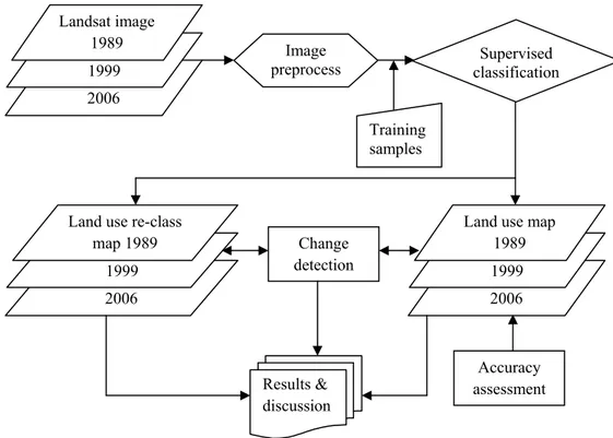
surfaces to use for the future prediction of land use and land covers. The major
landmark processes of the study can be summarized by the flow chart presented as
under (Figure 4). The flow chart of modeling for future land use prediction is placed
in Figure 5 separately.
The methodology employed to predict land uses in the study can be described by the
flow chart given below (Figure 5).
Supervised classification Image preprocess Training samples Landsat image
2006 Landsat image
1999 Landsat image
1989
Land use map 2006 Land use map
1999 Land use map
1989
Accuracy assessment Land use map
2006 Land use map
1999 Land use re-class
map 1989 Change
detection
Results & discussion
Constraints and Factors
3.2. Data
Three Landsat satellite imageries during a period of 17 years were used for the study.
The dates were 1989, 1999 and 2006 and accessed freely from different agencies'
websites8. The date gap of all three acquired imageries was about a week of October
and November. Details of Landsat imageries and characters are given below (Table
7).
Projected Land use 2019
Calibration/ Simulation
Validation
If valid! Original
Land use 2006 Projected Land use 2006 Calibration/
Simulation Land use 1999
Land use 1989
Suitability map
S. N. Satellite Sensor Band Imagery date
Spatial Resolution
(meter)
Path/Row Source
1 Landsat 5 TM 7 1989-10-31 28.5 141/41 Landsat.org
2 Landsat 7 ETM+ 8 1999-11-04 30.0 141/41 USGS
3 Landsat 5 TM 7 2006-10-30 30.0 141/41 USGS
Table 7: Detail characteristics of the Landsat imageries
Landsat images are among the widely used satellite remote sensing data and their
spectral, spatial and temporal resolution made them useful input for mapping and
planning projects (Sadidy, Firouzabadi, Entezari 2009). The other data sets used in
the study were Shuttle Radar Topographic Mission (SRTM) elevation data, digital
topographic map and other layers of Kathmandu valley such as road network, rivers
and water body and designated areas prepared by the Department of Survey, Nepal.
Raw digital images usually contain distortions due to variations in altitude, attitude,
earth curvature and atmospheric refraction, which are corrected by analyzing
well-distributed ground control points (GCPs) present within an image and for which
accurate ground coordinates are available (Kaiser et. al 2008). However, the Landsat
images used in the study were acquired free of distortions from the sources
mentioned above. The spatial references of all processed data sets in the study were
WGS 1984, UTM zone 45 N and Datum D_WGS_1984. The data sets not in WGS
1984 were converted into WGS 1984 mainly digital topographic map and its layers
of Kathmandu valley.
3.3. Software used
The images were processed with various software programs to get required analysis
results. Mentioned below were the software programs used for the study.
• ArcGIS 9.3.1
• Erdas Imagine 9.1
ArcGIS 9.3.1 was used to resample 28.5 meters resolution of image 1989 and 90
meters resolution of SRTM elevation data into 30 meters grid cells and to compose
map of the study area. Nearest neighbor assignment method was used to resample
28.5 meters 1989 image into 30 meters. However to resample 90 meters SRTM
elevation data into 30 meters, bilinear interpolation and cubic convolution were used
since the results were good with these methods. Erdas Imagine 9.1 was used for the
image classifications. Idrisi 15.0 was used for the image differencing,
cross-tabulation and modeling the urban and other land classes change for the current and
future years.
The three classified 1989, 1999 and 2006 maps were exported to ArcGIS 9.3.1 for
map composition and to Idrisi 15 (The Andes Edition) for cross-classification
tabulation and land use and cover change modeling. The cross-classification was
done with re-classified maps i.e. Built up and Non-built up land uses and the
resultant map was obtained for changed and unchanged area of 1989, 1999 and 2006
maps.
3.4. Image classification and accuracy assessment process
Digital image classification is the popular and challenging approach of remotely
sensed image analysis process. In the process pixels in the image are sorted to obtain
meaningful information of the real world as derived in the thematic maps bearing the
information such as land cover type; vegetation type, etc. (Matinfar, 2007).
Although there are different classification systems in existence throughout the world,
they are generally not comparable one to another and also there is no single
internationally accepted land cover classification system (Latham, 2001). Therefore,
determination of land cover classification system is decided considering the purpose
of the study and usually it varies according to different research projects (Tateishi,
The basic principle of multi-spectral classification is that the objects in the earth
surfaces possess different reflectance characteristic in different parts of the
electromagnetic spectrum as digital numbers. Based on this reflectance, the surface
features can be categorized into specified number of classes known as land cover
classes through classification software in terms of new thematic output image. There
are two general classification approaches: supervised and unsupervised. In the
supervised approach the useful information categories are defined and examined for
their spectral separability where in the unsupervised approach, spectrally separable
classes are determined and defined relative to their informational utility to form a
supervised classification scheme (Kaiser et. al. 2008). Supervised classification uses
the independent information from spectral reflectance to define training data for
determining classification categories (Ratanopad and Kainz, 2006). In classification
process, supervised classification has been widely used in remote sensing
applications (Yüksel, Akay, Gundogan, 2008).
The challenges of urban mapping using Landsat imagery include spectral mixing of
diverse land cover components within pixels, spectral confusion with other land
cover features (Guindon, Zhang, Dillabaugh, 2004; Lu, Weng 2006). Therefore, it is
most desirable to set the remote sensing images to obtain good results prior to
classification. For this purpose different image enhancement techniques provided by
the software can be employed. One of spectral enhancement techniques is principal
component analysis. It enhances the spectral discrimination among reflectance of
different features (Kaiser et. al. 2008). Modification of the original bands in digital
image classification has also shown to improve land use land cover classification
accuracy (KC, 2009).
Six land use and cover classes were determined for supervised classification in the
study. The land classes were determined according to the existing practices in the
Kathmandu valley combining with the system adopted by the Department of Survey.
area, and 6) Water. All land areas with agricultural crops were included in
Agricultural land class whereas agricultural lands without crops and exposed areas
were included in Bare soil category. Individual and clusters of building, road
networks, airport, etc were included in Built up. The areas covered with trees were
incorporated in Forest land cover class. Open area was classified for the land areas
with small vegetative ground covers. All kinds of rivers, ponds and lakes were
included in Water land class.
In supervised classification, spectral signatures are collected from specified locations
(training sites) in the image to classify all pixels in the scene by digitizing various
polygons overlaying different land use types (Yüksel, Akay, Gundogan, 2008). For
the classification, training sample should be taken for each of reflection property and
its number varies as per the requirements. Hence, the training samples were collected
accordingly in the spectrally enhanced images for six different land classes as
mentioned above to use in the parametric supervised classification approach. At least
50 samples in an average were taken for each of the land classes to be classified.
Region growing tool was employed for each of training taken to cover maximum
area and the number of pixels per sample. Google Earth, ArcGIS online and digital
topographic maps were used as high resolution references to recognize the pattern of
land use types in the images. A very insignificant amount of areas beneath clouds
were masked stacking in the classification images with the layers of different original
land classes extracted with the help of high resolution references to classify original
land classes.
All three parametric decision rules Maximum likelihood, Mahalanobis distance and
Minimum distance available in the Erdas Imagine 9.1 were employed to classify and
compared the image classification results to choose the best one. Maximum
likelihood algorithm provided good classification results as compared to
Mahalanobis distance and Minimum distance algorithms hence used for further
results of Mahalanobis and Minimum distance classifications are given in the
appendices 1 and 2 respectively.
The accuracy of the result is strongly dependent on the processing procedure,
consisting mainly of geometric correction, image classification and spectral
enhancement (Kaiser et. al. 2008). A common method for accuracy assessment for a
classification image is through the use of an error or confusion matrix and some
important measures, such as overall accuracy, producer's accuracy, and user's
accuracy can be calculated from the error matrix in the classification software.
Ground truth data can be used as training sample data in classification processing or
as correct data in validation step. The information sources of ground truth are field
survey, existing maps, satellite images with better resolution, or any pre-determined
classification system. Since field survey is time consuming and needs much budget,
the latter three sources are usually used (Tateishi, 2002). The testing samples are
used for the establishment of the confusion matrix to assess the classification
accuracy (Long-qian, Li, Lin-shan, 2009). In the study accuracy assessments for all
three classified maps were done with the test samples generated in the software
against high resolution references. The overall test samples generated were 120 for
each of the 1989, 1999 and 2006 classified maps. Google Earth, ESRI online, digital
topographic map and other layers were used as reference due to lack of high
resolution satellite data.
3.5. Land use and cover change modeling and validation
Land-Use & Cover Change (LUCC) modeling is growing rapidly in scientific field.
There are many modeling tools in use but the performance of different modeling
tools is difficult to compare because LUCC models can be fundamentally different in
a variety of ways (Pontius, Chen, 2006). Among the numbers of land use modeling
tools and techniques, the commonly used models are the Cellular Automata Markov
and GEOMOD both available in Idrisi were implemented to predict and compare the
land uses for some further period.
Eastman (2006) defined the terms mostly used in the land use and cover change
modeling, which are MARKOV, STCHOICE, CA_MARKOV, GEOMOD and
VALIDATE. MARKOV analyzes two qualitative land cover images from different
dates and produces a transition matrix, a transition areas matrix, and a set of
conditional probability images. STCHOICE (Stochastic Choice) creates a stochastic
land cover map by evaluating the conditional probabilities that each land cover can
exist at each pixel location against a rectilinear random distribution of probabilities.
CA_MARKOV is a combined cellular automata/Markov change land cover
prediction procedure that adds an element of spatial continuity as well as knowledge
of the likely spatial distribution of transitions to Markov change analysis. GEOMOD
is a land use change simulation model that predicts, forward or backward, the
locations of grid cells that change over time. VALIDATE calculates specialized
Kappa measures that discriminate between errors of quantity and errors of location
between two qualitative maps.
CA_MARKOV can be used to project with any number of land use classes whereas
GEOMOD runs only with two numbers of classes e.g. Built up and Non-built up. A
collection of suitability maps needs to be created as decision rules for simulation
process which can be prepared using Multi-Criteria-Evaluation (MCE). In the
process of creating suitability maps numbers of constraints and factors such as
designated areas, distance from existing urban area, distance from road, distance
from water body, slope, etc must be used that have direct effect in the change of land
uses. The CA_MARKOV uses these suitability maps along with a couple of previous
year's classification maps and Markov transition areas file created using MARKOV
module in the Idrisi. However, GEOMOD uses suitability maps along with beginning
land use map, ending time as well as ending time land classes pixel quantities. The
land use classification map for its reliability to make use of the model predicting
further year's land use and land cover.
According to Pontius, Chen (2006), it is desirable to validate the accuracy of the
prediction after the creation of simulated map of the ending time. Although there are
different ways of validating the simulated map output, the most used one is
VALIDATE module technique in Idrisi. The VALIDATE module examines the
agreement between two maps that show the same categorical variable i.e. comparing
a pair of true ending time map versus simulated ending time map. In the comparison,
the true ending time map is referred as "reference map" and the simulated map as
"comparison map". The validation results offer a comprehensive statistical analysis
that answers simultaneously the two important questions: 1) "How well do a pair of
maps agree in terms of the quantity of cells in each category? and 2) "How well do a
pair of maps agree in terms of the location of cells in each category?"
3.6. Discussion
This chapter describes different data sets acquisition procedure used in the study and
review of different approaches of image classification and land cover change
modeling as the basis for selection of the preferred techniques. Three Landsat images
during 1989 to 2006 were undergone with preprocessing from resample of 1989
image to final selection of best resulted image enhancement technique and
classification algorithm available in the software for image classification. Principle
component analysis spectral image enhancement technique and maximum likelihood
algorithm were used for the classification. Maximum likelihood algorithm provided
good classification results as compared to Mahalanobis distance and Minimum
distance algorithms and used for further processing. CA_MARKOV and GEOMOD
4. RESULTS
4.1. Introduction
The main aims of the study were to focus on the urban change analysis during the
1989 to 2006 period and to know the trend of urban growth in the further years by
projecting urban land class using CA_MARKOV and GEOMOD available in Idrisi.
All the results derived from image classification, change analysis, land use and cover
change model calibration, implementation and validation are presented and discussed
in this chapter.
4.2. Image classification
4.2.1. Preprocessing
The information for each specific wavelength range stored as a separate image is
called a band which is similar to a black and white digital photograph. It is up to the
analyst to combine the images from the different wavelengths to create a color image
(Horning, 2009). So, after the entry of the images into the software program,
composite layers were made by stacking all band layers of each three year's images
(Figure 6). Composite layer of all three images were again subset into the study area.
The resolution of 1989 image was 28.5 meters (seems smaller than other images in
figure 6) which was made 30 meters by resample technique after subset of study
Figure 6: Composite bands of 1989, 1999 and 2006 images showing study area in yellow square [True color]
Principal component analysis was implemented for all three images (Figure 7). It
enabled the spectral enhancement, especially for built up and water which had
similar reflectance, of the images to easily distinguish for extracting the land classes
of the study area. The three spectrally enhanced images were used for the
classification and re-classification of the land use and land cover. The training
samples were then taken for each of the 1989, 1999 and 2006 enhanced images. An
example to show training samples taken in the images is presented in the following
Figure 7: Spectrally enhanced 1989, 1999 and 2006 images of the study area [Band: 3, 2, 1]
Presented below is an illustrative example for showing training samples taken for the
classification of 1989, 1999 and 2006 images (Figure 8).
Training samples
4.2.2. Image classification
The 1989, 1999, and 2006 images were classified into six classes (Figure 9). The
overall total area of the land use classes of the study area was 88491 hectare. The
maps and the detail statistics of the classification results are given below (Table 9).
Figure 9: Land use land cover classification maps of Kathmandu valley
The land use classes and the areas derived from the classification of 1989, 1999 and
2006 images are given in the following table 8. The area statistics of the land uses
and land covers could better be quantified if interpreted with visual support than
ID Land use class Area in hectare 1989 1999 2006
1 Agriculture 13350 12944 14420
2 Bare soil 17434 23742 21140
3 Built up 2454 4366 5732
4 Forest 28044 28366 31509
5 Open area 26266 18680 15267
6 Water 943 393 423
Total 88491 88491 88491
Table 8: Land use class types of class areas
The bar chart below visually quantifies the six land uses in each date and can be
interpreted transitions between different land use classes (Figure 10). The Built up
area had increased and water class decreased by more than two folds during the study
period. The chart shows that the Open area land class was also the most decreased
class followed by Bare soil land class. The rest of the land uses had not changed
significantly. 0 10000 20000 30000 40000 50000 60000 70000 80000 90000
1989 1999 2006
13350 12944 14420
17434 23742 21140
2454 4366 5732
28044
28366 31509
26266 18680 15267
943 393 423
Area in hectare Year Water
Open area
Forest
Built up
Bare soil
Agriculture
4.2.3. Accuracy assessment
The result of classifications of 1989, 1999 and 2006 images were evaluated through
the accuracy assessment process. Accuracy assessment process started with taking
number of test samples in an image used for the classification and verifying the
samples with high resolution image as a reference. Figure 11 below shows an
illustrative example of test samples taken in an image for accuracy assessment. The
yellow colored samples were converted into white color after the verification of land
classes with the help of reference image (Figure 11).
Test samples
Figure 11: An example for test samples taken in an image
The indices used for the evaluation were overall accuracy, overall Kappa (κ) as well as producer's and user's accuracy for individual land classes. The results are presented below (Table 9).
1989 1999 2006 Overall classification accuracy (%) 86.67 88.33 89.17
Overall Kappa (κ) statistics 0.8196 0.8351 0.8576
The results show that the achieved overall classification accuracies were 86.67%,
88.33% and 89.17% and overall Kappa (κ) statistics were 0.8196, 0.8351 and 0.8576 respectively for the classification of 1989, 1999 and 2006 images. The producer's and User's accuracy for individual land classes were as follows (Table 10).
Class name 1989 (%) 1999 (%) 2006 (%)
Producer's User's Producer's User's Producer's User's
Agriculture 85.00 80.95 100.00 53. 33 81.25 68.42
Bare soil 75.00 94.74 92.31 100.00 93.55 100.00
Built up 83.33 100.00 100.00 100.00 100.00 100.00
Forest 93.75 95. 74 84.00 95.45 90.70 95.12
Open area 86.36 70.37 85.71 78.26 84.21 76.19
Water --- --- --- --- 100.00 100.00
Table 10: Producer's and User's accuracy for individual land classes
The ranges attained for producer's accuracy were 75% - 93.75%, 84% - 100% and
81.25% - 100% whereas user's accuracy were 70.37% - 100%, 53.33% -100% and
68.42% -100% respectively for the classification of 1989, 1999 and 2006 images. It
was apparent from the results that the lowest producer's and user's accuracies could
not be attained for the same land classes during the classification years. However,
higher producer's and user's accuracies could mostly for Built up land class. This
might be because of the focus of the study more to the urban change analysis.
Land use and land cover reclassification
Since the study is focused mainly on urban land class change, the land use and land
cover maps were re-classified into Built up and Non-built up land classes (Figure 12)
and mentioned below were the results and statistics of the image re-classification
Figure 12: Land use re-classification maps of Kathmandu valley
The land classes and the areas derived from the re-classification of 1989, 1999 and
2006 images are given in the following table 11. The result statistics in table below
have been explained with the following bar chart.
ID Land use class Area in hectare 1989 1999 2006
1 Built up 2454 4366 5732
2 Non-built up 86037 84125 82759
Total 88491 88491 88491
The bar chart below (Figure 13) shows visually the quantities of Built up and
Non-built up land class changes. The statistics on chart explain that Built up areas was
increased more than 2 times during the study period.
0 20000 40000 60000 80000 100000
1989 1999 2006
2454 4366 5732
86037 84125 82759
Area in hectare Year
Built up
Non‐built up
Figure 13: Bar chart land use quantization in 1989, 1999 and 2006
4.2.4. Change analysis
The changes in area in hectare and percentage of all the land use classes and land use
re-classes are presented below (Table 12, 13).
ID Land use
Area change in hectare Area change in %
1989-1999 1999-2006 1989-2006 1989-1999 1999-2006 1989-2006
1 Agriculture -406 +1476 +1070 -3.0 +11.0 +8.0
2 Bare soil +6308 -2602 +3706 +36.0 -11.0 +21.0
3 Built up +1912 +1366 +3278 +78.0 +31.0 +134.0
4 Forest +322 +3143 +3465 +1.0 +11.0 +12.0
5 Open area -7586 -3413 -10999 -29.0 -18.0 -42.0
6 Water -550 +30 -520 -58.0 +8.0 -55.0
The table 13 shows that the areas of Open area and Water land classes decreased
significantly. The Built up area has been increased by 134% during the study period.
ID Land use
Area change in hectare Area change in %
1989-1999
1999-2006
1989-2006
1989-1999
1999-2006
1989-2006
1 Built up +1912 +1366 +1366 +78.0 +31.0 +134.0
2 Non-built up -1912 -1366 -1366 -2.0 -2.0 -4.0
Table 13: Area change in hectare and percentage of land re-classes
The table 13 shows that a significant amount of the Built up area has been increased
during the study period.
The cross classification map below (Figure 14) shows the quantity of area change
between the Built up and Non-built up land use classes. The map shows that during
the 1989 to 2006 period 2454 hectare of Built up and 82759 hectare of Non-built up
areas remained unchanged. 1912 and 3278 hectares of Non-built up area had been
Figure 14: Cross classification of Built up and Non-built up land classes
4.3. Land use and cover change modeling
4.3.1. Model calibration
The modeling process involved number of complex steps. One of these was to create
suitability map that could be used as decision rules to predict future land uses and
land covers. The low to high suitability range (0 to 255 or 0 to 100) is the decision
rule that restricts or allows particular land uses to grow up and/or transform into each
other. Two methodologies were employed for creating the suitability maps and their
collection. They were explained as "First Methodology" and "Second Methodology"
A. First Methodology
In the first method of creating suitability map, numbers of factors and constraints
have been combined. The factors and constraints are the criteria for urban to grow
and developed from the Boolean (logical) images which have values 0 = unsuitable,
and 1 = suitable.
• Constraints:
Constraints are the Boolean conditions which limit the alternatives under
consideration (Eastman, 2006). The examples of constraint are the existing built up
area, protected areas like forest and wildlife reserve and water bodies, etc. where
expansion of urban is restricted. In this case, Forest and Open areas were set as
constraints because they have been considered as public properties. The designated
areas in the Kathmandu valley i.e. Shivapuri Watershed and Wildlife Reserve and
Gokarna and Nagarjun Reserve Forests were also included inside the Forest and
Open areas. The Built up and Forest and Open areas constraints were derived from
the land use classification map of 1999 and the Water constraint is derived from the
digital layers of rivers and water bodies from Department of Survey. The following
constraints images were derived from the processes as mentioned above (Figure 15).
Forest and Open areas Built up
Water
Figure 15: Constraints used to create suitability maps for urban growth
(0-unsuitable; 1-suitable)
The Boolean condition is only possible when all the criteria of interest have only 0 =
unsuitable, and 1 = suitable values. However, there are some criteria which have low
to highest preference on suitability rather than 0 = unsuitable, and 1 = suitable. So
every image with Boolean condition for factors was standardized into probability
range of suitability between 0 and 255 for urban growth.
• Factors:
Factor is continuous gauge of suitability measured in 0-255 scale. It enhances or
consideration (Eastman, 2006). For example, nearness to existing built up, roads,
certain land uses and relatively flat areas etc. have high level of suitability to develop
urban areas and suitability decreases as the distance decreases and slope increases.
However the degree of suitability decreases as the nearness to water body increases.
These principles generally should be based on the government policy formulated
according to environmental and socio-economic consideration. The development of
urban areas should mostly be preferable to underutilized places but these kinds of
areas are rarely available in the cities. So, agricultural areas having relatively flat
slopes are being extensively utilized nowadays for the urban development. It is also
supposed that the urban development takes place closest to existing road networks
and developed unoccupied areas. Preference level lowered down as their distances
increase due to cost effectiveness. Nearness to water body should also be avoided for
the urban development. Considering these general principles the factors with
Boolean condition were standardized into "fuzzy" rule, i.e. suitability of contiguous
range of 0 = least suitable to 255 = most suitable using Multi Criteria Evaluation
(MCE) in Idrisi.
The fuzzy module available in Idrisi is characterized to standardization of Boolean
factors into entire range of criteria of "none" to "full" possibilities to transform into
either a binary (0 and 1) or a byte (0 to 255) output data format without sharp
boundaries as 0 = lowest to 255 = highest suitability for growth where the latter
output data format option is recommended because the MCE module has been
optimized for using a 0-255 level of standardization (Eastman, 2006). The Idrisi
supported monotonically increasing, monotonically decreasing, symmetric, and
asymmetric variants and the fuzzy set membership functions: sigmoid, j-shaped, and
linear (Eastman, 2006), are available to utilize as control points for the set
membership function. The selection of these variants and range of control points
fully depends on the analyst familiarity to the study area. The perfectness of selection
can be measured in the model validation stage. These criteria were set according to
Factor Membership function/variant Control point Explanation Distance from built up
Linear/decreasing 0 - 6508 0-6508 is the minimum and
maximum distance values of the
built up area in 1999, linear
decreasing criteria was set since
suitability decreases as distance to
built up increases
Distance
from the
roads
Linear/decreasing 0-7946 Linear decreasing criteria was set
since suitability decreases as
distance to from roads increases
Slopes Sigmoid/decreasing 0-25
degree
Slopes between 0 to 25 degree are
considered most suitable
Distance
from water
bodies
Linear/increasing
30-10061
It was assumed that the areas within
30 meter from the water bodies
should have low suitability and
above this distance suitability
increases
Table 14: Criteria to standardize fuzzy module
The land use factor was not considered in the table because it was created by
assigning the value for Agriculture and Bare soil land classes as highest suitability
and existing built up as the lowest suitability with Edit/ASSAIGN module in Idrisi.
The following factor images were derived from the processes as described above in a
Built up Land use
Roads Slopes
Water
Figure 16: Factor maps showing range of suitability to urban growth
Different factors have different importance affecting the urban growth while creating
the overall suitability. Therefore, the weight to each of the factor image was assigned
according its importance. Although, variety of techniques exist for the development
the information down into simple pair wise comparisons into two criteria considered
at a time can produce a more robust set of criteria weights which can be available as
Analytical Hierarchy Process (AHP) by Saaty (1977) in Idrisi (Eastman, 2006). The
process requires weighting factors rate from extremely "less important" (1/9) to
"more important" (9). Consistency ratio (CR) is calculated as the AHP ratings are
filled out to identify the inconsistencies in the pair wise comparison ratings.
According to Eastman (2006), Saaty indicates that CR greater than 0.1 should be
re-evaluated. The assignment of rating needs analyst intuition and repetition unless the
consistency is acceptable as shown below (Figure 17).
Figure 17: Analytical Hierarchy Process (AHP) ratings and Consistency ratio
The AHP weights derived from the pair wise comparison matrix to be assigned each
of the factors are discussed in the table 15 below (Table 15).
S. N. Factors Weight
1 Built up 0.0685
2 Land use 0.1220
3 Road 0.5212
4 Slope 0.1759
5 Water 0.1125
Once the constraints and factors were developed and factors weights were derived,
all the information was aggregated using Weighted Linear Combination (WLC)
available in MCE module in Idrisi. The WLC multiplies each factor images by its
weights and sums the results which will have the same range of values as
standardized factor images used. The result is then multiplied by each of the
constraints to mask out unsuitable areas as the resultant suitability map.
The resultant suitability map used for projecting the urban growth was as under
denoted as "Highly suitable" (Figure 18). The suitability map was prepared using
numbers of constraints and factors as mentioned above. The next map denoted as
"Highly unsuitable" was the inverse of resultant suitability map to be used together in
a group created by Collection Editor menu in Idrisi.
Highly suitable Highly unsuitable
Figure 18: Suitability maps showing high to low range of suitability to urban growth
The next step was to use MARKOV module to create a transition probability matrix,
a transition areas matrix and a set of conditional probability images. These were
created using 1989 and 1999 land use maps. The conditional probability images was
the input in STCHOICE as a group file where the transition area matrix was one of
inputs necessary to run the CA_MARKOV module along with basis land cover
image and transition suitability image collection created above. CA_MARKOV uses

![Figure 2: Kathmandu valley in 3D perspective [Band: 3, 2, 1]](https://thumb-eu.123doks.com/thumbv2/123dok_br/15755615.638803/16.892.202.729.185.469/figure-kathmandu-valley-d-perspective-band.webp)


![Figure 6: Composite bands of 1989, 1999 and 2006 images showing study area in yellow square [True color]](https://thumb-eu.123doks.com/thumbv2/123dok_br/15755615.638803/37.892.181.747.127.618/figure-composite-bands-images-showing-study-yellow-square.webp)


