INTRODUCTION
A diallel is a mating system that involves all pos-sible crosses among a group of parents. This genetic design is used to study polygenic systems that determine quantita-tive traits. Depending on the nature of the parents, individu-als from an open pollinated variety or an F2 generation, or selected open pollinated varieties or line cultivars, inferences based on diallel results are useful in planning base popula-tions for intra and/or interpopulation improvement or par-ents for hybridization. The partial diallel is one of many variations of the diallel (Griffing, 1956; Kempthorne and Curnow, 1961; Gardner and Eberhart, 1966) and consists of crosses among two parent groups. This mating system, also called experiment II, design II and factorial design, was proposed by Comstock and Robinson (1948, 1952). It is adequate when there are distinct groups of populations, for example one group of dent inbred lines and the other of flint inbred lines, derived from a reciprocal recurrent selection pro-gram, and the breeder is not interested in evaluating the crosses between parents of the same group. The two parent groups can involve adapted or commercial populations and exotic germplasm or plant introductions, for example, dwarf cashew tree and normal clones, small and large seeded cultivated com-mon beans, acom-mong many others. As generally the parents are open-pollinated populations or pure lines defined by the breeder, there is no base population for inferences. The infer-ences must be established in relation to the set of parents.
Jinks and Hayman (1953) and Hayman (1954, 1958)
presented methods for diallel analysis, with a firm and re-fined theoretical basis, using data from parents and their F1 progeny or parents, F1 and F2 generations. These meth-ods have been used ever since (Jinks, 1954; Dickson, 1967; Chung and Stevenson, 1973; Kornegay and Temple, 1986; Nishimura and Hamamura, 1993), although the method-ologies proposed by Griffing (1956) and Gardner and Eberhart (1966) are the most frequently employed. Limi-tations of these methods are discussed by Gilbert (1958), Nassar (1965), Coughtrey and Mather (1970), and Sokol and Baker (1977).
As Hayman’s proposals (1954, 1958) are not valid for partial diallels, a separate theory is required. The theory and analysis of partial diallel crosses presented are a gen-eralization of the methodology of Hayman (1954). If gene frequencies are the same for the two parent groups, results are equal to those presented by Hayman.
METHODOLOGY
General theoretical considerations
Consider a polygenic system with k genes con-trolling a quantitative trait in a diploid species and the following conditions: a) Mendelian inheritance; b) ab-sence of reciprocal effects; c) abab-sence of non-allelic in-teraction; d) no multiple allelism; e) no correlation in the distribution of non-allelic genes in the parents, and f) homozygous parents. If N parents (N ≥ 6) are divided into two groups, one with n and the other with n’ parents (n + n’ = N, n and n’ ≥ 3), three polygenic systems are defined: one related to the group with n parents, one as-sociated to n’ parents and the last related to N parents. Let pr be the genotypic value of the rth parent of the n
THEORY AND ANALYSIS OF PARTIAL DIALLEL CROSSES
José Marcelo Soriano Viana1, Cosme Damião Cruz1 and Antonio Américo Cardoso2
A
BSTRACTThis study presents theory and analysis of partial diallel crosses based on Hayman’s methods. This genetic design consists of crosses among two parental groups. It should be used when there are two groups of parents, for example, dent and flint maize inbred lines, and the breeder is not interested in the assessment of crosses between parents of the same group. Analyses are
carried out using data from the parents and their F1 hybrids allowing a detailed characterization of the polygenic systems
under study and the choice of parents for hybridization. Diallel analysis allows the estimation of genetic and non-genetic components of variation and genetic parameters and to assess the following: genetic variability in each group; genotypic differences between parents of distinct groups; if a parent has a common or a rare genotype in the group to which it does not belong; if there is dominance; if dominant genes increase or decrease trait expression (direction of dominance); average degree of dominance in each group; the relative importance of mean effects of genes and dominance in determining a trait; if, in each group, the allelic genes have the same frequency; if genes are equally frequent in the two groups; the group with the greatest frequency of favorable genes; the group in which dominant genes are most frequent; the relative number of dominant and recessive genes in each parent; if a parent has a common or a rare genotype in the group to which it belongs, and the genotypic differences between parents of the same group. An example with common bean varieties is considered.
1Departamento de Biologia Geral and 2Departamento de Fitotecnia,
Universidade Federal de Viçosa, 36570-000 Viçosa, MG, Brasil. Send cor-respondence to J.M.S.V.
a
a a a
a
a
a a
a a a a a
parental group and ps the genotypic value of the sth par-ent of the n’ parpar-ental group. Thus:
pr = m + Σ da θra (r = 1, …, n)
ps = m + Σ da θsa (s = 1, …, n’), m = Σ ma
If pt is the genotypic value of the tth parental in the N parental group, then:
pt = m + Σ da θta (t = 1, …, N)
For all loci in the polygenic system under study, the parameter da is the difference between the genotypic value of the homozygote of largest expression and the genotypic mean of the homozygotes (ma). The θ variable assumes the value -1 or 1 depending on if the parent is homozygous for a gene which diminishes or increases trait expression, re-spectively. If ua and va are frequencies of alleles that in-crease and reduce trait expression, respectively, the follow-ing expectation and variance apply to the n parental group:
E(θra) = ua - va = wa
V(θra) = 1 - w2
In relation to the n’ parental group:
E(θsa) = u’ - v’ = w’
V(θsa) = 1 - w’2
In the group formed by N parents:
E(θta) = ua - va = wa = pwa + qw’,
with ua = pua + qu’ ,va = pva + qv’, p = n / N, and q = n’ / N, and
V(θta) = 1 - w2 = 1 - p2w2 - q2w’2 - 2pqw w’ = 4uava
Genotypic mean of the n parental group is:
E(pr) = mL0 = m + Σ da wa
Genotypic mean of the n’ parental group is:
E(ps) = m’ = m + Σ da w’
Genotypic mean of N parents is:
E(pt) = mL0 = m + Σ da wa = pmL0 + qm’
Diallel analysis of parents and their F1 hybrids
The genotypic mean of the hybrid derived from the k
a = 1
L0 a
k
a = 1
L0 k
a = 1 k
a = 1
k
a = 1
k
a = 1
k
a = 1
rth and sth parents is:
frs = m + Σ [da (θra + θsa) + ha (1 - θraθsa)] =
= (pr + ps) + Σ ha (1 - θraθsa),
with Σ ha (1 - θraθsa) = hrs being the specific heterosis of the rth and sth parents. The parameter ha is the difference between the genotypic value of the heterozygote and ma.
The genotypic mean of the hybrids from the rth parent or mean of the rth array is:
E(frs) = fr = m + Σ [da (θra + w’) + ha (1 - w’θra)] =
= (pr + m’ ) + Σ ha (1 - w’θra),
where Σ ha (1 - w’θra) = hr is the varietal heterosis of the rth parent.
The genotypic mean of the hybrids from the sth parent or mean of the sth array is:
E(frs) = fs = m + Σ [da (θsa + wa) + ha (1 - waθsa)] =
= (ps + mL0) + Σ ha (1 - waθsa),
where Σ ha (1 - waθsa) = hs is the varietal heterosis of the sth parent.
The genotypic mean of the F1 hybrids is:
E(frs) = E(fr) = E(fs) = mL1 = m + Σ [da (wa + w’) +
+ ha (1 - waw’)] = (mL0 + m’ ) + Σ ha (1 - waw’),
where Σ ha (1 - waw’) = h is the average heterosis.
Thus,
mL0 - m’ = Σ 2da (ua - u’)
mL1 - (mL0 + m’ ) = h
In the presence of dominance, specific heterosis of the rth and sth parents is nil if the parents have the same genotype (θraθsa = 1, for every a) and greatest when the parents are carriers of distinct alleles at the k loci (θraθsa = -1, for every a). Varietal heterosis of a parent is least when it carries the most frequent genes in the group of parents to which it does not belong and greatest if it is the carrier of the least frequent genes. If deviations due to dominance
k
a = 1 1 2
k
a = 1 1 2 1
2
k
a = 1
a a r fixed a L0 a k
a = 1
1 2
k
a = 1
1 2
k
a = 1 1
2
a
a a
k
a = 1 a
1 2 1
2 L0
k
a = 1
L0 L0 a 1 2 k
a = 1
1 2
k
a = 1
1 2 1 2 s fixed k
a = 1
k
a = 1 1 2 k
are of the same magnitude and the varietal heterosis in a group is constant, the allelic genes in the other parental group have the same frequency (wa or w’ equal to zero, for every a). Since (1 - wa w’) ≥ 0, if h > 0, positive unidirec-tional dominance is established. In other words, the devia-tions due to dominance should be predominantly positive. If h = 0 and there is dominance, positive and negative de-viations are present (bi-directional dominance). Dominance is negatively unidirectional when h < 0.
If mL0 - m’ is greater than zero, there is evidence that genes which increase trait expression are more fre-quent in the n parental group. If this difference is nega-tive, genes which increase trait expression should be more frequent in the n’ parental group. When the difference is nil, genes are equally frequent in the two parental groups (wa = w’, for every a) or, alternatively, some genes which increase trait expression are more frequent in one group of parents, while others are more frequent in the other group.
Genetic components of variation
Analysis of the diallel table allows the definition of the following second degree statistics:
(1) Variance of the genotypic means of the n parents
V0L0(1) = V(pr) = Σ d2 (1 - w2) = 4 Σ ua va d2 = D(1)
(2) Variance of the genotypic means of the n’ parents
V0L0(2) = V(ps) = Σ d2 (1 - w’2) = 4 Σ u’ v’ d2 = D(2)
(3) Variance of the genotypic means of the N parents
V0L0 = V(pt) = Σ d2 (1 - w2) = D = p2D(1) + q2D(2) + 2pqD(3),
D(3) = Σ d2 (1 - wa - w’)
(4) Covariance between genotypic mean of rth parent hy-brid and the mean of the nonrecurrent parent (covariance in the rth array)
W01(r)L01 = Wr = Cov(frs, ps) = D(2) - Fr
Fr = 2 Σ dahaθra (1 - w’2)
(5) Variance of the genotypic means of the rth parent hy-brids (variance in the rth array)
V1(r)L1 = Vr = V(frs) = D(2) - Fr + H1(2),
H1(2) = Σ h2 (1 - w’2) = 4 Σ u’v’h2
(6) Covariance in the sth array
W01(s)L01 = Ws = Cov(frs, pr) = D(1) - Fs,
Fs = 2 Σ dahaθsa (1 - w2)
(7) Variance in the sth array
V1(s)L1 = Vs = V(frs) = D(1) - Fs + H1(1),
H1(1) = Σ h2 (1 - w2) = 4 Σ uavah2
(8) Covariance between genotypic mean of rth parent hy-brid and the mean of the nonrecurrent parent array
W01(r)L1 = Cov(frs, fs) = D(2) - Fr - F(1) + H1(2) - H2r,
F(1) = E(Fr) = 2 Σ dahawa (1 - w’2) = 8 Σ u’v’ (ua - va)daha
H2r = Σ h2 (1 - waθra) (1 - w’2)
(9) Covariance between genotypic mean of sth parent hy-brid and the mean of the nonrecurrent parent array
W01(s)L1 = Cov(frs, fr) = D(1) - Fs - F(2) + H1(1) - H2s,
F(2) = E(Fs) = 2 Σ dahaw’ (1 - w2) = 8 Σ uava (u’ - v’)daha
H2s = Σ h2 (1 - w’θsa) (1 - w2)
(10) Variance of the genotypic means of the F1 hybrids
V(frs) = VF1 = [D(1) + D(2) - F(1) - F(2) + H1(1) + H1(2) - H2],
H2 = E(H2r) = E(H2s) = Σ h2 (1 - w2) (1 - w’2) =
= 16 Σ uava u’v’h2
Analysis of the magnitude and significance of the additive components D(1) and D(2) allows establishment of several inferences about genetic variability of each paren-tal group. If the additive component of a group is nil, the parents have the same genotype (w2 = 1 or w’2 = 1, for every a) and, therefore, there is no genetic variability. When nonfixed genes are involved, the parents have distinct geno-types and the additive component is different from zero. Its value is largest when alleles are equally frequent.
The following differences are also useful:
D(1) - D(2) = Σ d2 (w’2 - w2) and 2D(3) - D(1) - D(2) = = Σ d2 (w
a - w’)2 a a a L0 r fixed 1
4 1 8 1 8 1 4 1 4 k
a = 1 a a a
k
a = 1
k
a = 1 a a
1 4
k
a = 1 a a a
a a a k
a = 1
k
a = 1 a a a
a a
k
a = 1 k
a = 1
a a
k
a = 1 a
a a
k
a = 1
k
a = 1 a a a
k
a = 1 a a
a a
k
a = 1
1 2 1 4 k
a = 1 a
r fixed
,
1
4 1 4 1 4
r fixed k
a = 1 a a a a
k
a = 1 a
1 2 k
a = 1
s fixed 1 4 a s fixed 1
4 1 4 1 4 k
a = 1 a a a
k
a = 1
1
4 1 8 1 8 1 4
s fixed
a a
k
a = 1
k
a = 1 a a
k
a = 1 a a a
1 4
If the differences are nil, the genes are equally fre-quent in the two parental groups. If not, it can be con-cluded that the genes do not have the same frequency in the two groups. When D(1) - D(2) < 0, the n’ parental group is more variable. If genetic variation is greater in the n parental group, then D(1) - D(2) > 0.
The F component of a parent can be negative, nil or positive. When negative, it indicates that the parent has more recessive than dominant genes (haθa < 0). If positive, the parent has more dominant genes (haθa > 0). If there is no dominance, F values of the parents are nil. When domi-nance exists, F = 0 indicates that the parent carries ap-proximately the same number of dominant and recessive genes. For any parental group, the F value of one parent is directly proportional to the number of dominant genes it carries that are not fixed in the other group of parents. Therefore, the F value of a parent is largest when it carries all the dominant genes that are not fixed in the other group. The average F value of a parental group indicates the fre-quencies of dominant and recessive allelic genes. When it is positive, it indicates that dominant genes are more fre-quent than recessive alleles in that group (hawa > 0 or haw’ > 0). If recessive genes are more frequent in the group, its value is negative (hawa < 0 or haw’ < 0). If there is dominance and the average F value is nil, the alleles are equally frequent.
Given the presence of genetic variability among parents in a group, the H1 component of the group will be nil in the absence of dominance and positive in the presence of dominance. The difference H1(1) - H1(2) pro-vides the same information as D(1) - D(2). If there is ge-netic variability in the two parental groups, components H2r, H2s and H2 will be positive in the presence of domi-nance and nil in its absence. Absence of variability in a parental group makes components F and H2 of parents from the other group, and their respective average val-ues, to be nil. Dominance components H1(1), H1(2) and H2 have the same magnitude when allelic genes have the same frequency in the two parent groups (ua = u’ = 1/2, for every a).
In the presence of dominance, the relative mag-nitude of H2 components of parents in a group supplies important information. The H2 component of a parent is largest when it carries the least frequent genes of the group to which it belongs (waθra or w’ θsa < 0, for every a), and smallest when it carries the most frequent genes (waθra or w’θsa > 0, for every a). Generally, the value of the H2 component of a parent is inversely proportional to the concentration of the most frequent genes of its group, that are nonfixed in the other group. The differ-ence between H2 components of two parents from the same group can be nil, if the parents have the same geno-type or if the most frequent genes in the parents are different. If all H2 components of parents in a group have the same magnitude, allelic genes are equally fre-quent in the group.
Genetic parameters
Average values of uv and u’v’
If ua = u, H2/4H1(2) = uv. If u’ = u’, then H2/4H1(1) = u’v’. If ua = u’ = u, the two ratios are equal to uv. Thus H2/ 4H1(2) and H2/4H1(1) express the average value of the al-lelic frequency products in groups with n and n’ parents, respectively.
Average degree of dominance (h/d)
If ha = h and da = d, then H1(1)/D(1) and H1(2)/D(2) are equal to h/d. Therefore, H1(1)/D(1) and H1(2)/D(2) ex-press the average degree of dominance in the polygenic systems defined by the n and n’ parental groups, respec-tively.
Proportion between dominant and recessive genes in parents of the same group
Following Hayman’s approach, it can be demon-strated that the ratios
4D(2) H1(2) + F(1) 4D(1) H1(1) + F(2) 4D(2) H1(2) - F(1) 4D(1) H1(1) - F(2)
reflect the average value of the proportion between the number of dominant and recessive genes in the n and n’ parental groups, respectively. A ratio close to zero indi-cates that parents in the group have few dominant genes and many recessive ones. A ratio near one indicates that parents in the group have the same number of dominant and recessive genes. A ratio larger than one indicates that parents in the group have many dominant genes and few recessive ones.
Direction of dominance
Defining k+ and k- as the number of dominant genes which increase and decrease trait expression, respectively, average heterosis can be expressed in the following way:
h = Σ ha (1 - wa w’) - Σ ha (1 - wa w’), k+ + k-≤ k,
If ha = h, da = d, wa = w and w’ = w’, then:
h2 D
(1)D(2) / H2D2 =
If ha = h, da = d and wa = w’ = w, then h2/H2 = (k+ -k-)2/k. Therefore, if dominance exists in the polygenic sys-tem under study, but the above ratio is nil, the number of a
a
a
a
a
a
a
a and
a a
k+
a = 1
k-a = 1
a
k (3)
dominant genes with a positive effect is the same as the number of dominant genes with a negative effect. In other words, dominance is bi-directional. If the ratio is positive, the numbers of dominant genes which increase and de-crease trait expression are unequal, that is, dominance is predominantly unidirectional.
The relationship between variance and covariance in the arrays
Considering the additive-dominant model the dif-ferences Wr - Vr = (1/4)(D(2) - H1(2)) and Ws - Vs = (1/4)(D(1) - H1(1)) are constant for every r and s. Thus, the coeffi-cients of the regressions of Wr as a function of Vr (Wr = β0 + β1Vr) and Ws as a function of Vs (Ws = β0 + β1Vs) are equal to 1. Intercepts of the regressions of Wr on Vr as well as Ws on Vs are, respectively:
β0 = E(Wr - Vr) = (D(2) - H1(2))
β0 = E(Ws - Vs) = (D(1) - H1(1))
Similarly to Hayman (1954), it can be shown that (Wr, Vr) and (Ws, Vs) values occur on the straight line de-limited by the parabola W2 = V
0L0(2)Vr and W2 = V0L0(1)Vs, respectively. If analysis of variance of the differences Wt -Vt indicates that Wr - Vr and Ws - Vs are constants and/or, if the regression analyses of Wr on Vr and Ws on Vs show that β1 = 1, the additive-dominant model adequately de-scribes the observed results. When, β1≠ 1, the additive-dominant model is inadequate. Hayman (1954, 1958) and Mather and Jinks (1974) presented detailed discussions about the causes of inadequacy of the additive-dominant model, including the presence of extranuclear gene effects, non-allelic interaction, multiple allelism, correlation in the distribution of non-allelic genes and heterozygosis in the parents. Hayman (1954, 1958) also discussed how to pro-ceed with diallel analysis when one or more of the addi-tive-dominant genetic model restrictions are not fulfilled. Absence of a relationship between Wr and Vr and between Ws and Vs (β1 = 0) indicates the absence of domi-nance in the polygenic system under study, since, when ha = 0, Wr = (1/2)D(2), Vr = (1/4)D(2), Ws = (1/2)D(1) and Vs = (1/4)D(1). Thus, when W is plotted against V for each group, all points occur at the ((1/2)D, (1/4)D) position. When the additive-dominant model is adequate, the constant of the regression of Wr on Vr indicates the average degree of dominance in the polygenic system defined by the n’ pa-rental group. The intercept of the regression of Ws on Vs expresses the average degree of dominance in the poly-genic system defined by the n parental group. If β0 < 0, there is evidence of overdominance. When β0 = 0, there is complete dominance. Partial dominance exists when β0 > 0. If the genes are equally frequent in the two parental groups, then:
D(1) = D(2) = D(3) = D
F(1) = F(2) = F
H1(1) = H1(2) = H1
Wr - Vr = Ws - Vs = Wt - Vt = (D - H1)
Thus, the coefficient of the regression of Wt on Vt (Wt = β0 + β1Vt) is equal to one, and the intercept is (1/ 4)(D - H1), if the additive-dominant genetic model is ad-equate. The straight line is delimited by the parabola W2 = DVt.
The relationship between the sum of the variance and covariance in the arrays and the genotypic value of the common parent
It has already been demonstrated that variance and covariance in an array are smallest when the common par-ent is a carrier of dominant genes and largest when it is a carrier of recessive genes. Thus, the relationship between the genotypic value of the common parent and the sum between the variance and covariance in the parent array (pr = β0 + β1(Wr + Vr) or ps = β0 + β1(Ws + Vs)) defines the presence and direction of dominance. The regression co-efficient of pr on Wr + Vr is:
- Σ d2h
a (1 - w2) (1 - w’2) Σ d2 h2 (1 - w2) (1 - w’2)2
The coefficient of the regression of ps as a function of Ws + Vs is:
- Σ d2h
a (1 - w2) (1 - w’2) Σ d2 h2 (1 - w2)2 (1 - w’2)
The existence of a relationship between the ge-notypic value of the common parent and the sum between variance and covariance in its array indicates the pres-ence of unidirectional dominance. If the regression coef-ficient is positive, deviations due to dominance are pre-dominantly negative, contributing to a decrease in trait expression. If the coefficient is negative, the deviations of dominance contribute, exclusively or mostly, to an in-crease in trait expression. If there is no dominance, the graphic points of pr over Wr + Vr and ps over Ws + Vs are (pr, (3/4)D(2)) and (Ps, (3/4)D(1)), respectively. When there is dominance, but β1 = 0, dominance is bi-directional. Points are randomly distributed on the p over W + V graph.
1 4 1 4
r s
1 4
t
β1=
a k
a = 1 k
a = 1
a a
a a a a
β1=
a a a
a a a a
k
a = 1 k
Nongenetic components of variation
Let yt be the average phenotypic value of a parent and yrs the average phenotypic value of the hybrid be-tween the rth and sth parents. Then,
yt = pt + et (et∼ (0, E), independents)
yrs = frs + ers (ers∼ (0, E’), independents)
pt and frs are genotypic values, and et and ers are non-genetic effects. Letting et and ers be independent of the genotypic values as well as between themselves, then:
V(yr) = V(pr + er) = V0L0(1) + E
V(ys) = V0L0(2) + E
V(yt) = V0L0 + E
Cov(yrs’ ys) = Cov(frs + ers’ ps + es) = Wr
Cov(yrs’ yr) = Ws
V(yrs) = Vr + E’
V(yrs) = Vs + E’
Cov(yrs’ y.s) = Cov[frs + ers’ Σ (Frs + ers)] = W01(r)L1 + E’/n
Cov(yrs’ yr.) = W01(s)L1 + E’/n’
And also,
E{[y.. - (y. + y’)]2} = [mL1 - (mL0 + m’ )]2 +
+ E{[e.. - (e. + e’)]2} = (1/4)h2 + [(N / 4)E + E’],
with y.. = Σ Σ yrs / nn’, y. = Σ yr / n and y’ = Σ ys / n’
If the phenotypic values of the parents and their hybrids in the diallel table are averages of b replications, the error mean square of the analysis of variance consider-ing N parents, divided by b, is an estimator of E. The error mean square of the analysis of variance of the nn’ hybrids, divided by b, is an estimator of E’. If the parent and hybrid means have the same precision, then Ê = Ê’, and both are equal to the error mean square of the analysis of variance of parents and F1 hybrids, divided by b.
Estimation of genetic and nongenetic components of variation
This is carried out based on fitting the linear model Y = Xβ + ε (ε∼ (Φ,Cov(ε))), where:
Y’ = [V0L0(1) V0L0(2) V0L0 W01(r = 1)L01 … W01(r = n)L01
V1(r = 1)L1 …V1(r = n)L1 W01(s = 1)L01 … W01(s = n’)L01
V1(s = 1)L1 …V1(s = n’)L1 W01(r = 1)L1 … W01(r = n)L1
W01(s = 1)L1 … W01(s = n’)L1 [mL1 - (mL0 + m’ )]2 E E’]
W01(r)L1 = (1/4)D(2) - [(n + 1) / 8n]Fr
-- (1/8n) Σ Fr’ + (1/4)H1(2) - (1/4)H2r + E’/n
W01(s)L1 = (1/4)D(1) - [(n’ + 1) / 8n’]Fs
-- (1/8n’) Σ Fs’ + (1/4)H1(1) - (1/4)H2s + E’/n’
β’= [D(1) D(2) D(3) Fr = 1 … Fr = n Fs = 1 … Fs = n’ H1(1) H1(2) H2r = 1 … H2r = n H2s = 1 … H2s = n’ h2 E E’]
For estimation purposes the ordinary (Cov(ε) = σ2I), weighted or generalized least squares methods can be used (Hayman, 1954; Mather and Jinks, 1974). Alternatively, the maximum likelihood method (Hayman, 1960) can also be used.
APPLICATION
In Table I is presented the grain yield per plant, in grams, of nine common bean lines (Phaseolus vulgaris
L.) and 18 F1 hybrids. Six parent lines belong to one group (group 1) and three to the other (group 2). The former group includes cultivars with good performance in low tempera-ture conditions. Parents and their hybrids were assessed during fall-winter of 1992 at the Federal University of Viçosa, in Viçosa, State of Minas Gerais, Brazil, using a completely randomized design, with four replications. The results of the regression analyses of Wr on Vr (r = 1, 2, ..., 6) and Ws on Vs (s = 1, 2 and 3) are in Table II. The exist-ence of a relationship between covariance and variance in the arrays shows that the yield per plant depends on non-additive gene effects. As the regression coefficients are statistically equal to one, the additive-dominant model is suitable to describe the results. Tests of the hypothesis H0: β0 = 0 indicate that, in the polygenic systems defined by the two parent groups, dominance between nonfixed al-lelic genes is, on average, complete.
r fixed s fixed
r fixed
s fixed r fixed
1 n
n
r = 1
s fixed
n
r’ = 1 r’ = r
L0
^ ^ ^ ^ ^
^ ^ ^ ^
^ ^ ^ ^
^ ^ ^ 1 ^ ^ ^ ^
2
n’
s’ = 1 s’ = s
. 1
2 . L0
1 2
1 nn’ .
n
r = 1 n’
s = 1
n
r = 1 .
1 2
n’
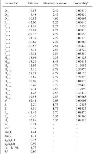
Estimation of genetic and nongenetic components of variation was carried out considering two nongenetic components and the ordinary least squares method. The error mean squares of the analyses of variance consider-ing only parents and only F1 hybrids were 8.79 and 19.20, respectively. The estimates are presented in Table III. Di-allel analysis indicated the presence of variability in the two parent groups, with type I error probability of approxi-mately 0.056 for group 2. Since D(1) - D(2) is positive (P = 0.09815), the genes that determine yield per plant are not equally frequent in the two parent groups. Genetic vari-ability is greater in group 1. Estimates of the mean values of the allelic gene frequency products, in the two groups, favor the previous inference. In group 1, there is evidence that allelic gene frequencies are close to 1/2 (uv = 0.24). In group 2, allelic genes have unequal frequencies (u’v’ = 0.17). Considering that mL0 - m’ = 3.32 (0.01 < P < 0.05), it can be concluded that yield-increasing genes have a fre-quency less than 1/2 in the second parental group. In short, the frequency of genes which increase trait expression is approximately 1/2 in group 1 and less in group 2, which explains the greater genetic variability found in the former. Parent F values from one group allow parents to be ranked according to the number of dominant genes they carry, not fixed in the other parental set. Ranking group 1
parents, according to an increasing concentration of domi-nant genes not fixed in group 2, the following order is obtained: Ricopardo 896, Ouro, DOR. 241, Ouro Negro, RAB 94 and Antioquia 8. Ricopardo 896, Ouro and DOR. 241 should have more recessive than dominant genes. Ouro Negro should have, approximately, similar numbers of dominant and recessive genes. RAB 94 and Antioquia 8 have more dominant than recessive genes. In group 2, the variety Batatinha carries the largest number of dominant genes, not fixed in group 1. Both BAT-304 and FT-84-835 should have dominant and recessive genes in approxi-mately equal numbers. Data indicate that recessive genes
Table III - Estimates of the genetic and non-genetic components of variation and of genetic parameters, in relation to grain yield of common
bean plants, in grams.
Parametera Estimate Standard deviation Probabilityb
D(1) 9.53 2.47 0.00310
D(2) 4.48 2.47 0.05630
D(3) 10.82 4.66 0.02665
Fr = 1 -45.06 7.27 0.00040
Fr = 2 -11.39 7.27 0.16150
Fr = 3 25.97 7.27 0.00910
Fr = 4 -28.75 7.27 0.00550
Fr = 5 21.37 7.27 0.02170
Fr = 6 -30.87 7.27 0.00380
Fs = 1 -10.56 7.54 0.20420
Fs = 2 -8.11 7.54 0.31720
Fs = 3 17.31 7.54 0.05550
H1(1) 18.94 9.35 0.04125
H1(2) 13.56 8.43 0.07615
H2r = 1 11.95 9.79 0.13085
H2r = 2 5.10 9.79 0.30970
H2r = 3 28.27 9.79 0.01170
H2r = 4 5.89 9.79 0.28370
H2r = 5 25.09 9.79 0.01870
H2r = 6 6.49 9.79 0.26420
H2s = 1 9.34 9.53 0.17990
H2s = 2 4.23 9.53 0.33410
H2s = 3 19.55 9.53 0.03965
h2 62.41 7.05 0.00005
E 2.20 1.75 0.12455
E’ 4.80 1.75 0.01425
F(1) -11.45 5.70 0.08470
F(2) -0.46 6.37 0.94560
H2 12.88 6.35 0.04110
uv 0.24 -
-u’v’ 0.17 -
-h/d(1) 1.41 -
-h/d(2) 1.74 -
-kD/kR(1) 0.15 -
-kD/kR(2) 0.97 -
-(k+ - k--)2/k 1.77 -
-R2 0.99 -
-auv: Average value of the allelic frequency products in group 1. u’v’:
Aver-age value of the allelic frequency products in group 2. h/d(1): AverAver-age degree of dominance in group 1. h/d(2): Average degree of dominance in group 2. kD/kR (1): Proportion between dominant and recessive genes in group 1. kD/kR (2): Proportion between dominant and recessive genes in group 2. (k+ - k-)2/k: Indicator of the direction of dominance. R2: Determi-nation coefficient. bBased on the t-test with seven degrees of freedom. Table II -Summary of the regression analyses of Wr on Vr and of Ws on
Vs, regression coefficient estimates and significance level of the test of the hypothesis H0: β1 = 1a, in relation to grain yield of common
bean plants, in grams.
Mean square Source of variation d.f. Group 1 Group 2
Intercept 1 25.26+ 6.51+
Regression 1 189.51** 25.34*
Errorb 4.42 0.06
Coefficient 0.74+ 0.86++
aUsing the t statistic, with four and one degrees of freedom (d.f.) for the
error in the analyses considering groups 1 and 2, respectively. bWith four
and one degrees of freedom in the analyses for groups 1 and 2, respec-tively. **P < 0.01; *0.01 < P < 0.05; +0.05 < P < 0.10; ++P > 0.10.
Table I -Grain yield per plant, in grams, of nine common bean lines and their hybrids.
Parent
Parent BAT-304 FT-84-835 Batatinha
(1) (2) (3)
6.10 4.48 9.54
Ricopardo 896 (1) 9.26 10.11 7.46 16.57 Ouro Negro (2) 8.23 9.48 11.67 15.89 Antioquia 8 (3) 14.77 17.96 18.45 15.29 DOR. 241 (4) 13.55 7.79 9.58 15.62
RAB 94 (5) 8.41 12.16 9.85 9.46
Ouro (6) 5.87 7.82 11.23 16.39
L0
generally act to decrease plant yield, while dominant ones increase yield. This fact, established in the analysis of vari-ance (not presented), seems to be corroborated by the esti-mate of h2D
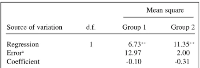
(1)D(2)/H2D2 , which indicates unidirectional dominance, despite its small magnitude. The regression analyses of pr on (Wr + Vr) and ps on (Ws + Vs), however, do not confirm the above information. The results of these regression analyses, using the observed parent means as the genotypic values, are in Table IV.
Estimates of the regression coefficients show the presence of statistically nonsignificant positive unidirec-tional dominance. This seems to indicate that many non-fixed dominant genes act to decrease yield, although the majority of them increase it. Estimates of the average de-gree of dominance are larger than one, although previous results indicate complete dominance. It is reasonable, there-fore, to admit that they are statistically equal to one. As there is evidence of complete dominance, estimates of the proportion among dominant and recessive genes suggest that the parents in group 1 have, on average, more reces-sive than dominant genes, while in group 2 the parents have, on average, the same number of recessive and domi-nant genes. These results agree with those from the analy-ses of the parent F values, as the majority of the parents in group 1 have more recessive than dominant genes, while in group 2 the majority have equal numbers of dominant and recessive genes.
The estimated F value for group 1 indicates that recessive genes, not fixed in group 2, are more frequent than dominant alleles. Taking the previous results into consideration, it can be concluded that this superiority is small. The estimate of F(2) suggests that dominant and re-cessive alleles, not fixed in group 1, are equally frequent in group 2, which is inconsistent with previous results. The presence of bi-directional dominance and fixed genes in the two parent groups may cause conflicting results in the genetic analysis. Many dominance component estimates show, as expected, the presence of dominance in the poly-genic system under study. H2 values of RAB 94, Antioquia 8 and Batatinha show that these genotypes are rare in their respective groups. They carry the least frequent genes in
their respective groups which are not fixed in the other group of parents. As already seen, they have more domi-nant genes than other parents in their group.
The difference between H2 values of RAB 94 and Antioquia 8 is nil (P = 0.30045), indicating that they have similar genotypes, in regard to yield determining genes. The cross between them should not result in relevant het-erosis, although it may be carried out to combine its nonfixed desirable genes in a single variety. As they have many dominant genes, which are rare in their group and not fixed in group 2, both can be used in crosses with the Batatinha variety, of group 2, which also has many domi-nant genes, rare in its group and not fixed in group 1. Es-timates of specific heteroses show that RAB 94 and Antioquia 8 genotypes are not completely distinct from that of the variety Batatinha (not presented). The small magnitude of the two specific heteroses, nil from a statis-tical point of view, is not surprising, since these varieties have more dominant than recessive genes. Values of the varietal heteroses indicate that RAB 94 has more frequent genes of group 2 than Antioquia 8, while Batatinha has less frequent genes in group 1 than FT-84-835 and BAT-304 (not presented).
Use of RAB 94 and Batatinha and/or Antioquia 8 and Batatinha as parents is justifiable if the objective of the program is to obtain pure lines. This objective would combine, in a single line, the favorable dominant genes which are not fixed in the parents. The smaller variability expected in the segregant generations derived from crosses between Antioquia 8 and RAB 94 and, preferably, between Antioquia 8 and RAB 94 with Batatinha could favor se-lection of a line with superior gene combination, contain-ing the favorable dominant and recessive nonfixed genes from both parents. Crosses of RAB 94, Antioquia 8 and Batatinha, with parents with many recessive genes, even in the same group, should show high levels of heterosis, due to their genotypic differences. If the objective is pro-duction of hybrids, several crosses, such as Antioquia 8 with FT-84-835 or BAT-304 and Batatinha with Ouro or Ricopardo 896 or Ouro Negro, may be considered. These crosses could also be considered in programs for pure lines, as there are various recessive genes that increase yield. Due to the accentuated genetic variability expected in the segregant generations of these crosses, it is necessary to use large number of plants and/or families to increase the probability of selecting a variety with a superior combina-tion of genes.
RESUMO
Neste trabalho são apresentadas teoria e análise de dialelos parciais, com base nos métodos propostos por Hayman em 1954 e 1958. A análise dialélica com os dados dos pais e de seus híbridos F1 possibilita uma caracterização detalhada dos sistemas poligênicos sob estudo e a escolha de progenitores para hibridação. A partir da estimativa de componentes genéticos e não genéticos da variação e de parâmetros genéticos, a análise (3)
Table IV - Summary, for each group of common bean lines, of the regression analyses of the parent genotypic value on the sum of the
variance and covariance in its array, in relation to grain yield per plant, in grams.
Mean square Source of variation d.f. Group 1 Group 2
Regression 1 6.73++ 11.35++
Errora 12.97 2.00
Coefficient -0.10 -0.31
aWith four and one degrees of freedom (d.f.) in the analyses of group 1 and
dialélica permite avaliar: a variabilidade genética em cada grupo; as diferenças genotípicas entre pais de grupos distintos; se um genitor tem genótipo comum ou raro no grupo ao qual não pertence; se há dominância; a direção de dominância; o grau médio de dominância em cada grupo; a importância relativa dos efeitos médios dos genes e dos desvios de dominância em determinar a característica; as freqüências de genes alélicos em cada grupo; se os genes são igualmente freqüentes nos dois grupos; o grupo em que os genes favoráveis estão em maior freqüência; o grupo em que os genes dominantes são mais freqüentes; o número relativo de genes dominantes e recessivos em cada pai; se um genitor tem genótipo comum ou raro em seu grupo, e as diferenças genotípicas entre os pais de um mesmo grupo.
REFERENCES
Chung, J.H. and Stevenson, E. (1973). Diallel analysis of the genetic varia-tion in some quantitative traits in dry beans. New Zealand J. Agric. Res. 16: 223-231.
Comstock, R.E. and Robinson, H.F. (1948). The components of genetic variance in populations. Biometrics 4: 254-266.
Comstock, R.E. and Robinson, H.F. (1952). Estimation of average domi-nance of genes. In: Heterosis (Gowen, J.W., ed.). Iowa State College Press, Ames, Iowa, pp. 494-516.
Coughtrey, A. and Mather, K. (1970). Interaction and gene association
and dispersion in diallel crosses where gene frequencies are unequal.
Heredity 25: 79-88.
Dickson, M.H. (1967). Diallel of seven economic characters in snap beans.
Crop Sci. 7: 121-124.
Gardner, C.O. and Eberhart, S.A. (1966). Analysis and interpretation of the variety cross diallel and related populations. Biometrics 22: 439-452.
Gilbert, N.E.G. (1958). Diallel cross in plant breeding. Heredity 12: 477-492.
Griffing, B. (1956). Concept of general and specific combining ability in relation to diallel crossing system. Austr. J. Biol. Sci. 9: 463-493.
Hayman, B.I. (1954). The theory and analysis of diallel crosses. Genetics 39: 789-809.
Hayman, B.I. (1958). The theory and analysis of diallel crosses. II. Genet-ics 43: 63-85.
Hayman, B.I. (1960). Maximum likelihood estimation of genetic compo-nents of variation. Biometrics 16: 349-381.
Jinks, J.L. (1954). The analysis of continuous variation in a diallel cross of
Nicotiana rustica varieties. Genetics 39: 767-788.
Jinks, J.L. and Hayman, B.I. (1953). The analysis of diallel crosses. Maize Genet. Coop. NewsL. 27: 48-54.
Kempthorne, O. and Curnow, R.N. (1961). The partial diallel cross. Bio-metrics 17: 229-250.
Kornegay, J.L. and Temple, S.R. (1986). Inheritance and combining abil-ity of leafhopper defense mechanism in common bean. Crop Sci. 26: 1153-1158.
Mather, K. and Jinks, J.L. (1974). Biometrical Genetics. 2nd edn. Cornell University Press, Ithaca, New York.
Nassar, R.F. (1965). Effect of correlated gene distribution due to sampling on the diallel analysis. Genetics 52: 9-20.
Nishimura, M. and Hamamura, K. (1993). Diallel analysis of cool
toler-ance at the booting stage in rice varieties from Hokkaido. Jpn. J. Breed. 43: 557-566.
Sokol, M.J. and Baker, R.J. (1977). Evaluation of the assumptions required for the genetic interpretation of diallel experiments in self-pollinat-ing crops. Can. J. Plant Sci. 57: 1185-1191.