Asian Online Journals (www.ajouronline.com) 236
Distribution of the Affinity Coefficient between Variables based on the
Monte Carlo Simulation Method
Áurea Sousa1, Osvaldo Silva 2, Helena Bacelar-Nicolau 3, Fernando C. Nicolau4 1
Department of Mathematics, CEEplA and CMATI, University of Azores, 9501-855-Ponta Delgada, Portugal
2
Department of Mathematics, CMATI, University of Azores, 9501-855-Ponta Delgada, Portugal,
3
Laboratory of Statistics and Data Analysis, FP, University of Lisbon, 1649-013-Lisboa, Portugal
4
Department of Mathematics,
FCT, New University of Lisbon, 2829-516-Caparica, Portugal
_________________________________________________________________________________
ABSTRACT— The affinity coefficient and its extensions have both been used in hierarchical and non-hierarchical
Cluster Analysis. The purpose of the present empirical study on the distribution of the basic and the generalized
affinity coefficients and on the distribution of the standardized affinity coefficient, by the method of Wald and
Wolfowitz, under different assumptions, is to assess the effect of the statistical probability distributions of the variables (columns) of the initial data matrix, and of the respective parameters, in the distribution of the values of these coefficients. We present some results concerning the asymptotic distribution of the referred coefficients under the assumption that the variables (for which the values of these coefficients are calculated) are independent and have statistical probability distributions specified apriori. In this distributional study, based on the Monte Carlo simulation method, we considered ten well-known statistical probability distributions with different variations of the respective parameters. The simulation studies lead to the conclusion that the coefficients’ convergence for the normal distribution is quite fast and, in general, a good approximation is obtained for small sample sizes, that is for sample sizes above 20 and in many cases for sample sizes above 10.
Keywords— Affinity coefficient, Pearson's correlation coefficient, Monte Carlo simulation method, probability laws
_________________________________________________________________________________
1. INTRODUCTION
To evaluate the proximity between two objects / variables in the scope of the Cluster Analysis, the choice of a measure based on distances or similarities is closely linked to the nature of the data. In the case of the clustering of variables, measures of similarity, such as the cosine of the angle between two vectors, the Pearson correlation coefficient and the affinity coefficient (Matusita [18, 19], Bacelar-Nicolau [3]), are usually applied.
One of the major drawbacks of the use of the correlation coefficient as a similarity measure is its sensitivity to shape at the expense of the magnitude of differences between the variables. Other limitation of the correlation coefficient is it often fails to satisfy the triangle inequality (Aldenderfer and Blashfield [2]). Moreover, the correlation coefficient only measures linear relationships between two variables. If the relationship is not linear, the use of Pearson correlation coefficient as a similarity measure between two variables, can conduct to inaccurate results.
The basic affinity coefficient takes values in the interval [0,1] and satisfy a set of proprieties which characterize affinity measurement as a robust similarity coefficient (e.g. Bacelar-Nicolau [6] and Bacelar-Nicolau et al. [7]. We continue a first empirical approach developed by F. C. Nicolau in 1994, on the asymptotic behaviour of the affinity coefficient. Even then it was crucial to invest in knowledge of the exact or asymptotic distributions of these coefficients, in order to approach the decision-process in Classification and the classical methods of statistical decision.
We developed a empirical study, based on the Monte Carlo simulation method, about the asymptotic distributions of the (basic/generalized) affinity coefficient, of the standardized affinity coefficient, by the method of Wald and Wolfowitz, and of the Pearson correlation coefficient, under the assumption that the vectors / variables / columns (for which the values these coefficients are calculated) are independent and follow probabilistic models (statistical probability distributions)defined a priori.
Asian Online Journals (www.ajouronline.com) 237
The Section 2 is devoted to the (basic/generalized) affinity coefficient, and to the standardized affinity coefficient, by the method of Wald and Wolfowitz. In Section 3, we describe the methodological framework of the present study. On the assumption of independency of the variables, the Pearson correlation coefficient assumes values close to zero, independently of the probability distribution of the variables and of the considered parameters. Thus, in Section 4, we present only the main conclusions that summarize the asymptotic results related to the (basic / generalized) affinity coefficient. Finally, Section 5 provides some concluding remarks about the work and its results.
2. BASIC AND GENERALIZED AFFINITY COEFFCIENTS
In the case of classical data we consider a table T=[xij: i=1, …, n; j=1,…p] containing sequences of real numbers. Let
(Xj, Xj’), jj’, be a pair of variables. The affinity coefficient generalized to sequences of real numbers between Xj and Xj’, or equivalently among the sequences (x1j,…,xnj) and (x1j´,…,xnj´) is given by (Nicolau [4], Nicolau and Bacelar-Nicolau [22]):
n i j´ ij´ j ij j´ ij´ j ijx
x
.
x
x
x
x
.sign
x
x
sign
j, j´
A
1,
(1)where sign is the abbreviation of "signal", and:
i ij i ij j i j ij i j ijx
x
x
w
x
x
x
x
´ j´ ´ ´x
and
ith
,
1
;
1
.
In particular, in the case of sequences of positive real numbers, the formula (1) becomes simpler and corresponds to the basic affinity coefficient (Matusita [18]; Bacelar-Nicolau, [3, 4]):
n i j´ ij´ j ijx
x
.
x
x
j, j´
A
1.
(2)The coefficients given by the formulas (1) and (2) take values, respectively, in the intervals [-1,1] and [0,1], and satisfy a set of proprieties which characterize the affinity measurement as a robust similarity coefficient.
Bacelar-Nicolau studied the asymptotic distribution of the affinity (Matusita [18, 19]) between variables, under different reference assumptions (e.g. Bacelar-Nicolau [3, 4]). In fact, Bacelar-Nicolau defined a probabilistic affinity coefficient in the scope of the VL methodology (V for Validity, L for Linkage) of Cluster Analysis (Lerman [16, 17], Bacelar-Nicolau [3, 4], Nicolau [20], Nicolau and Bacelar-Nicolau [21]), in particular under two hypotheses based, respectively, on the limit theorem of Wald and Wolfowitz (Fraser [12]) and on the limit theorem of delta-method (Tiago de Oliveira [23]).
The standardized affinity coefficient based on the limit theorem of Wald and Wolfowitz can be used as a similarity coefficient. The formula corresponding to this coefficient is the following (Bacelar-Nicolau [3, 4]):
2 1 ´ ´ ´ ´ 2 1 1 1 '1 ´ ´ ´1
1
1
1
'
,
n i j i j n i ij j n i n i n i j í ij ij ij Wx
n
x
x
n
x
x
x
n
x
x
n
j
j
A
.
(3)Later, Bacelar-Nicolau extended the affinity coefficient to complex data (symbolic data) and variables of mixed types (heterogeneous data), with different weights (Bacelar-Nicolau [5], Bacelar-Nicolau et al. [7,8]).
The comparison of clustering structures in the scope of Cluster Analysis has showed that methods based on the affinity coefficient are quite robust. Other advantage of this coefficient is its versatility and adaptability to different assumptions and different data types (Bacelar Nicolau et al. [7,8]).
3. METHODOLOGICAL FRAMEWORK
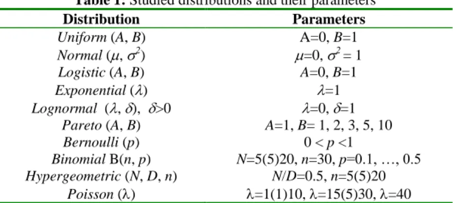
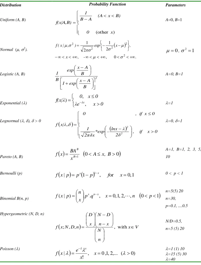
We used the Monte Carlo simulation method for the generation of pseudo-random numbers following ten well-known statistical probability distributions (Uniform, Normal, Logistic, Exponential, Lognormal, Pareto, Bernoulli, Binomial, Hypergeometric, and Poisson), with different variations of the respective parameters (see Table 1 and Table A.1 in
Asian Online Journals (www.ajouronline.com) 238
Appendix A). In this study, conducted using vectors of different dimensions, we considered in each case 50 samples of 500 values of the analysed coefficients, obtained from 500 pairs of independent vectors. For instance, we calculated the values of each one of the coefficients between columns 1 and 2, 3 and 4… and 999 and 1000, to ensure the independence of the sample of the values of these coefficients.
Table 1: Studied distributions and their parameters
Distribution Parameters
Uniform (A, B) A=0, B=1
Normal (, 2) =0, 2 = 1
Logistic (A, B) A=0, B=1
Exponential () =1
Lognormal (, ), >0 =0, =1
Pareto (A, B) A=1, B= 1, 2, 3, 5, 10
Bernoulli (p) 0 < p <1
Binomial B(n, p) N=5(5)20, n=30, p=0.1, …, 0.5 Hypergeometric (N, D, n) N/D=0.5, n=5(5)20
Poisson () =1(1)10, =15(5)30, =40
Measures of central tendency, quantiles, measures of dispersion, measures of skewness and kurtosis were calculated for the values of the different coefficients. The Kolmogorov–Smirnov test (K–S test) was also applied to each vector of values of these coefficients. The rectangular (uniform) continuous distribution is widely used as the basis for the generation of random numbers for other statistical distributions. In this study, the generation of random numbers uniformly distributed on [0, 1] was based on the combination of two multiplicative linear congruential generators (MLCG), that is of the type
x
j1
ax
jmod
m
, with m=2147483563, a=40014, and m=2147483399, a=40692,respectively. Therefore, the period of the combined generator is approximately 2.3 1018. The algorithm with the given values of m1, m2, a1 and a2 has been subjected to the spectral test and to many other tests by L’Ecuyer [15], who has provide a PASCAL version. He determined that it satisfied all of the requirements of the tests (Brandt [9]).
The generation of pseudo-random numbers following the standard normal distribution was based on the polar method by Box and Muller [10], and the generation of pseudo-random numbers with Binomial distribution with parameters n and
p was done using the method of Kemp [14].The used computer subroutines to generate pairs of vectors with
hypergeometric distribution (N, D, n) are the following functions:
i) r_hyperg (Dagpunar [11]), which is a simple method that is suitable when Min (n, D) is small (<=10).
ii) h_alias (Kachitvichyanukul et al. [13]), which is much faster for larger values of Min (n, D).
The subroutine used to generate pseudo-random numbers with Poisson distribution is a function subprogram, called "random_Poisson", adapted from RANLIB (Library of FORTRAN Routines for Random Number Generation). This function was compiled and written by Barry W. Brown and James Lovato and Translated to FORTRAN 90 by Alan Miller from RANLIB. For more details, see Ahrens [1].
4. RESULTS AND DISCUSSION
The counts can lead to the following distributions: binomial, hypergeometric and Poisson, in which the variance or covariance values are near zero and the limit is always the normal distribution. For this reason, special attention is given to the analysis of results obtained in the case of the generation of pseudo-random numbers obeying these laws. On the other hand, and with respect to continuous distributions, special emphasis is given to the Uniform distribution on [0,1] and the Normal distribution (0.1)
Generation of random numbers uniformly distributed on [0, 1]
In the case of the generation of vectors (columns) containing pseudo-random numbers uniformly distributed on [0, 1] we concluded that the arithmetic mean of the affinity coefficient is asymptotically convergent to the value 0.889 and that the standard deviation tends to the value 0.005. The distribution is approximately symmetric, and naturally the symmetry tends to be more pronounced for vectors of dimension greater than 30. The distribution is asymptotically normal and lognormal for vectors of dimension greater than 20, but the p-value is in general lower, as we could hope, in the case of the normal distribution. Obviously, the curve is frequently leptokurtic.
Generation of random numbers with standard normal distribution
By far the most important distribution for data analysis is the normal (Gaussian) distribution and it is possible to transform a random variable with normal distribution with mean and standard deviation in another random variable with standard normal distribution.
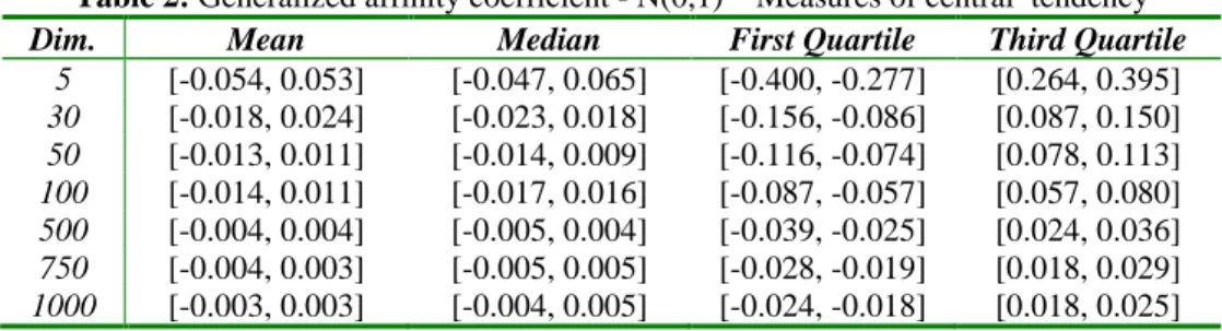
Asian Online Journals (www.ajouronline.com) 239 Table 2: Generalized affinity coefficient - N(0,1) – Measures of central tendency
Dim. Mean Median First Quartile Third Quartile
5 [-0.054, 0.053] [-0.047, 0.065] [-0.400, -0.277] [0.264, 0.395] 30 [-0.018, 0.024] [-0.023, 0.018] [-0.156, -0.086] [0.087, 0.150] 50 [-0.013, 0.011] [-0.014, 0.009] [-0.116, -0.074] [0.078, 0.113] 100 [-0.014, 0.011] [-0.017, 0.016] [-0.087, -0.057] [0.057, 0.080] 500 [-0.004, 0.004] [-0.005, 0.004] [-0.039, -0.025] [0.024, 0.036] 750 [-0.004, 0.003] [-0.005, 0.005] [-0.028, -0.019] [0.018, 0.029] 1000 [-0.003, 0.003] [-0.004, 0.005] [-0.024, -0.018] [0.018, 0.025]
In the case of the generation of vectors containing random numbers normally distributed as N(0,1), under the considered reference hypothesis, the mean and median of the generalized (to integer data) affinity coefficient tend to zero (see Table 2). Moreover, as the dimension (dim) of the vectors increases, the values of the affinity coefficient are increasingly concentrated around its average value (zero) (see Table 3).
Table 3: Generalized affinity coefficient - N(0,1) - Measures of dispersion
Dim. Interquartile
Range
Minimum Maximum Standard
Deviation 5 [0.604, 0.740] [-0.997, -0.925] [0.936, 0.999] [0.425, 0.467] 30 [0.209, 0.290] [-0.715, -0.430] [0.442, 0.663] [0.168, 0.203] 50 [0.163, 0.212] [-0.523, -0.342] [0.343, 0.565] [0.128, 0.148] 100 [0.123, 0.152] [-0.388, -0.240] [0.236, 0.431] [0.093, 0.107] 500 [0.054, 0.068] [-0.191, -0.108] [0.111, 0.161] [0.042, 0.048] 750 [0.042, 0.057] [-0.150, -0.085] [0.088, 0.162] [0.034, 0.038] 1000 [0.038, 0.047] [-0.016, -0.079] [0.080, 0.122] [0.030, 0.034]
Figure 1: Distribution of the Affinity Coefficient in the case of vectors of size 1000 containing pseudo-random numbers following the standard normal distribution
The histogram obtained in the first repetition involving 500 values of the affinity coefficient, obtained from vectors of dimension 1000 following the standard normal distribution, N(0,1), are plotted in Figure 1.
Table 4- Quantiles of the generalized affinity coefficient- N(0,1)
Dim. Q0.005 Q0.01 Q0.025 Q0.05 Q0.1 Q0.25 Q0.5 Q0.75 Q0.90 Q0.95 Q0.975 Q0.990 Q0.995 5 -0.944 -0.923 -0.844 -0.743 -0.598 -0.334 -0.002 0.332 0.596 0.738 0.853 0.914 0.946 30 -0.473 -0.431 -0.359 -0.305 -0.240 -0.128 -0.001 0.122 0.236 0.300 0.356 0.413 0.461 50 -0.359 -0.329 -0.273 -0.231 -0.181 -0.097 -0.002 0.094 0.180 0.230 0.274 0.316 0.365 100 -0.255 -0.236 -0.193 -0.164 -0.128 -0.068 0.002 0.068 0.129 0.163 0.195 0.228 0.254 500 -0.115 -0.106 -0.088 -0.074 -0.058 -0.031 0.000 0.030 0.057 0.073 0.087 0.102 0.116 750 -0.094 -0.087 -0.072 -0.060 -0.046 -0.025 0.000 0.025 0.047 0.059 0.071 0.084 0.095 1000 -0.082 -0.074 -0.062 -0.053 -0.040 -0.021 0.000 0.021 0.041 0.052 0.062 0.073 0.080 The distribution is symmetric (see Table 4), and the curve is frequently leptokurtic. The use of K-S test allowed us to confirm that the distribution of the generalized (to integer data) affinity coefficient is asymptotically normal and that for sample sizes greater than 20 the approximation is generally quite good.
Asian Online Journals (www.ajouronline.com) 240 Generation of random numbers with binomial distribution
We obtained vectors of pseudo-random numbers, with Binomial distribution with parameters n and p, of dimension
10, 30, 50, 100, 250, 500 and 1000, considering the parameters n=5, 10, 15, 20 and 30 and p= 0.1 (0.1) 0.9. However, we
present only the asymptotic values obtained for the mean, standard deviation and interval of variation of the basic affinity coefficient for the case of vectors of dimension 1000 (see Table B.1 in Appendix B).
In this empirical study, we concluded that once the value of parameter n was fixed, the higher the value of p is, the higher are the values obtained for the basic affinity coefficient. On the other hand, the standard deviation of the basic affinity coefficient is very low, regardless of the distribution parameters and of the vectors’ dimension, and it tends to get lower in the following cases: increase of the vectors’ dimension, increase of the value of n and increase of the value of p.
When the vectors obey to the law B (15, 0.9) (respectively, B (30, 0.9)) there is a clear convergence of the values of affinity coefficient to value 0.998 (respectively, 0.999). On the other hand, in the cases of vectors with distributions
B(5, 0.9) and B(10, p) with 0.8 p 0.9, B(15, p) with 0.7 p 0.9, B(20, p) with 0.6 p 0.9, and B(30, p) with 0.5 p 0.9, the asymptotic standard deviation is approximately zero.
Generation of random numbers with Poisson distribution
The study considered the generation of pairs of vectors with Poisson distribution for various values of , (=1 (1) 9,
=10 (5) 30 and =40), based on the Monte Carlo simulation method, and it was considered for each of these values of
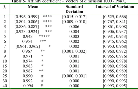
the generation of vectors of dimension 10, 30, 50, 100, 250, 500, 750 and 1000. The asymptotic values obtained for the mean value, standard deviation and interval of variation of the basic affinity coefficient are shown in Table 5. As the value of gets higher, it can be observed that:
- The mean value of the affinity coefficient also increases;
- The speed of convergence to the asymptotic mean value increases, although it should be noted that, for example, for
=25, 30 and 40, this convergence is already verified from vectors of dimension 30;
- The standard deviation of the affinity coefficient decreases, and for =30 (from vectors of dimension 750) and for
=40 (from vectors of dimension 500), the value of the standard deviation is approximately zero (0000). Table 5- Affinity coefficient – Vectors of dimension 1000 - Poi()
Mean Standard Deviation Interval of Variation 1 [0.596, 0.599] **** [0.015, 0.017] [0.529, 0.666] 2 [0.804, 0.806] **** [0.009, 0.010] [0.767, 0.841] 3 [0.886, 0.887] *** 0.006 [0.861, 0.908] 4 [0.923, 0.924] *** 0.004 [0.906, 0.937] 5 0.943 ***** 0.003 [0.931, 0.953] 6 0.954 *** 0.002 [0.945, 0.962] 7 [0.961, 0.962] * 0.002 [0.953, 0.968] 8 0.967 ** [0.001, 0.002] [0.960, 0.972] 9 0.971 * 0.001 [0.965, 0.976] 10 0.974 * 0.001 [0.969, 0.978] 15 0.983 * 0.001 [0.980, 0.986] 20 0.987 ** 0.001 [0.985, 0.989] 25 0.990 # [0.000, 0.001] [0.988, 0.992] 30 0.992 # 0.000 [0.990, 0.993] 40 0.994 # 0.000 [0.993, 0.995]
# - value (s) obtained from vectors of dimension 30 and on.
* - value (s) obtained from vectors of dimension 100 and on. ** - value (s) obtained from vectors of dimension 250 and on. *** - value (s) obtained from vectors of dimension 500 and on. **** - value (s) obtained from vectors of dimension 750 and on. ***** - value (s) obtained from vectors of dimension 1000 and on. Generation of random numbers with hypergeometric distribution
In the case of the generation of vectors with hypergeometric distribution, the empirical study was conducted for vectors of dimension 1000 and D/N = 0.5, taking into account several possible values for the parameters N, D and n.
Asian Online Journals (www.ajouronline.com) 241
Keeping D / N constant, for example equal to 0.5, it appears that in the case of vectors of dimension 1000, the higher the value of the parameter n is, the higher tends to be the mean value of the basic affinity coefficient (see Table B.2 in Appendix B). Then, with D = 1000 and N = 500, we considered vectors of dimension 10, 30, 50, 100, 250, 500, 750 and 1000 and values of the parameter n (sample size) equals to 5, 10, 15 and 20. It was found that from vectors of dimension 30 and on, the values of the measures of central tendency and the values of the measures of dispersion are already very close to those obtained for vectors of dimension 1000, especially for n15. The standard deviation of the
basic affinity coefficient is very small.
The present study showed that when N is large compared with n, the binomial distribution provides a good approximation for the hypergeometric distribution, as was expected based on the Theory of Probabilities. The distribution of the basic affinity coefficient is approximately symmetric, even though it presents a slight tendency to be negatively skewed. The curve is frequently leptokurtic, whatever the dimension of the vectors. This coefficient tends to follow asymptotically the normal distribution and the lognormal distribution.
Summary of results for other studied distributions
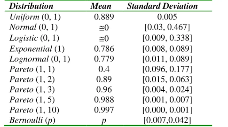
The main conclusions about the means and standard deviations of other distributions studied are summarized in Table 6. Note, in particular, that in the case of the Pareto distribution with location parameter equal to 1, the increase of the shape parameter causes an increase in the mean value of the affinity coefficient and a decrease in the value of the standard deviation of this coefficient (that is, a great concentration of values around the mean).
The empirical study, on the asymptotic distribution of the affinity coefficient in the case of binary data, allowed us to confirm, as we might expect in accordance with theory, that the mean of the values of the affinity coefficient between pairs of independent vectors following the Bernoulli distribution with parameter p tends asymptotically to p. In the case of the basic/generalized affinity coefficient, the curve is frequently leptokurtic and in most cases the distribution tends to follow the normal distribution and the lognormal distribution (in general, with a value of p-value lower for the normal distribution). Additional details about the obtained results (including other tables) can be found in Sousa [24].
Table 6- Mean value and standard deviation of the generalized affinity coefficient – other distributions
Distribution Mean Standard Deviation
Uniform (0, 1) 0.889 0.005 Normal (0, 1) 0 [0.03, 0.467] Logistic (0, 1) 0 [0.009, 0.338] Exponential (1) 0.786 [0.008, 0.089] Lognormal (0, 1) 0.779 [0.011, 0.089] Pareto (1, 1) 0.4 [0.096, 0.177] Pareto (1, 2) 0.89 [0.015, 0.063] Pareto (1, 3) 0.96 [0.004, 0.024] Pareto (1, 5) 0.988 [0.001, 0.007] Pareto (1, 10) 0.997 [0.000, 0.001] Bernoulli (p) p [0.007,0.042] 5. CONCLUSION
The mean value and the standard deviation of the standardized affinity coefficient based on the limit theorem of Wald and Wolfowitz do not depend on the kind of distribution of the vectors nor of the parameters of the distribution. This coefficient tends to follow asymptotically the normal distribution and the Student’s distribution, except on what concerns the Pareto distribution (1, 1). The distribution is approximately symmetric, even though in the case of this coefficient it presents a slight tendency to be positively skewed.
The mean values and the standard deviations of the (basic and generalized) affinity coefficient depend on the statistical probability distributions of the variables. As we could hope, their variability is associated with the sample size, being greater when the sample size is reduced. The values of the basic affinity coefficient tend to follow asymptotically the normal distribution and the lognormal distribution, except for the Pareto distribution with parameters (1, 1) and (1, 2), being the p-value, as we might expect, in general lower in the case of the normal distribution. On the other hand, the generalized affinity coefficient tends to follow asymptotically the normal law. The curves are approximately symmetrical, but have a slight tendency to be negatively skewed.
The simulation studies lead to the conclusion that the coefficients’ convergence for the normal distribution is quite fast and, in general, a good approximation is obtained for sample sizes above 20 and in many cases for sample sizes
Asian Online Journals (www.ajouronline.com) 242
above 10. This last propriety of the affinity coefficient is very important when we deal with probabilistic models based on asymptotic distributions such as the one based on the limit theorem of Wald and Wolfowitz. Furthermore, in the scope of cluster validation, the knowledge of the asymptotic distribution of the basic and the generalized affinity coefficients can potentiate the development of a hypothesis test in order to test the null hypothesis of absence of structure of the data.
6. REFERENCES
[1] Ahrens, J. H. and Dieter, U., “Computer Generation of Poisson Deviates From Modified Normal Distributions”, ACM Trans. Math. Software, vol. 8, no.2, pp.163-179, 1982.
[2] Aldenderfer, M. and Blashfield, R., Cluster Analysis, Sage University Paper, 44, 1984.
[3] Bacelar-Nicolau, H., “Contribuições ao Estudo dos Coeficientes de Comparação em Análise Classificatória”, PhD Thesis, FCL, Universidade de Lisboa, 1980.
[4] Bacelar-Nicolau, H., “Two Probabilistic Models for Classification of Variables in Frequency Tables”, In: Bock, H. H. (Eds.), Classification and Related Methods of Data Analysis. North Holland, pp. 181-186, 1988.
[5] Bacelar-Nicolau, H., “The Affinity Coefficient”, In: Analysis of Symbolic Data: Exploratory Methods for Extracting Statistical Information from Complex Data, H.-H. Bock and E. Diday (Eds.), Berlin: Springer-Verlag, pp. 160-165, 2000.
[6] Bacelar-Nicolau, H., “On the Generalised Affinity Coefficient for Complex Data.Biocybernetics and Biomedical Engineering”, vol. 22, no. 1, pp. 31-42, 2002.
[7] Bacelar-Nicolau, H.; Nicolau, F.C.; Sousa, Á.; Bacelar-Nicolau, L., “Measuring Similarity of Complex and Heterogeneous Data in Clustering of Large Data Sets”, Biocybernetics and Biomedical Engineering, vol. 29, no. 2, pp. 9-18, 2009.
[8] Bacelar-Nicolau, H.; Nicolau, F.C.; Sousa, Á.; Bacelar-Nicolau, L., “Clustering Complex Heterogeneous Data Using a Probabilistic Approach”, In Proceedings of Stochastic Modeling Techniques and Data Analysis International Conference (SMTDA2010), published on the CD Proceedings of SMTDA2010 (electronic publication), 2010. [9] Brandt, S., Data Analysis – Statistical and Computational Methods for Scientists and Engineers, Third ed., Springer -
Verlag, New York, 1999.
[10] Box, G. E. P. and Muller, M. E., “A Note on the Generation of Random Normal Deviates”, Annals of Mathematical Statistics, vol. 29, no. 2, pp. 610-611, 1958.
[11] Dagpunar, J., Principles of Random Variate Generation, Clarendon Press, Oxford, United Kingdom, 1988. [12] Fraser, D. A. S., Non Parametric Methods in Statistics, Chapman and Hall, pp. 235-237, 1975.
[13] Kachitvichyanukul, V., Schmeiser, B., “Computer Generation of Hypergeometric Random Variates”, Journal of Statistical Computation and Simulation, vol. 22, pp. 127-145, 1985.
[14] Kemp, C. D., “A Modal Method for Generating Binomial Variables”, Commun. Statist. - Theor. Meth, vol. 15, no. 3, pp. 805-813, 1986.
[15] L’Ecuyer, P., “Efficient and Portable Combined Random Number Generators”, Communications of the ACM, vol. 31, no. 6, pp. 742-751, 1988.
[16] Lerman, I. C., “Sur l`Analyse des Données Préalable à une Classification Automatique”, Rev. Math. et Sc. Hum., vol . 32, no. 8, pp. 5-15, 1970.
[17] Lerman, I. C., Classification et Analyse Ordinale des Données, Paris, Dunod, 1981.
[18] Matusita, K., “On the Theory of Statistical Decision Functions”, Ann. Instit. Stat. Math., vol. III, pp. 1-30, 1951. [19] Matusita, K., “On the Notion of Affinity of Several Distributions and Some of its Applications”, Annals of
Mathematical Statistics, vol. 19, no. 2, pp. 181-192, 1967.
[20] Nicolau, F. C., “Cluster Analysis and Distribution Function”, Methods of Operations Research, vol. 45, pp. 431-433, 1983.
[21] Nicolau, F. C. and Bacelar-Nicolau, H., “Some Trends in the Classification of Variables”, In: Hayashi, C., Ohsumi, N., Yajima, K., Tanaka, Y., Bock, H.-H., Baba, Y. (Eds.), Data Science, Classification, and Related Methods. Springer-Verlag, pp. 89-98, 1998.
[22] Nicolau, F. C., Bacelar-Nicolau, H., “Teaching and Learning Hierarchical Clustering Probabilistic Models for Categorical Data”, Online IASE and ISI Conference Proceedings, IASE at ISI, 54, IPM-71, 2003.
[23] Tiago de Oliveira, J., “The -Method for Obtention of Asymptotic Distributions”, Applications. Public. Inst. Statist, Univ. Paris, vol XXVII, pp. 49-70, 1982.
[24] Sousa, Á., “Contribuições à Metodologia VL e Índices de Validação para Dados de Natureza Complexa”, PhD Thesis, Universidade dos Açores, 2005.
Asian Online Journals (www.ajouronline.com) 243 APPENDIX A
Tabela A.1. Studied distributions and their parameters
Distribution Probability Function Parameters
Uniform (A, B) ) (other x 0 B) x (A A B 1 f(x|A,B) A=0, B=1 Normal (, 2).
. , x , x exp ) , | x ( f 2 2 2 2 2 0 , 2 1 2 1 0
,
2
1
Logistic (A, B) 2 B A x exp 1 B A x exp B 1 A=0, B=1 Exponential ()
0
x
λe
0
x
0
f(x|λ
x,
,
)
=1 Lognormal (, ), > 0
0 x , if 2δ λ lnx -*exp δx 2π 1 0 , if x 0 x|λ f 2 2 , =0, =1 Pareto (A, B)
B1 Bx
BA
x
f
0
A
x
,
B
0
A=1, B=1, 2, 3, 5, 10 Bernoulli (p)
|
1
1,
or
0
,
1
x
f
p
p
p
x
f
x x 0 < p < 1 Binomial B(n, p)(
|
)
.
.
,
0
,
1
,
2
,
,
0
1
p
n
x
q
p
x
n
p
x
f
x n x
n=5(5) 20 n=30, p=0.1, ....0.5 Hypergeometric (N, D, n)
x V n N x n D N x D n D N x f , with , , ; N/D=0.5, n=5 (5) 20 Poisson ()
,
0
,
1
,
2
,...
(
0
)
!
|
x
x
e
x
f
x =1 (1) 10 =15 (5) 30 =40Asian Online Journals (www.ajouronline.com) 244
APPENDIX B
Table B.1. Affinity coefficient - vectors of dimension 1000 - B(n, p)
n=5 p Mean Standard Deviation Interval of Variation 0.1 [0.396, 0.400] [0.020, 0.024] [0.310, 0.486] 0.2 [0.641, 0.644] [0.014, 0.016] [0.584, 0.696] 0.3 [0.788, 0.790 [0.010, 0.011] [0.741, 0.829] 0.4 [0.875, 0.877] [0.006, 0.008] [0.841, 0.903] 0.5 [0.926, 0.927] [0.004, 0.005] [0.905, 0.944] 0.6 0.956 0.003 [0.943, 0.966] 0.7 0.974 [0.001, 0.002] [0.967, 0.980] 0.8 [0.985, 0.986] 0.001 [0.982, 0.989] 0.9 0.994 0.000 [0.992, 0.995] n=10 p 0.1 [0.618, 0.621] [0.014, 0.017] [0.557, 0.682] 0.2 [0.838, 0.840] [0.008, 0.009] [0.804, 0.874] 0.3 [0.921, 0.922] [0.004, 0.005] [0.902, 0.938] 0.4 0.955 [0.002, 0.003] [0.943, 0.964] 0.5 0.972 [0.001, 0.002] [0.965, 0.977] 0.6 0.982 0.001 [0.978, 0.985] 0.7 [0.988, 0.989] 0.001 [0.986, 0.991] 0.8 0.993 0.000 [0.992, 0.995] 0.9 0.997 0.000 [0.996, 0.998] n=15 p 0.1 [0.745, 0.747] [0.011, 0.013] [0.699, 0.791] 0.2 [0.909, 0.910] [0.005, 0.006] [0.889, 0.928] 0.3 0.955 [0.002, 0.003] [0.944, 0.965] 0.4 0.973 0.001 [0.967, 0.978] 0.5 0.982 0.001 [0.979, 0.986] 0.6 0.988 0.001 [0.986, 0.990] 0.7 [0.992, 0.993] 0.000 [0.991, 0.994] 0.8 0.996 0.000 [0.995, 0.996] 0.9 0.998 0.000 [0.998, 0.998] n=20 p 0.1 [0.821, 0.823] [0.008, 0.009] [0.782, 0.855] 0.2 [0.939, 0.940] [0.003, 0.004] [0.925, 0.952] 0.3 0.968 [0.001, 0.002] [0.962, 0.974] 0.4 0.980 0.001 [0.976, 0.983] 0.5 0.987 0.001 [0.984, 0.989] 0.6 0.991 0.000 [0.990, 0.993] 0.7 0.994 0.000 [0.993, 0.995] 0.8 0.997 0.000 [0.996, 0.997] 0.9 0.999 0.000 [0.998, 0.999] n=30 p 0.1 0.898 [0.005, 0.006] [0.876, 0.920] 0.2 [0.963, 0.964] 0.002 [0.955, 0.970] 0.3 [0.979, 0.980] 0.001 [0.975, 0.984] 0.4 0.987 0.001 [0.984, 0.989] 0.5 0.991 0.000 [0.990, 0.993] 0.6 0.994 0.000 [0.993, 0.995] 0.7 0.996 0.000 [0.996, 0.997] 0.8 0.998 0.000 [0.997, 0.998] 0.9 0.999 0.000 [0.999, 0.999]
Asian Online Journals (www.ajouronline.com) 245 Table B.2. Basic affinity coefficient - H(N, D, n )
Dim. Mean Standard
Deviation Interval of Variation N=1000; D=500; n=5 10 [0.926, 0.934] [0.042, 0.051] [0.659, 0.998] 30 [0.926, 0.931] [0.024, 0.028] [0.774, 0.990] 50 [0.926, 0.930] [0.019, 0.022] [0.818, 0.979] 100 [0.926, 0.928] [0.013, 0.015] [0.860, 0.968] 250 [0.926, 0.928] [0.009, 0.010] [0.886, 0.958] 500 [0.926, 0.928] [0.006, 0.007] [0.896, 0.952] 750 [0.926,0.928] [0.005, 0.006] [0.903,0.947] 1000 [0.926, 0.927] [0.004, 0.005] [0.907, 0.943] N=1000; D=500; n=10 10 [0.973, 0.976] [0.013, 0.017] [0.841, 0.999] 30 [0.972, 0.974] [0.008, 0.009] [0.912, 0.994] 50 [0.972, 0.973] [0.006, 0.007] [0.934, 0.992] 100 [0.972, 0.973] [0.004, 0.005] [0.947, 0.985] 250 [0.972, 0.973] [0.003, 0.003] [0.957, 0.983] 500 [0.972, 0.973] [0.002, 0.002] [0.961, 0.980] 750 [0.972, 0.972] [0.002, 0.002] [0.965, 0.979] 1000 [0.972, 0.972] [0.001, 0.002] [0.966, 0.977] N=1000; D=500; n=15 10 [0.983, 0.985] [0.008, 0.009] [0.911, 0.999] 30 [0.983, 0.983] [0.004, 0.005] [0.956, 0.995] 50 [0.982, 0.983] [0.004, 0.004] [0.961, 0.994] 100 [0.982, 0.983] [0.003, 0.003] [0.969, 0.990] 250 [0.982, 0.983] [0.002, 0.002] [0.975, 0.988] 500 [0.982, 0.983] [0.001, 0.001] [0.978, 0.987] 750 [0.982, 0.983] [0.001, 0.001] [0.978, 0.986] 1000 [0.982, 0.983] [0.001, 0.001] [0.979, 0.986] N=1000; D=500; n=20 10 [0.988, 0.989] [0.005, 0.006] [0.949, 0.999] 30 [0.987, 0.988] [0.003, 0.004] [0.965, 0.997] 50 [0.987, 0.988] [0.002, 0.003] [0.971, 0.995] 100 [0.987, 0.987] [0.002, 0.002] [0.979, 0.993] 250 [0.987, 0.987] [0.001, 0.001] [0.982, 0.991] 500 [0.987, 0.987] [0.001, 0.001] [0.983, 0.991] 750 [0.987, 0.987] [0.001, 0.001] [0.984, 0.990] 1000 [0.987, 0.987] [0.001, 0.001] [0.984, 0.989]