WORKING PAPER SERIES
CEEAplA WP No. 05/2008
Labor Market Regulations and Trade Patterns:
the Panel Data Analysis within a Modified
Ricardian Setting
Ainura Uzagalieva
Labor Market Regulations and Trade Patterns:
the Panel Data Analysis within a Modified
Ricardian Setting
Ainura Uzagalieva
Universidade dos Açores (DEG)
CEEAplA e CERGEI-EI
Working Paper n.º 05/2008
Maio de 2008
CEEAplA Working Paper n.º 05/2008 Maio de 2008
RESUMO/ABSTRACT
Labor Market Regulations and Trade Patterns: the Panel Data Analysis within a Modified Ricardian Setting
The paper focuses on the question of how labor market regulations can affect a country’s competitive position in international trade and international trade patterns. The analysis shows that differences in labor market flexibility between countries affect their competitive positions in international markets and can serve as an independent cause of international trade. It is argued that an increase in labor market flexibility may change the relative price of goods within the country making it more competitive in international markets for commodities with uncertain demand. Changes in relative prices can alter countries’ comparative advantage and thus international trade patterns. Furthermore, it is shown that due to the differences in relative prices resulting from different labor market regulations, international trade between countries can be observed even if they are identical in all respects (e.g., labor productivity and production technology). Data reveal that a country with a more flexible labor market has comparative advantage in, and tends to export, goods with more variable demand (e.g., fashionable clothes, seasonal toys), while a country with a more rigid labor market has a comparative advantage in, and tends to export, commodities with more stable demand.
JEL Classification: F100, D800
Ainura Uzagalieva
Departamento de Economia e Gestão Universidade dos Açores
Rua da Mãe de Deus, 58 9501-801 Ponta Delgada
Labor Market Regulations and Trade Patterns: the Panel Data Analysis
within a Modified Ricardian Setting *
Ainura Uzagalieva**
(CEEAplA, CERGE-EI)
Abstract
The paper focuses on the question of how labor market regulations can affect a country’s competitive position in international trade and international trade patterns. The analysis shows that differences in labor market flexibility between countries affect their competitive positions in international markets and can serve as an independent cause of international trade. It is argued that an increase in labor market flexibility may change the relative price of goods within the country making it more competitive in international markets for commodities with uncertain demand. Changes in relative prices can alter countries’ comparative advantage and thus international trade patterns. Furthermore, it is shown that due to the differences in relative prices resulting from different labor market regulations, international trade between countries can be observed even if they are identical in all respects (e.g., labor productivity and production technology). Data reveal that a country with a more flexible labor market has comparative advantage in, and tends to export, goods with more variable demand (e.g., fashionable clothes, seasonal toys), while a country with a more rigid labor market has a comparative advantage in, and tends to export, commodities with more stable demand.
JEL Classification: F100, D800
*The preliminary version of this paper was published in Economia Enternazionale/International Economics, 2006, Vol. LIX, No. 2.
** I am indebted to Jacek Cukrowski for his collaboration and valuable comments in developing this paper. I am also grateful to Randal Filer, Lubomir Lizal, Sergej Slobodyan, Kresmir Zigic, and Sarah Peck for useful comments and suggestions. All mistakes and misprints are mine.
1. Introduction
International trade plays a key role in the strategies of poverty reduction, economic growth and affects overall national development. In many cases, however, geographical location, high transportation costs or the lack of advanced technologies do not allow countries to benefit from international exchange. There exist regions where countries with similar technological levels, climate conditions and regulatory framework, lacking a clear comparative advantage, compete with each other on international markets and, except for some trade in natural resources, cannot fully explore benefits of international exchange within and outside the region.
Most of the factors (e.g., geographical location, high transportation costs, climate conditions, and the lack of advanced technologies) that affect countries’ comparative advantage cannot be changed by policymakers. However, appropriate institutional settings and regulations determining business conditions can increase economic efficiency, decrease domestic prices of selected products, and thus, increase a country’s price competitiveness on international markets. Although general links between business environment and price competitiveness seem to be clear, the impact of various policy measures on producers and market prices needs to be clarified in many cases. This study focuses on the relation between labor market regulations, international competitiveness,1
and patterns of trade. Specifically, we argue that policy measures which increase labor market flexibility may change the relative price of goods within a country, making it more competitive in international markets for commodities with volatile demand,2 and, consequently, that flexibility of the labor market can be considered an important factor that would stimulate exports of a broad range of products, especially those with high demand volatility.
Another important theoretical point to be gained from this study is that since an increase in labor market flexibility may change the relative price of goods within the
1We refer to the academic definition of international competitiveness which is: “Competitiveness of
Nations is a field of Economic theory, which analyzes the facts and policies that shape the ability of a nation to create and maintain an environment that sustains more value creation for its enterprises and more prosperity for its people” [see International Institute for Management Development (IMD) World Competitiveness Yearbook (WCY): 2003].
2The group of products with volatile demand includes seasonal products (e.g., processed meat, fish, fruit,
country, it can also alter countries’ comparative advantage and thus international trade patterns. In particular, we show that due to the differences in relative prices, which result from different labor market regulations, international trade between countries can be observed even if the countries are identical in all respects (e.g., labor productivity, production technology, and consumption preferences). The analysis reveals that a country with a more flexible labor market has comparative advantage in, and tends to export, goods with more variable demand, while a country with a more rigid labor market has comparative advantage in, and tends to export, commodities with more stable demand.
The analysis presented in this paper has been motivated by an observation that within a single industry commodities with relatively stable demand are produced throughout the world, while very similar goods with more volatile demand are produced in particular countries only. One can think about the textile or toy industry where products with relatively stable demand (e.g., traditional clothing) are produced in both developed (with high wages) as well as developing (with low wages) countries, while technologically similar products with more volatile demand (e.g., ethnic-style clothing, toys, cards, CDs, and similar products such as movie tie-ins, for example, Star Wars, Matrix, The Lord of the Rings, and Harry Potter) are produced exclusively in developing countries with very liberal labor market regulations.3 Another example includes the
export of watches and clocks,4 which have more stable demand on the world markets and are produced throughout the world, versus agricultural goods with high variability such as meat, fish, fruit, vegetables, and fats which have a larger share in the exports of developing countries. This simple example shows that large scale production of goods with volatile demand, and their export to international markets, may significantly
3The market for such products is huge. To illustrate the scale, one can consider solely the market for Harry
Potter related products, where the total earnings (until the summer of 2003) from the sales of books, movies, video tapes, CDs, video games, and clothes exceeded 3.5 billion USD. In other words, the total earnings from such products exceed the yearly GDP of a number of developing countries (for comparison, the GDP of the Kyrgyz Republic amounted to 1.7 billion USD in 2003). See the International Bank for Reconstruction and Development/the World Bank (IBRD/WB), 2005: World Development Indicators (WDI).
4The comparison of export shares (61 products) across 37 countries based on the standard deviation of each
product’s sales shows that the watches and clocks group has the lowest variation (0.001), while the group of processed meat, fish, fruit, vegetables, and fats has the highest variation of sales (0.194) during the period from 1995 to 2002.
improve countries’ balance of payments and could have a positive impact on the economy as a whole.
The paper is organized as follows. Section 2 highlights the concept of labor market flexibility. Section 3 focuses on the speed of labor market adjustment to new market conditions. An autarky regime in a simple Ricardian setting under price uncertainty is analyzed in section 4. Section 5 explores the impact of labor market flexibility on international trade. In section 6 key theoretical results are confronted with empirical data and section 7 concludes.
2. The concept of labor market flexibility
The concept of labor market flexibility refers to various phenomena and can be defined by at least three of the following important dimensions (Hamermesh 1996; Pissarides 1997). First, it is related to organizational and productive aspects at the company level, namely, to the ability of a firm to vary its production volume and to introduce new models and products. Second, it refers to the capacity and skills of employees (e.g., building multiple skills, training workers for different production operations, and tasks). Third, it is applied to employment policies, wage adjustments, changes in work schedules, and hiring and firing procedures consistent with production needs.5 Labor market flexibility is also related to the population aging phenomenon since old workers are generally less mobile and incur high costs resulting from firms’ adjustment to demand shocks (Kuhn 2003).
Although labor market flexibility can be related to several phenomena, it can be characterized by the speed of adjustment in response to various shocks in an economy (Pissarides 1997). The virtue of the latter is that one labor market is more flexible than the other one if it adjusts to a given shock faster. In a perfectly flexible labor market, workers are free to allocate their services in response to shifting relative wage opportunities, while firms are free to adjust the workforce in response to shifting relative profit opportunities. Moreover, it is assumed that both workers and firms adapt immediately to any changes in market conditions and in labor demand.6
5These include, for example, contracts for certain tasks, part-time work or at-home work.
6Departing from a neoclassical model (perfectly flexible labor market), decreasing labor market flexibility
In real life, however, there are several constraints that limit the ability of firms and workers to quickly adjust to changing market conditions and labor demand. Employment protection is one of them. It refers to hiring and firing practices on unfair dismissals, lay-off restrictions, severance payments, minimum notice periods, and security against job dismissals. Employment protection can originate from various institutional arrangements. When labor markets are not regulated, employment protection is based on wage compensation schemes and collective bargaining. Namely, firms with high dismissal rates pay workers a compensating wage for occupational hazards. This fact causes firms to implement either an adjustment strategy, through retraining workers and marginal regulations (e.g., attrition, early retirement, work sharing, and severance payments), or firing workers and accepting higher compensating wages. The problems of permanent lay-offs are dealt by unions which represent a collective bargaining mechanism for protecting work places. However, when markets fail (e.g., externalities, imperfect competition, insufficient information, and public goods), the wage compensation mechanism and collective bargaining do not work. In this case governments legislate employment protection through imposing restrictions of different kinds. According to the World Bank (WB), the constraints of labor market flexibility can be ordered from the most (1) to the least (5) severe: 1) hiring difficulties; 2) hours rigidities; 3) firing difficulties; 4) employment rigidities; and 5) firing costs.7
Three basic types of employment protection measures are distinguished in the literature (Bertola, Boeri, Cazes 1999; Boeri, Nicoletti, Scarpetta 2000; Hamermesh 1996). The first type includes provisions affecting fixed costs per worker (e.g., the statutory guarantees of payments to workers, various agreements to limit overtime or provide shorter working time). The second type includes provisions that affect the cost of labor adjustment (e.g., redundancy payments, subsidies to retain employees and provisions for unfair dismissals).8 The third type consists of provisions affecting the process of labor adjustment such as lay-offs by inverse seniority, restrictions on hiring, and various pre-notifications regarding factory closings or redundancies.
7See the International Bank for Reconstruction and Development/the World Bank (IBRD/WB), 2005:
Doing business in 2005.
8Statutory rights against unfair dismissals exist in all countries except the United States (see Bertola, Boeri,
No matter what the type of employment protection and which institutional measures it originates from, any kind of employment protection arrangements, enforcing hiring and firing rules, unemployment benefits, and minimum wages are regarded as factors decreasing labor market flexibility. These factors constrain the free choice of workers and firms and increase the inertia of the labor market (i.e., reduce the speed of labor adjustment to new market conditions). Not going into the details of labor market regulations, in this paper, following Pissarides (1997), we assume that one labor market is more flexible than the other one if firms can faster adjust employment to the new market conditions.
3. The speed of labor market adjustment and a firm’s input-output decisions
As discussed in the preceding section, we assume that if the labor market is perfectly flexible, firms are able to adjust the amount of labor needed in the production process to observed market conditions immediately. Any decrease in labor market flexibility makes the adjustments of labor input slower, i.e., increases labor market inertia. Since labor market regulations are usually the same for all sectors in the economy, in the deterministic case (i.e., when the demand for goods is certain) they should have the same impact on all industries. Therefore, labor market regulations would not affect relative prices, and thus, a country’s comparative advantage. Under uncertainty of demand, however, all inputs in the production process which are not perfectly flexible (i.e., cannot be adjusted immediately) need to be chosen before the output is produced and the price of real output is observed. Provided that firms are not risk neutral, but risk-averse,9 the uncertainty about output price affects the optimal input/output decisions of
firms (Leland 1972; Yu and Ingene 1993) and, consequently, the relative prices of goods with different output price variability.
To clarify the relationship between the uncertainty of output price and firms’ optimal input/output decisions, consider a single commodity market and assume that the price of the unit of output produced is uncertain and can be represented as the sum of two terms, a fixed term (expected value) and a random term (ηt) at any period of time t (t is an
9A similar assumption was made by Sandmo (1971), Leland (1972), Cukrowski and Aksen (2003) and
Cukrowski, Fischer and Aksen (2002). As indicated by Leland, risk neutrality is frequently assumed just for the sake of simplicity (see Leland, 1972, for detailed discussion).
integer number such that −∞<t<+∞). For the sake of simplicity, assume that the random
variables (ηt) are identically distributed with zero mean and finite variance (σt2). Assume,
moreover, that the random deviations from the mean price (ηt) are described by a
stationary stochastic process with a memory (e.g., by the auto-regressive processes of any order). This means that the variance and covariance of random variables (ηt) are invariant
with respect to displacement in time (i.e., Var(ηt)=Var(η)=σ2>0, Cov(ηt,ηt+s)≠0 for
s=0,1,..., and integer valued t (−∞<t<+∞), and that firms can observe real values of ηt at
each period).
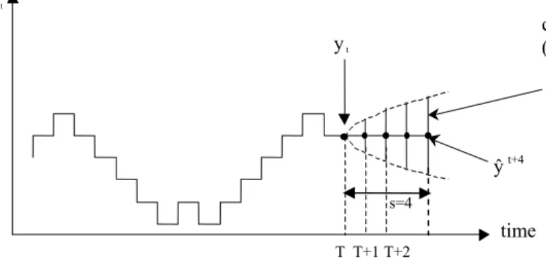
Since various labor market regulations, which result in a different degree of labor market flexibility, affect the speed of labor adjustment to changing market conditions, they also determine the time interval needed for labor input fine-tuning. In other words, the degree of labor market flexibility determines the time length between the moment when a firm’s decision on its input/output plan is enacted and the moment when its output is supplied to the market and real output price is observed. Note that if the labor market is not perfectly flexible, the firm’s input/output decision needs to be made before the real demand is known (based on forecasts). Consequently, in the moment of decision making perceived market price variability is inversely related to the flexibility of the labor market. This is because the forecast error of deviation from an expected demand equals zero and its variance increases with the time elapsed from observations to the moment when real output price is revealed (Pindyck and Rubinfeld 1991). For example, if random deviations follow the first-order autoregressive process [e.g., ηt=φ1ηt-1+εt,
where φ1 is a constant parameter and εt is a random disturbance term with zero mean
and variance σε2 under the normal distribution N(0, σε2)], the s period forecast
estimated in period T, ηtf(s), is ηtf(s)=φ1sηT. The forecast error of s periods ahead, eT(s),
is given as eT(s)=εT+s+φ1εT+s-1+…+φ1s-1εT+1, and it has a variance
E[eT(s)2]=(1+φ12+φ14+...+φ12s-2)σε2, which increases (nonlinearly) as s becomes larger
Figure 1. Forecast errors in a first-order autoregressive process
4. Price uncertainty and an autarky regime in a Ricardian setting
For the sake of simplicity the analysis which follows is based on the international trade model in a simple Ricardian setting. The original model is extended by assuming that demand for one good (out of two goods considered) is uncertain. More precisely, two goods, X and Y, are produced in a perfectly competitive environment, but there is always uncertainty about the price of the first good (X). The technology is summarized by the productivity of labor, which is expressed in terms of the unit labor requirement (i.e., the number of hours required to produce one unit of each good) in each industry. For future reference let us define aLX and aLY as the unit labor requirements in the production of X
and Y goods, respectively. The limits of production in this economy can be determined by the inequality
(1) aLXQX+aLYQY≤L,
where
(2) QX=LX/aLX , and
(3) QY=LY/aLY ,
denote, respectively, the quantities of goods X and Y produced in the economy; LX and LY
describe the amount of labor employed in the sectors X and Y, correspondingly; L is the total labor supply.
To determine what the economy will actually produce, one needs to know the expected relative price of goods. The price of good X is random and can be represented
T T+1 T+2 ŷt+4 y t y t time s=4 confidence interval (represented by 1 standard deviation)
as pX(θ), where θ is a stochastic parameter that characterizes the state of the world, such
that
(4) ,
where is the expected price of the commodity X. Thus, the supply of good X in the competitive economy is determined by the attempts of firms to maximize their expected utilities from profits. All firms are assumed to be managed by risk-averse managers10 and, therefore, their attitudes towards risk can be characterized in a von Neumann-Morgenstern fashion in the form of a utility function (Sandmo 1971; Leland 1972). Risk aversion implies that utility function U of profit π is strictly concave: U’(π)>0 and U’’(π)<0. Thus, each firm operating in industry X selects the quantity of output qx to
maximize the expected utility from profit
(5) { [ ( x)]}
q E U q
Max
x
π .
The first order condition (FOC) in a perfectly competitive environment can be represented as
(6)
where
(7) πX =[pX(θ)−waLX]qx,
and qX denotes output of a single firm and w stands for wage in the economy.
The second order condition (SOC) is
(8) = [ ''( )( ( )− )2]<0 LX X X p wa U E D π θ .
Rearranging FOC we get
(9) )] ( ' [ )] ( ) ( ' [ X X X LX U E p U E wa π θ π = .
Expression (9) allows us to prove the following important proposition:
Proposition 1. Under uncertainty, perfectly competitive firms equate marginal cost to a certain value bigger than the price under certainty (p ), i.e., X
(10) X X X X p U E p U E > )] ( ' [ )] ( ) ( ' [ π θ π .
10 See Mayer (1978) and Batra (1974).
X X p p E[ (θ)]= X p 0 , ]} ) ( )[ ( { ' − = LX X X p wa U E π θ
Proof:
Let '( )
X
U π be the marginal utility of profit for θ = , such that θ pX(θ)− pX =0. Since the marginal utility is decreasing and all profits are non-negatively correlated, we
must have that '( ) '( )
X X U
U π ≤ π for θ, such thatpX(θ)− pX ≥0. Multiplying both sides of the inequality above by pX(θ)− pX, we get
(11) '( )( ( ) ) '( )( ( ) ) X X X X X X p p U p p U π θ − ≤ π θ − . If pX(θ)− pX ≤0, then ( ) ( ) ' ' X X U
U π ≥ π , and consequently the sign in the last
inequality is unaffected. Taking expectation we have
(12) [ '( )( ( )− )]≤ '( ) [( ( )− )]=0 X X X X X X p p U E p p U E π θ π θ ,
and taking into account that
(13) [ '( )( ( )− )]= [ '( )( ( )]− [ '( )] ≤0 X X X X X X X p p EU p EU p U E π θ π θ π , we get (14) E[U'(πX)pX(θ)] E[U'(πX)]≥ pX. Q.E.D
An important implication of Proposition 1 is that the total output of industry X under uncertainty is smaller than it would be under certainty.
Perfect competition in industry Y (without uncertainty) implies that the price of the good Y, p , equals marginal cost: Y
(15) w= pY/aLY.
Since wage rates need to be equal across sectors, we have
(16) E[pX] pY =E[pX pY]≥ pX pY =aLX aLY .
It follows from the expression (16) that in industry X the expected relative price of goods
X and Y under uncertainty will be higher than in the certainty case.
The proposition below reveals a link between the magnitude of price fluctuations and the expected relative price of the goods X and Y. 11
11 The analysis presented in this paper can be replicated in a more general and more complex setting with
two sectors and two production factors (as in the Heckscher-Ohlin model of international trade), but the complexity of the model makes it hardly readable. As an example, a link between labor market flexibility, expected relative prices within the country, and country price competitiveness in international markets in the model with two sectors and two production factors is analysed in the appendix.
Proposition 2. An increase in the price variability of good X with uncertain demand decreases the amount of labor allocated to the production of commodity X and increases the expected relative price of goods X and Y.
Proof.
Consider the effect of a marginal increase in uncertainty on the demand for labor input. To present the notion of increased uncertainty, define an increased variability in the density function of the price of good X in terms of a “mean preserving spread,”12 i.e., define random variable pX* as
(17)
p
X*=
γ
p
X+
ϖ
,where pX* is a random price, ϖ and γ are shift parameters which initially equal zero and
unity, respectively. The mean preserving spread type of the shift in the density function of pX* leaves mean E[pX*] unchanged, that is
(18) dE[p* ]=dE[
γ
p +ϖ
]= p dγ
+dϖ
=0X X
X .
Substituting pX* by pX in the FOC of sector X, we obtain
(19) E[U′(πX)(γpX+ϖ-waLX)]=0,
where
(20) πX =[(γpX +ϖ)−waLX]qx.
Differentiating (20) with respect to γ and taking into account that
d
ϖ
d
γ
=
−
p
X we get(21) 1 [ ''( )( )( )] 1 [ '( )( )] X X X LX X X X X X X EU p p D wa p p p U E D q d dq =− π − − − π − γ ,
where D is the SOC determined by expression (8).
The second term in expression (21) is negative and the first term is generally indeterminate.13 However, in the particular case when we assume that the initial situation is such that
p
X=
p
X and an increased uncertainty causes only a very small increase in risk, then a certain price can be replaced by the probability distribution with all outcomes
12 Defining a change in uncertainty in terms of a change in the probability distribution, while keeping its
mean constant, is quite common in economic theory (see, for example, in Sandmo (1971), Rothenberg and Smith (1971), and Rothschild and Stiglitz (1970, 1971).
13At this level of formalization, making a clear statement on the marginal effect of uncertainty on output is
unlikely. To deal with this difficulty, one can focus on a particular case when the marginal impact of uncertainty is identical to its overall impact, i.e., when increased uncertatinty leads to just a little more risky distribuition than the initial one (see Sandmo 1971).
concentrated in the neighborhood of
p
X . And, if price is known to be equal top
X , the marginal cost is also equal top
X . So, we must have
p
X=
wa
LX , and (22) 1 [ ''( )( )( )] 1 [ '( )( )]. X X X X X X X X X X EU p p D p p p p U E D q d dq =− π − − − π − γ (23) − 1 [ ''( )( − )2]<0 X X X X EU p p D q π .Therefore, if the distribution of prices is concentrated around its mean value dqX /dγ <0, an increase in price volatility decreases the quantity of output produced and increases the expected price of good X.14 Taking into account that the price of good Y is deterministic, we conclude that an increase in the price variability of good X has two effects. First, since the quantity of output produced is proportional to the quantity of labor used, it decreases the amount of labor allocated to the production of commodity X. Second, it increases the expected relative price of goods X and Y.
Q.E.D.
One implication of Proposition 2 is that higher labor market flexibility resulting in a smaller time lag between the moment at which decision-making concerning labor is made and the moment at which the price of an output becomes known decreases the price of the good with uncertain demand, and thus makes the country more competitive in the international market for this commodity. This important result can be formulated as the following corollary:
Corollary 1. An increase in labor market flexibility makes a country more competitive in international markets for commodities with uncertain demand.
Proof.
As it is mentioned in section 3, lower market flexibility implies a slower adjustment of labor input to market conditions, and thus increases the time period between the moment when the firm’s input/output decision needs to be made and the
14 This result is consistent with Sandmo (1971) among others. We need to mention that Batra and Ullah
(1974) show that in any case an increase in uncertainty leads to a decline in the firm’s output if absolute risk aversion is decreasing.
moment when the output is supplied to the market and real output price is observed (see Figure 1). This in turn implies that if labor market flexibility decreases, the uncertainty about demand at the moment of decision making (and price variability) increases (and vice versa). Consequently, by Proposition 2, an increase in labor market flexibility decreases the expected relative prices of goods with uncertain demand with respect to ones with certain demand. In other words, higher labor market flexibility leads to the reduction of absolute prices of goods with uncertain demand, and, therefore, makes a country more competitive in international markets for the commodities with uncertain demand.
Q.E.D.
The other important implication of Proposition 2 is that differences in labor market flexibility, determining a time lag between the time when a decision concerning labor is made and the time when prices for output became known, and thus price variability in the time of decision making, lead to different expected relative prices, and, consequently, may change patterns of trade or cause international exchange of goods.
5. The impact of labor market flexibility on international trade patterns
Consider a world of two countries, A and B, and assume that each of the two countries has only one scarce factor of production (labor), and can produce two goods, X and Y. Production technologies are described by unit labor requirements aLiJ , where
J∈{A, B} and i∈{X,Y}. Assume that the unit price of commodity Y is deterministic and
the unit price of commodity X is uncertain. Suppose also that the labor market in country
A is more flexible than in country B, which implies that input/output decisions in sector X
in country B have to be made earlier than in country A, and, consequently, that deviation of expected relative prices from relative prices in the deterministic case in country B is always greater than in country A. This may change the pattern of trade predicted by the classical Ricardian model in the way described by one of the propositions below.
Proposition 3. Two countries, identical with respect to production technology and labor productivity, can be involved in international trade: the country with a
more flexible labor market will tend to export goods with uncertain demand, while the country with a more rigid labor market will tend to export goods with deterministic demand.
Proof.
Lack of differences in production technology and labor productivity imply that
(24) aLXA/aLYA=aLXB/aLYB,
i.e., in the deterministic case no country has a comparative advantage, and therefore international exchange of goods is not observed. Proposition 2 implies that under uncertainty higher labor market flexibility in country A will result in smaller expected relative prices in country A than expected relative prices in country B, and, consequently, country A will tend to export good X (with uncertain demand) while country B will tend to export good Y (with deterministic demand).
Q.E.D.
The Proposition 4 implies that a rational for international trade exists even if there is no comparative advantage in the sense of differences among countries in technology and labor efficiency. Under uncertainty, a difference in labor market flexibility is the only reason for comparative advantage and international exchange of goods.
Proposition 4. Under uncertainty, differences in labor market regulations may change trade patterns resulting from a comparative advantage in labor productivity and production technology.
Proof.
In the deterministic case, country B has a comparative advantage in producing X if
(25) aLXA/aLYA>aLXB/aLYB .
Consequently, country B has also lower relative prices of goods X and Y, and thus it exports good X in exchange for good Y. Proposition 2 implies that under uncertainty, expected relative prices in country A (with a more flexible labor market) may rise less than expected relative prices in country B (with a more rigid labor market), and, consequently, country A will tend to export good X while country B will tend to export good Y. So, in this case difference in labor market flexibility changes the trade pattern
predicted based on comparative advantage in labor productivity and production technology.
Q.E.D.
An important implication of Proposition 4 is that in the real world, where input/output decisions concerning production of most goods are made under uncertainty, trade patterns can differ from ones that follow from classical economic theory under certainty.
6. Empirical evidence
This section deals with empirical evidence where the following testable proposition is postulated: the share of export of the sectors with high variation of firm
sales increases with labor market flexibility. The hypothesis reflects theoretical results
formulated as Proposition 2, Corollary 1, and Proposition 3. In particular, a high degree of labor market flexibility allows firms facing demand uncertainty to more quickly adjust their production capacities to shifts in demand. The reallocation of labor across firms within a certain industry is reflected in the change of sales of firms and industry groups as well (see Proposition 2 and Corollary 1). Since in a country with a more flexible labor market the scale of firms’ adjustment is much higher (i.e., there are substantial labor and production shifts across industry groups), a country with a more flexible labor market tends to export more goods with variable demand (as indicated in Proposition 3). On the contrary, in a country with a more rigid labor market, labor and production shifts across industry groups are much smaller, and therefore, countries with a more rigid labor market tend to export goods with stable demand.
In order to test the hypothesis formulated above, we analyse the impact of labor market regulations on export demand variability within the manufacturing sector. The equation specification is of the following panel regression form:
(26) WVARit =α1+α2LMFit +uit,
where LMFit reflects the labor market flexibility index, uit is the error term, and the
dependent variable denotes the weighted variances of firms’ sales (WVARit), the fraction
weighted variation of a single firm’s sales, which are calculated across years, from the mean variation across all industries, whose export shares are taken as corresponding weights:
(27)
( )
(
)
( )
( )
, 1 , 1 1 , 1 : s.t. , 1 1 1 1 1 2 1 jt J j j T t T t jt jt jt j J j j J j j it j J j j it q VAR J VAR q T q T q VAR EX ex w VAR q VAR w WVAR∑
∑
∑
∑
∑
∑
= = = = = = = ⎟ ⎠ ⎞ ⎜ ⎝ ⎛ − = = = ⎥ ⎦ ⎤ ⎢ ⎣ ⎡ − =where I is a number of countries, T number of years, and J number of industries;
w is the weight or the share of an individual industry’s export (ex) in the total
exports of all industries (EX); q denotes the average sale of a single firm.
The hypothesis test is H0: α2=0, against H1: α2>0. That is, the fraction of an industry’s
exports with high variation of firms’ sales increases with the degree of labor market flexibility (i.e., α2 is positive).
By pooling all the available observations that cover data from 37 countries (I=37) including the values of exports, the number of establishments, the volume of sales across
61 manufacturing products (J=61), and the labor market flexibility indexes for the period
1995 to 2002 (T=8),15 the regression coefficients are estimated by ordinary least squares (OLS), random effect (RE) and fixed effect (FE) models. The data for the export products and the number of establishments come from the United Nations Industrial Development Organization’s (UNIDO) Industrial Statistics Database and national statistics offices databases at the three digit level of International Standard Industrial Classification (ISIC) of revision 2. As the proxy of labor market flexibility, the employment law indexes, which are presented in Global Competitiveness Yearbook (GCY) by the International Institute for Management Development (IMD) are used. Table 2 demonstrates the statistical moments of the main variables included in model estimation.
15A comparable data set is not yet available for 2003 and 2004 for all products and countries included in the
Table 1. Descriptive statistics of the variables used in the model
Minimum Maximum Median Mean Std. dev. Skewness Kurtosis LMF 1.1922 8.3612 4.7119 4.8109 1.3337 0.1781 2.6536 VWAR 0.0133 249.9037 6.6709 16.2196 25.5625 4.9215 39.5923 Source: the author’s calculations
In terms of statistical descriptors, which are presented in Table 2, the labor market flexibility indexes are characterized by better properties than those of the weighted variances. The labor market flexibility indexes, for example, range from a minimum of
1.1922 to a maximum of 8.3612 with a mean value of 4.8109 and a standard deviation of 1.3337, indicating that the presence of extreme outliers is not likely in the data. The
dependent variable, however, lies in a range from a minimum 0.0133 to a maximum
249.9037 with a mean of 16.2196 and a standard deviation 25.5625. Hence, in terms of
the third and fourth moments, labor market flexibility indexes are better distributed than the weighted variances, as demonstrated in Figure 2.
a) 0.00 0.05 0.10 0.15 0.20 0.25 0.30 2 4 6 8
LMF: Kernel Density (Normal, h = 0.3934)
b)
Figure 2. The shapes of distribution: a) LMF; b) WVAR
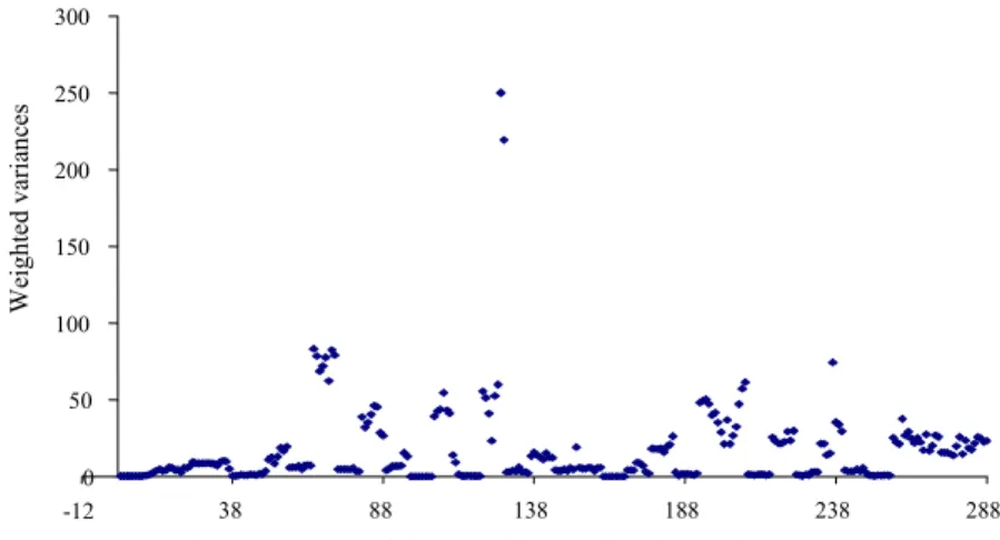
It follows from Figure 2 that the shape of the distribution plotted on the labor market flexibility indexes is closer to that of normal distribution, while the distribution of the weighted variations of firms’ sales is very leptokurtic with most of the data concentrated within a more narrow range.16 High kurtosis reflects few large values of the weighted variation of firms’ sales (see Figure 3).
Figure 3. Weighted variances in panel data
16Normal distributions are characterized by the kurtosis equal to 3 (see Green 2001).
0 50 100 150 200 250 300 -12 38 88 138 188 238 288
Number of observation in panel data: neighboring plots depict observations across years within a single country
We ight ed var ia nc es 0.00 0.01 0.02 0.03 0.04 0.05 0.06 0 50 100 150 200 250 WVAR: Kernel Density (Normal, h=4.0247)
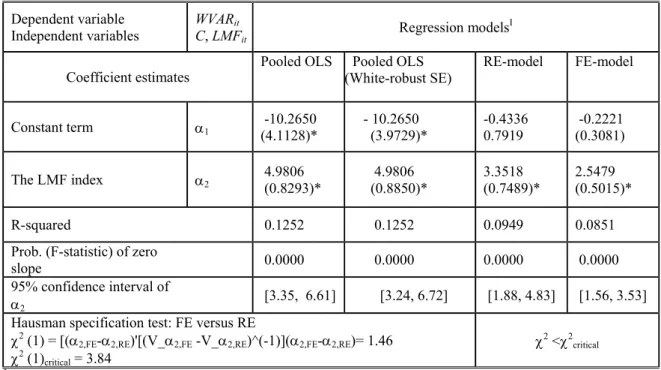
The comparison of weighted variances across countries identifies Hungary, where the variance increased from 60 to 260 in 2001, as an outlier in the sample data and, thus, it is excluded from the data set. The results of an econometric estimation are demonstrated in Table 3.
Table 2. The estimation parameters of OLS (the panel for I=36 countries and T=8 years)
Dependent variable
Independent variables WVARC, LMFit it Regression models
I
Coefficient estimates Pooled OLS (White-robust SE) Pooled OLS
RE-model FE-model
Constant term α1 -10.2650 (4.1128)* - 10.2650 (3.9729)* -0.4336 0.7919 -0.2221 (0.3081)
The LMF index α2 4.9806 (0.8293)* 4.9806 (0.8850)* 3.3518 (0.7489)* 2.5479 (0.5015)*
R-squared 0.1252 0.1252 0.0949 0.0851 Prob. (F-statistic) of zero
slope 0.0000 0.0000 0.0000 0.0000 95% confidence interval of
α2 [3.35, 6.61] [3.24, 6.72] [1.88, 4.83] [1.56, 3.53]
Hausman specification test: FE versus RE χ2 (1) = [(α
2,FE-α2,RE)'[(V_α2,FE -V_α2,RE)^(-1)](α2,FE-α2,RE)= 1.46
χ2 (1)
critical = 3.84
χ2 <χ2 critical IThe estimated asymptotic standard errors (SE) are shown in the brackets below the estimated coefficients:
(*) indicates a 1% significance level.
As Table 2 demonstrates, the results of pooled OLS reveal the presence of a positive first-order serial correlation in residuals as presented in Table 3 (the Durbin-Watson statistics is 0.07).17 The null hypothesis of homoscedasticity, which is tested by computing White statistics by regressing the squared least squares residuals on a constant, LMF, and LMF2
(NRT2=8.32∼χ2) is rejected in favor of the alternative hypothesis of heteroscedasticity.18 These findings suggest that standard errors and estimated coefficients are not valid to make an inference. Since the residuals are not independent, the RE model is applied, but first, the model with robust estimation is performed and regression models with robust standard errors are applied. The robust 95% confidence interval is wider than both the
17 The null hypothesis of no AR(1) serial correlation in OLS residuals is rejected at the 5% level. 18 The 5% critical value from the table for the chi-squared statistics with 2 degrees of freedom is 5.99.
previously estimated OLS and RE regression results by 0.22 and 0.53, correspondingly. In order to test the appropriateness of the RE estimator, we estimate the FE-model and perform a Hausman specification test.19 As reported in Table 3, the reported χ2 value is smaller than the critical value, so that the H0 cannot be rejected at the 5% significance level. This suggests that the RE-model is the preferred option for making an inference.
Based on the results obtained by the RE-model, one can infer that an 1 point higher degree of labor market flexibility corresponds to a 3.35 point larger variation of firm sales weighted by export industry export shares. The estimated R2 explains about
9.94% of the variation. The empirical evidence confirms the presence of a significant
positive relationship between labor market flexibility and the export shares of sectors with high variation of firms’ sales. This can imply that firms respond to demand fluctuations by reallocating inputs to the production of goods with higher world demand which causes an increase in the variation of sales across firms as well as industry groups. As a result, a country with more flexible labor market is more competitive in goods with flexible demand and exports more goods with higher variation of sales due to the fact that the scale of firms’ adjustment is much higher and there are substantial labor and production shifts across industry groups. On the contrary, in a country with a more rigid labor market, the variation of exports across industry groups is smaller due to lower adjustment speed. Therefore, countries with a more rigid labor market tend to export goods with more stable demand.
7. Conclusion
The analysis above explored the links between labor market regulations and prices of commodities with uncertain demand, relative prices within the country and patterns of trade. It has been shown that since flexible labor market regulations allow companies to adapt to changes in demand quickly, firms’ decisions regarding labor input may be made based on better predictions (i.e., under smaller uncertainty), which improves economic efficiency leading to better allocation of resources. This in turn leads to lower prices of the commodities with uncertain demand within countries and makes
19The hypothesis test is that the individual country-specific effects are uncorrelated with the other
them more competitive on international markets for these products. Since in the real world, suppliers of most commodities and services face uncertain demand, a high degree of labor market flexibility may significantly increase competitiveness of all countries including those with high wage levels. On the contrary, rigid labor market regulations may increase prices for most goods and services within countries and thus decrease competitiveness of these countries, even those with relatively low wages.
These theoretical results have been confronted with empirical evidence and a positive correlation between labor market flexibility and export variation across product groups has been confirmed. This implies that in response to world demand shifts, countries with flexible labor markets can reallocate labor across industry groups towards production of goods with higher demand. This causes an increase in the variation of sales across firms and industry groups as well. As a result, countries with more flexible labor markets export more goods with higher variation of sales due to the fact that the scale of firms’ adjustment is much higher. On the contrary, in countries with more rigid labor markets, the variation of exports across industry groups is smaller due to lower adjustment speed, and the exports of goods with more stable demand is larger. The link between labor market flexibility and relative prices of goods in autarky explored in the paper reveals also that there would be a justification for international trade between identical countries even if markets are perfectly competitive. International exchange of goods with different price variability may stem from differences in labor market institutional settings. Simple analysis of possible trade patterns in a modified Ricardian setting shows that even if countries are similar in all respects (e.g., labor productivity or technology), but have differences in labor market regulations, then international trade among these countries can be observed, and a country with a flexible labor market will tend to export goods with variable demand, while a country with a rigid labor market will tend to export goods with stable demand.
Since an increase in labor market flexibility has a positive impact on countries’ international competitiveness and thus on their balance of trade, a number of actions which may help liberalize labor markets can be recommended to both developed and developing counties. Generally, measures for increasing labor market flexibility require policy actions on several different levels. Firstly, removing the sources of labor market
rigidities through institutional arrangements and changes in labor legislation at the macro level is widely recommended. The policy actions at this level involve measures for reducing the power of unions, the role of collective bargaining, and the level of employment protection. From the perspective of labor market flexibility at the intra-enterprise level, regulations can be accomplished through increasing wage and working hours flexibility, eliminating incentives for wage arrears, restructuring social assets, and using such active adjustment mechanisms as training and retraining policies. Such measures ease the movement of workers from one job to another and lower the cost of dismissals by inducing employers to fire workers with obsolete skills and hire new workers. It needs to be emphasized, however, that policy actions in a concrete country or region should be designed taking into account the specific environment, including macroeconomic conditions, the level of market development, value system, cultural heritage and many other factors.
There are many ways in which this study can be extended and generalized. In particular, the problem considered in the paper can be presented in a broader framework using a standard two countries, two commodities and two production-factors model (Heckscher-Ohlin model). Such an analysis, although quite complicated (see Appendix), can lead to a number of interesting conclusions regarding, e.g., the impact of labor market regulations on relative prices of labor and capital intensive commodities with different demand uncertainty, predictions of the Heckscher-Ohlin theorem and the Rybczynski theorem, as well as on the distribution of welfare within trading countries, and thus on poverty reduction.
Appendix Labor market flexibility and relative prices of goods in a two factors and two sectors model under uncertainty
Consider a single economy with two perfectly competitive sectors, one of them producing a commodity X and the second one – a commodity Y. There are two factors of production: capital (K) and labor (L) available in fixed supply. Assume that production technology in the sectors X and Y can be characterized by Cobb-Douglass production functions fX and fY: fX(KX,LX)= LXα KX1-α (0<α<1) and fY(KY,LY)= LYβ KY1-β (0<β<1),
where LX, KX and LY, KY are the amounts of labor and capital employed in the industries X
and Y, respectively. Following the analysis presented in Section 4, all firms are assumed to be managed by risk-averse managers and, therefore, their attitudes towards risk can be characterized in a von Neumann-Morgenstern fashion in the form of a utility function [risk aversion implies that utility function U of profit π is strictly concave: U’(π)>0 and U’’(π)<0]. Consumption patterns can be derived from the following utility functions U(QX, QY) = QXσ QY1-σ (0<σ<1), where QX, QY denote the quantities of goods X and Y
consumed, respectively; but in the analysis which follows we assume that the demand of commodity X is always uncertain, while the demand of commodity Y is known for sure at any moment of time.
In order to simplify the analysis, following the considerations presented in Section 3, assume that an error term in the prediction of price is a normally distributed random variable with zero mean and variance σt2 (this corresponds to the case when random
deviations follow stochastic processes with normally distributed random terms such as, for example, the autoregressive process of any order).20 Since the distribution of the total
random deviation from the mean value of price is normal, the total deviation can take a positive or a negative value, each having probability ½. Namely, the expected values of a
20 It should be stressed that although the assumption of the normal distribution of the random deviations
from the expected price corresponds to the wide class of stochastic processes that would govern stochastic price movement, it is chosen solely for simplicity and clarity, and no attempt is made at generality. We believe, however, that many of the qualitative results would hold also in more general, and, consequently, more complicated models.
positive and a negative value equal σt/ 2π and −σt/ 2π , correspondingly.21
Consequently, the price of commodity X at any time t (such that -∞<t<+∞) can be
approximated as Px+ϑ(σt), whereϑ(σt) is a random factor (not known ex-ante) that equals θ(σt) with probability ½ and -θ(σt) with probability ½, respectively [θ(σt)
=σt/ 2π ]. So, the price of commodity X is presented as Px−θ(σt) with probability ½ and P+θ(σt) with probability ½. In such a framework we can prove the following proposition:
Proposition A1. An increase in labor market flexibility decreases the expected relative price of goods X with respect to good Y and makes the country more competitive in international markets for a commodity with uncertain demand.
Proof.
Perfect competition implies that the profits of all firms operating in industry Y (with certain demand) equal zero. The cost function of firms operating in industry Y is described as
C(Y)=aKYr+aLYw. (A.1)
The terms r and w in the expression (A.1) denote the price of capital and labor, and aK,Y
and aL,Y are the amounts of capital and labor needed to produce one unit of commodity Y,
respectively.
To allocate resources, the firms operating in sector Y solve the following optimization problem: ) ( , a r a w Min KY LY a aKY LY + , s.t. aKYβaLY1−β =1. The Lagrangian for this optimization problem can be represented as
21 Expected values of positive and negative deviations are computed as η
πσ η σ η ~ ~ ~ d e 2 2 t 2 t 2 0 t2 t − ∞
∫
and t 2 2 t t e d 2 2 z 2 t η πσ η σ η ~ ~ ~ 0 − ∞ −∫
) 1 ( 1 − − + = ξ β −β LY KY LY KYr a w a a a L ,
and FOC22 imply that
KY LY a a w r β β − = 1 . (A.2)
In industry X (facing uncertain demand), the firms behave purely competitively, know their cost functions with certainty, and maximize expected utility from profit. The Cobb-Douglas production function implies that there is perfect substitution between production factors, so that firms can optimally adjust their input combination in response to changes in demand conditions. The crucial assumption is that labor is completely variable, whereas capital is quasi-fixed. In the consideration below this is taken into account by assuming that capital input is chosen ex-ante (i.e., before actual demand is observed),23 whereas demand for labor takes place ex-post (i.e., after choice of capital, however, if the labor market is not perfectly flexible also before an actual demand is observed). Therefore, the firm’s input decisions are distributed in time as presented in Figure A1 and, consequently, both decisions are taken under uncertainty of demand. Decisions regarding the amount of capital are made at time T1 [facing price fluctuations
) (
1
T
σ
γ ], while decisions regarding the amount of labor are made at time T2 [facing price
fluctuations ( )
2
T
σ
λ ]. So, as T1≤T2, we have σT1 >σT2 and γ(σT1)>λ(σT2). In order to
simplify notations in the analysis which follows, we will refer to price fluctuations in the moments of time T1 and T2 as to γ and λ, respectively.
T1 T2 T3 time
Decision about the amount of capital Decision about the amount of labor Real demand revealed
Figure A.1. Timing of a firm’s input decisions in industry X
22 The Hessian of the Lagrangian is positive semi definite and thus the second order conditions to this
optimization problem hold.
23 Capital expenditures should be understood as irreversible investments costs required to purchase and tune
Under uncertainty, the firms maximize expected utility from profit. To simplify the analysis assume that the exact shape of the utility function U is specified as follows:24
⎪⎩ ⎪ ⎨ ⎧ ≥ − + < = , Π if , b) (a b , Π if , a ) U( 0 0 z 0 z π π π π π π
where a> b>0 and π < Π0 <π .25
Thus, for any given amount of capital selected in time T1, firms set the amount of labor
(in time T2) considering the following optimization problem (production function implies
labor demand function is α
α α 1 1 − = x X X q k
l , where qx denotes the output of a single firm):
] ) [( ] ) [( { 1 1 1 1 α α α α α α λ λ − − − + + − − − − X X x X X X X x X X q k wq rk q P b 2 1 k wq rk q P a 2 1
Max
x . From FOC 26 0 ] 1 ) [( 2 1 ] 1 ) [( 2 1 1 1 1 (1 1) 1 = − + + − − − − − α− α α α α α α λ α λ x X X x X X wq k b P wq k P a(setting φ=(b-a)/(a+b)<0), we get
φλ α α α − ⎟⎟ ⎠ ⎞ ⎜⎜ ⎝ ⎛ = −1 1 X X X q k w P , and finally φλ α α α − = 1 KX −1 X wa P (A.3)
where aK,X denotes the amount of capital needed to produce one unit of commodity X.
In time T1, firms facing demand fluctuations γ (γ≥0) take the price of the
commodity as given and set their output assuming that the amount of labor will be determined in time T2 (facing demand fluctuations λ, γ≥λ≥0). So, output is set as a
24 See Cukrowski, Fischer and Aksen (2002).
25 Note that for a> b>0 the function defined is concave and twice differentiable if π∈(-∞,∞)\Π
z0. 26 Since ( ) 0 2 ) 1 ( )] ( [ (1 1) (1 2) 0 2 2 2 < + − − = ∂ ∂ − − > b a q wk q U E x α α α α π 3 2 1
function of labor, considering the following optimization problem (the production
function implies the capital demand function is 1 1
1 − − = α α α X x X q l k ): ]} ) [( ] ) [( { 1 1 1 1 1 1 wl l q r q P b 2 1 wl l q r q P a 2 1 X x X X X x X X q
Max
X − − + + − − − − − − α− α α α α α γ γ , FOC; 27 0 ] 1 1 ) [( 2 1 ] 1 1 ) [( 2 1 1) 1 1 1 ( 1 ) 1 1 1 ( = − − + + − − − − − − − − α− α α α α α α γ α γ x X X x X X rq l b P rq l P a implies that φγ α α α − − = −1 1 1 LX X ra P , (*)where aL,X denotes amount of labor needed to produce one unit of commodity X.
From (*) and (A.3) it follows that φλ
α φγ α α α α α − = − − − −1 1 1 1 1 KX LX wa a r , and after rearrangement it gives ) ( 1 1 1
αφ
γ
λ
α
α
α α α α − = − − − − KX LX wa a r . (A.4)Homogeneity of degree one of the production functions [fX(KX,LX)= LXα KX1-α, (0<α<1)
and fY(KY,LY)= LYβ KY1-β (0<β<1)] implies that
1 1−β = β KY LYa a (A.5) and 1 1−α = α KX LXa a . (A.6) Full resource utilization implies that
QYaLY +QXaLX =L (A.7) and
QYaKY +QXaKX =K . (A.8) The relative demand function for goods X and Y can be derived (in the moment T3) from
the maximization of consumers’ utility function under the budget constraints
27 Since ( ) 0 ) 1 ( 2 )] ( [ ) 1 1 2 ( ) 1 ( 0 2 2 2 < + − − = ∂ ∂ −− − > α α α α α α π a b rl q q U E X 14 24 4 34
σ σ 1− ,Q Y X Q Q Q Max Y X , s. t. PYQY +PXQX ≤M ,
where PY, PX denote, respectively, the prices of good Y and X, and M is consumer’s
budget. The Lagrangian for this problem can be represented as ) ( 1 PQ P Q M Q QY X − Y Y + X X − = σ −σ ξ L F.O.C.28 0 1 1 − = = ∂ ∂ − − Y X Y Y P Q Q Q σ ξ σ σ L , 0 ) 1 ( − − = = ∂ ∂ − X X Y X P Q Q Q σ ξ σ σ L , imply that Y X X Y Q Q P P σ σ − = 1 .
Setting PY as a numeraire good with price equal to 1 (i.e., PY=1), relative demand
can be represented as X Y X Q Q P σ σ − =1 . (A.9) The autarky equilibrium in the economy can be characterized by the set of equations (A.1-A.9), which can be solved with respect to nine unknown variables: QY ,
QX, aK,Y, aK,X, aL,Y, aL,X, w, r, PX .
Assuming for simplicity that σ =1/2 (1− =1
σ
σ ) and α = 1−β, the system of
equations can be represented as follows:
28The Hessian of the Lagrangian is negative semi definite and thus the second order conditions to this
⎪ ⎪ ⎪ ⎪ ⎪ ⎪ ⎪ ⎪ ⎩ ⎪⎪ ⎪ ⎪ ⎪ ⎪ ⎪ ⎪ ⎨ ⎧ = = + = + = − = − − − = = − = + = − − − − − X Y X KX X KY Y LX X LY Y KX LX KX LX KX X KY LY KY LY LY KY Q Q P K a Q a Q L a Q a Q a a wa a r wa P a a w a a r wa ra 1 ) ( 1 1 1 1 1 1 1 1 1 1 α α α α α α α α α α
λ
γ
αφ
α
α
φλ
α
α
α
(A.10)Solving it with respect to Px and rearranging, we get
. (A.11)
In order to determine the pattern of changes in the expected relative price Px with
respect to price fluctuations λ observed in moment Td2 (dP/dxλ), define the following
function: . 0 1 2 2 ) ( ) , ( 1 2 1 2 1 = − + + + ⎟⎟ ⎠ ⎞ ⎜⎜ ⎝ ⎛ + + = − − K L P P P P P P H X X X X X X φγ α φλ φγ φγ φλ λ α α α (A.12) Taking into account that:
= ⎟⎟ ⎠ ⎞ ⎜⎜ ⎝ ⎛ + + + ⎟⎟ ⎠ ⎞ ⎜⎜ ⎝ ⎛ + + + ⎟⎟ ⎠ ⎞ ⎜⎜ ⎝ ⎛ + + + ⎟⎟ ⎠ ⎞ ⎜⎜ ⎝ ⎛ + + = − − − − λ φγ φλ φγ φγ φλ φγ φλ φγ λ φγ φλ λ λ α α α α α α d P P P d P P P P P d P P d d P dH X X X X X X X X X X X 2 2 ) ( 2 2 ) ( ) , ( 2 1 1 2 1 2 1 1 2 1