Logical Analysis of Inconsistent Data (LAID)
for a Paremiologic Study
Luís Cavique1,2, Armando B. Mendes3,4, Mathias Funk3,5 1
Universidade Aberta, Departamento de Ciência e Tecnologia, Lisboa, Portugal [email protected]
2
Researcher of LabMAg (Laboratory of Agent Modeling) 3
Universidade dos Açores, Departmento de Matemática, Ponta Delgada, Portugal {amendes, mfunk}@uac.pt
4
Researcher of CEEAplA (Applied Economic Research Center of the Atlantic) 5
Researcher of the IELT (Institute of Oral and Traditional Literature)
Abstract. A paremiologic (study of proverbs) case is presented as a part of a wider project, based on data collected by thousands of interviews made to people from Azores, and involving a set of twenty-two thousand Portuguese proverbs, where we searched for the minimum information needed to identify the birthplace island of an interviewee. The concept of birthplace was extended for all respondents that have lived in any locations more than 5 years, unintentionally introducing inconsistencies in the data classification task. The rough sets differ from classical sets by their ability to deal with inconsistent data. A parallel approach to data reduction is given by the logical analysis of data (LAD). LAD handicaps, like the inability to cope with the contradiction and the limited number of classification classes, will be overcome in this version of Logical Analysis of Inconsistent Data (LAID).
Keywords: data mining, logical analysis of data (LAD), rough sets, classification, paremiology
1 Introduction
In a series of interviews, it was collected a heterogeneous set of several million relations of positive and negative knowledge that a group of thousands of people had regarding a set of about twenty-two thousand Portuguese proverbs. This is a unique source for socio-cultural analysis of the mechanisms of transmission of oral culture in geographic discontinuous spaces.
Two forms of validation of knowledge were used, passive and active. In the passive recognition, the inquisitor read the proverb and the respondent declared to know or not know the proverb. In the active recognition, the inquisitor read the initial part of the proverb and the respondent completed the proverb. For example, the inquisitor starts the sentence: "An apple a day ...", and the respondent complete, "... makes the doctor away".
This case study is based on data collected in eleven locally disconnected areas inside the cultural space of the Azorean community. This community is centered on
the Portuguese archipelago located on the middle Atlantic rift. In the specific situation of Azores is very interesting to analyze the balance between local and global knowledge within a common linguistic and cultural space. On one side, there is the geographical dispersion and isolation imposed by the natural sea barrier in an archipelago formed by 9 populated islands with over 2,330 km2, spread over a rectangle of 630 km in the West-East direction and 130 km in the North-West direction. This most important neighborhood relationship is present in the aggregation of the islands in three geographical groups (occidental, central and oriental group).
Due to the emigration waves into the USA, which has taken place since the end of the 19th century until the end of the 20th century, the group of emigrated people is twice as big the resident population on the archipelago which is about 250,000 inhabitants. The population flux includes also the inner-Azorean migration which is mainly characterized by the attraction to urban centers which are, in this case, the former administrative capitals: Ponta Delgada, in St. Michael, Angra, in Terceira and Horta, in Faial.
In this paper we call mobile the persons that have lived at least in 2 different islands or locations outside Azorean archipelago for at least 5 years in each.
The purpose of this paper is to associate proverbs to island, by finding the minimum information needed to guess the birthplace island of an individual, based on the proverbs that he does or does not know.
To answer this question a classification technique may be used, where the classes should be the islands, the attributes should be the proverbs and the observations should be the interviewees. However, the mobile persons introduce an obstacle, i.e., the same person with the same proverb knowledge is classified in different classes. To overcome this handicap, we use an approach based on the Rough sets, which are tolerant to this type of inconsistencies.
In section 2 two parallel ways of reducing the attributes of datasets are compared, the Rough Sets and the Logical Analysis of Data (LAD). In section 3 we present the Logic Analysis of Inconsistent Data (LAID) algorithm, which combines the flexibility of Roughs sets and the efficiency of LAD. In section 4 the computational results are presented for the paremiologic case study. Finally, in section 5 we draw some conclusions.
2 Bibliographic Review
The purpose of this section is to present and to compare two parallel ways of reducing the attributes of datasets, the Rough Sets and the Logical Analysis of Data (LAD). Although the methods have many similarities, the papers that compare the two approaches are rare.
2.1 Rough sets
Rough set theory was proposed by Pawlak [5] as a tool to reason about vagueness and uncertainty in information systems. The use of rough sets for attribute selection was proposed later proposed by Pawlak [6]. The applications of the rough set method
are wide; it leads to significant results in many fields, such as conflict analysis, finance, industry, multimedia, medicine, and most recently bioinformatics. The basic rough sets can be sketch as follow.
A decision table T is a triplet T= {U, A, D} where U={u1, u2, …, un} is a non-empty set of objects (observations, cases or lines), A={a1, a2, …, am} is a non-non-empty set of attributes and D is the decision attribute, such that D ⊂ A. The following table will serve as a running example in this section.
2 2 1 1 0 1 1 1 1 0 1 1 1 0 0 1 0 1 1 1 0 1 0 1 0 1 1 0 1 1 u6 u5 u4 u3 u2 u1 D a4 a3 a2 a1 U = T
In a rough set table values other than the binary values are allowed. Note also that the table has redundant values (u5 and u6) and inconsistent values (u2 and u4). By inconsistencies we mean, two cases having the same values in all attributes, but belonging to different decisions classes D. A practical example is two sick people that have the same symptoms but different diseases. In real data this is possible, because some attributes might be missing for these cases.
Given a subset of attributes B⊆A, IND(B) is called indiscernibility relation of B and is defined as IND(B)={(x,y)∈U×U: a(x)=a(y), ∀a∈B}. In other words IND(B) is a equivalence relation.
Rough sets do not correct or exclude the inconsistencies, but before, for each class determines a lower and an upper approximation. Given an arbitrary subset X⊆U, in Pawlak’s rough sets theory (1982) the lower and upper rough approximation, R of X is given by: RL(X)={x∈U: IND(b) ⊆X} and RU(X)={x∈U: IND(b) ∩ X≠ ∅}.
Following our example, the class D=1, X={u1, u3, u4}, and the lower and upper approximation are: RL(X)={u1,u3} and RU(x)={u1,u3,(u2,u4)}.
We can also define the boundary region, BR(X)=RU(X)−RL(X), and as a consequence RL(X) ⊆ X ⊆ RU(X). In the example, the decision class is rough since de boundary region is not empty, BR(X)= {(u2,u4)}.
When the lower and an upper approximations are equal, RL(X)=RU(X), there are no inconsistencies and the rough set is called crispy rough set.
Another way to identify the roughness of the set is using measures. The accuracy approximation measure is given by:
where |X| denotes the cardinality of X≠0 and 0≤α(X)≤1. If α(X)=1, X is crisp; else if α(X)<1, X is a rough set.
The goal of the rough sets is to discover decision rules from the table. We want to find the minimum number of attributes needed to explain all the classes; in other words, we want to reduce the number of attributes and find the core attributes. The discovery of the minimum number of attributes is a NP-hard problem. One of the
(X) R (X) R α(X) U L =
following techniques is usually used: the Reduction using Heuristics or the Discernibility Matrix.
In the reduction by heuristic, the searching for a core is given by the following procedure: for each iteration, one attribute is removed and the augmenting of inconsistency is checked. If the inconsistency does not grow, the attribute can be removed. When no more attribute can be removed, the remaining ones are indispensable and so the core is found.
By a discernibility matrix of T, denoted by M; we mean an m×m matrix defined as follow, where m(i,j)=∅ denotes that this case does not need to be considered.
Following our example, the discernibility matrix M is as follows:
u1 u2 u3 u4 u5,6 u1 - u2 a2, a3, a4 - u3 ∅ a4 - u4 ∅ ∅ (inconsistency) ∅ -
u5,6 a1, a3 a1, a2, a3 a1, a2 a1, a2, a3 -
Note that for the pair (u2, u4) the result of the matrix is empty due to the inconsistency of the data. Discernibility function F(B) is a the Boolean function, written in the disjunctive normal form (DNF), that is a normalization of a logical formula which is a disjunction of conjunctive clauses. F(B) determines the minimum subset of attributes that allows the differentiation of classes, and is given by:
F(B)= ∧{∨ M(i, j): i, j= 1, 2, …, m; M(i,j) ≠∅}.
In our running example: F= (a2 ∨ a3 ∨ a4) ∧ (a1 ∨ a3) ∧ (a4) ∧ (a1 ∨ a2 ∨ a3) ∧ (a1 ∨ a2). The solution for the reduction of the attributes is, a1=1, a2=0, a3=0 and a4=1, where the core= {a1, a4} and the attributes a2 and a3 are redundant. Consequently, the decision rules are:
if (a1=1) and (a4=1) then D=1; if (a1=1) and (a4=0) then D=0; if (a1=1) and (a4=0) then D=1; if (a1=0) and (a4=1) then D=2;
Rough Sets does not exclude or correct the inconsistencies of the data, allowing as output discordant decision rules, as the first and second above rules, and making it difficult to interpretation of the results for the end user.
{
{a
A
:
a(u
)
a(u
)}
if
d
D
[d(u
)
d(u
)]
)]
d(u
)
[d(u
D
d
if
j)
M(i,
i j i j j i≠
∈
∃
≠
∈
=
∈
∀
∅
=
2.2 Logical Analysis of Data (LAD)
The key features of the method developed by a group of P. Hammer [1] [3], the Logical Analysis of Data (LAD) are the discovery of the minimum number of attributes that are necessary for explaining all observations and the detection of hidden patterns in a dataset with two classes.
The method works on binary data. Let D be the dataset of all observations, then each observation is described by several attributes, and each observation belongs to a class. An extension of Boolean approach is needed when nominal non-binary attributes are used. The binarization (or discretization) of these attributes are performed by associating to each value vs of the attribute x, a Boolean variable b(x, vs) such that: b(x,vs)= if (x=vs) then 1 else 0.
The dataset D is given as a set S+ of “positive” observations and as a set D− of “negative” observations, where D = D+∪D− and the sets are disjoint D+∩D−=∅. Observations are classified as positive or negative based on a hidden function, and the goal of the LAD method is to approximate this hidden function with a union of intervals. The following dataset will serve as a running example in this section, where D+ ={o1,o2} and D− ={o3, o4, o5}.
0 0 0 1 1 0 1 0 0 0 1 0 1 1 1 1 0 1 1 0 1 1 0 1 1 o5 o4 o3 o2 o1 D Class x4 x3 x2 x1 Obs =
To prevent disjointness of D+ and D−, let us compare o1= (1, 1, 0, 1) ∈ D+ and o4= (1, 0, 1, 0) ∈ D−. Here, the variable, x, will be transformed into a new variable, y. By absurd if the differences between o1 and o4 are removed, that is, y2=y3=y4=0 then o1= (1) and o4=(1), therefore y2+y3+y4≥1, in order to satisfy the differentiation of the observations o1 and o4. Similarly, y1+y3≥1, y2+y3+y4≥1, y1+y2+y3+y4 ≥1, y1+y2 ≥1, y4 ≥1 and y1+y6 ≥1. he minimal support set corresponds to the following linear programming formulation:
minimize y1+y2+y3+y4 subject to y1+y3 ≥1 y2+y3+y4 ≥1 y1+y2+y3+y4 ≥1 y1+y2 ≥1 y4 ≥1 y1+y6 ≥1
In order to systematize the process, a disjoint matrix of a(i,j) will be defined and applied in a well established optimization problem.
By a disjoint matrix of a(i,j), we mean an n×m matrix, with n number of attributes and m constraints, defined as:
denoting by o(a) and o(b) two different observations that belong to distinct classes of dataset D.
The disjoin matrix is then used in the set covering problem, defined as:
For each attribute y, a cost is associated by a vector c(j). Using again a medical example, the performance of each laboratorial test has different costs, so each attribute can be associated with a cost vector c(j), allowing for an optimization of the chosen attributes.
The set covering problem is a very well studied problem in Combinatorial Optimization, with many computational resources which implement quasi-exact algorithms and heuristic approaches.
For the given example, the minimal support set is {y1, y4} and the new dataset D* is as follow: 1 1 1 0 0 0 0 1 1 0 1 1 o5 o4 o3 o1,2 D* Class x4 x1 Obs =
2.3 Comparison of the methods
The goal of the Rough sets and LAD is to reduce the number of attributes and subsequent generation of rules in order to classify the given dataset. Both procedures can be divided in two steps: first the transformation step and second the reduction of the number of attributes.
The classic LAD approach uses two non-intersected classes and binary values for the attributes. This method has the drawback that it works only for dichotomous attributes, which can be overcome with the discretization of the attribute values. In contrast, Rough sets support inconsistency, many classes and the different nominal attribute values.
An advantage of LAD over the Rough sets is the possibility of using costs associated to the attributes, optimizing not only the number of attributes but also the global cost.
{
1
if
[x
(o
)
x
(o
)
and
D(o
)
D(o
)]
otherwise
0
j)
a(i,
=
i a≠
i b a≠
b n 1,..., j {0,1} y and 1 y a subject to y c z minimize j j j i, j j = ∈ ≥ =∑
∑
Since the Rough Set does not exclude the inconsistencies from the real data and usually a sheer number of rules are generated, the interpretation of the results may become difficult. On the other hand, LAD presents a systematic, accurate, robust and flexible approach, that avoids ambiguities and it is easy to interpret by the users.
3 Logical Analysis of Inconsistent Data (LAID)
Our approach aims to find the best of the two worlds: the Rough sets and the LAD, using the flexibility of Rough sets and the practicality of LAD. In the following sub-sections, the inconsistency tolerance and the capacity to deal with many classes will be reported for the LAID algorithm.
3.1 Inconsistency tolerance
The driver of this paper is to solve an inconsistency created by the way the sample was developed, that allowed a respondent to belong to more than one class.
In a medical diagnostic it is possible that two sick people have the same symptoms but different diseases. “To overcome this dead end, we must run one more test”, as House, M.D., of the television drama, would say.
In our approach, the solution will be similar, where the new test corresponds to a new attribute in the dataset. For each inconsistency, a new variable will be added that explains “je ne sais quoi” that should be tested, in such a way that the LAD procedures could be used without the need of any change. This approach avoids those who argue that research methods should be complex to be scientific and instead follows the parsimony principle.
In the following lines, of this section, the link between lower and upper rough approximations and the “je ne sais quoi” variable will be established.
As defined before the boundary region, BR, is given by the upper approximation minus the lower approximation and the “je ne sais quoi” variable can be established as follows: = = = otherwise 0 1) (class and 1) (BR if 1 jnsq
If two observations are repeated, but belong to different classes, then one new variable is needed. If three of four observations are repeated, belonging to distinct classes, then two new “je ne sais quoi” variables must be added. So, this number of unexplained variables is equal to the logarithm, base 2, of the number of repeated observations with a diverse class.
This basic approach, to undo the inconsistency, avoids the problematic of the upper and lower approximation of the Rough sets that is a very important research field in Rough set theory [7].
3.2 Two Phase Algorithm
In order to implement the reduction of the dataset, a two-phase algorithm is presented. First, the problem is transformed by generating a matrix with the disjoint constraint. Second, the minimal subset of attributes is chosen using a well known Set Covering Problem.
Procedure 1: A Two-Phase Algorithm Input: original dataset D
Output: minimal subset of attributes S 1. Disjoint Constraint Matrix Generation 2. Algorithm for the Set Covering Problem
The reduced dataset is obtained by the projection of the minimal subset of attributes. The number of lines of the data set is also reduced by removing the repeated observations in the new reduced set of attributes.
3.3 Disjoint Matrix Generation
Given the dataset D, each class has a set of observations and each observation is measured by a set of attributes, such that, D (class, observation, attributes).
The classical LAD deals only with two classes. The proposed disjoint A[i,j] matrix generation works with an unlimited number of classes. The procedure is described as follows:
Procedure 2: Disjoint Matrix Generation Input: Dataset D(class, observation, attributes) Output: Matrix A[constraint, attribute] 1. For each pair (v,w): v,w∈class, v≠w 2. For all observation (i) ∈ w 3. For all observation (j) ∈ v 4. constraint++
5. For all attribute (k)
6. if (D[w,i,k] ≠ D[v,j,k]) 7. A[constraint, k]=1 8. End for 9. End for 10. End for 11. End for
The disjoint A[i,j] matrix will be used as input in the minimum set covering problem, where all the constraints must be cover at least once by the attributes.
3.4 Minimum Set Covering Problem
In this section, a heuristic approach is presented for the Minimum Set Covering Problem. The set covering heuristic proposed by Chvatal [2] is described in the following pseudo-code.
In the Linear Integer Programming formulation we can identify the matrix A[i,j] and the vector C[j]. We consider the following notation: A[constraint, attribute] input constraint matrix, C[attribute] vector of the cost of each attribute and S the set covering solution.
Procedure 3: Heuristic for the Set Covering Problem Input: A[constraint, attribute], C[attribute]
Output: the minimum set cover S 1. Initialize R=A, S=∅
2. While R ≠ ∅ do
3. Choose the best line i*∈R such as |A(i*,j)|=min |A(i,j)|, ∀j 4. Choose the best column j* that covers line i*, considering f(C,j) 5. Update R and S, R=R\A(i,j*), ∀i, S=S∪{j*}
6. End while
7. Sort the cover S by descending order of costs 8. For each Si do if (S\Si is still a cover) then S=S\Si 9. Return S
In the constructive heuristic, for each iteration, a line is chosen to be covered, then the best column that covers the line and finally the solution S and the remaining vertex R are updated. The chosen line is usually the line that is more difficult to cover, i.e. the line which corresponds to fewer columns. After reaching the cover set, the second step is to remove redundancy, by sorting the cover in descending order of cost and checking if each attribute is really essential.
3.5 Numeric Example
In the numeric example of the LAID, we are going to use the same dataset, D, applied to exemplify the Rough sets.
2 2 1 1 1 0 1 1 1 0 1 1 1 0 0 1 0 1 1 1 0 1 1 0 1 1 0 1 0 1 o6 o5 o4 o3 o2 o1 D class x4 x3 x2 x1 Obs =
Thee dataset, D, presents redundancy in the observation o5 and o6, and inconsistency in the observations o1 and o4. As proposed in 4.1, the inconsistency
tolerance is obtained by adding a “je ne sais quoi” attribute to allow the differentiation of the observations o1 and o4. With these adaptations, the dataset D’ is shown as follow:
Applying the Disjoin Matrix procedure, A(i,j) is obtained, by comparing each pair of observations of different classes, such as:
Finally, applying the second procedure, the set covering problem, we obtain S={y1,y4, jnsq}. In matrix A, we can easily verify the cover of the three variables. Notice that, for the constraint 4, one over-cover occurs, and for the constraint 7, two over-covers occurs.
The reduced dataset D* is given by the projection of the variables x1, x4 and jnsq, as follows: 2 1 1 1 0 0 1 1 1 0 1 0 1 0 1 0 1 1 0 1 0 1 0 1 1 0 0 1 0 1 o5,6 o4 o3 o2 o1 D' class jnsq x4 x3 x2 x1 Obs = o5,6 with o4 o5,6 with o3 o5,6 with o2 o5,6 with o1 o4 with o1 o3 with o1 o2 with o1 comparing 1 1 0 1 1 0 0 0 1 1 0 0 1 0 1 0 1 0 1 1 1 0 0 0 0 0 1 0 0 0 0 1 1 1 0 Ai,j = ? 2 1 1 0 0 0 0 0 1 0 1 0 1 0 1 1 0 0 1 o5,6 o4 o1,3 o2 D* class jnsq x4 x1 Obs − =
4 Computational Results
To implement the computational results of this two-phase algorithm some choices must be made, such as the computational environment, the datasets and the performance measures.
The computer programs were written in C language and the Dev-C++ compiler used. The computational results were obtained from on a 2.53GHz Intel Core-2Duo processor with 4.00 GB of main memory running under the Windows Vista operating system.
This study uses the package number 9, as the test dataset, with 240 respondents, 180 proverbs and 15,300 records in the knowledge table of person-proverb. In this dataset the percentage of proverb knowledge is 35% that is (15,300 / (240 x 180). Nine locations were selected, based on the criteria of at least 19 respondents lived at each location: Corvo, Faial, Flores, Graciosa, Pico, St. Jorge, St. Michael, Terceira and the east coast of USA. As mentioned above, it is allowed to repeat the same individual at two different locations.
The performance measures are divided in two groups: the functional measures related to the processing time and the reduction of the number of proverbs, and a second one associated with the validation of the method.
4.1 Functional measures
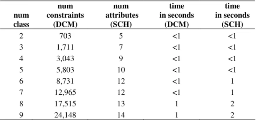
The functional measures for the first phase of the algorithm, the Disjoin Constraint Matrix (DCM), are the number of constraints and the time in seconds; for the second phase, the Set Covering Heuristic (SCH), the number of attributes and the time in seconds are taking into account. In table 1, the computational results are presented, where the locations were tested beginning with 2 classes and finishing the selected 9.
Table 1. Number constraints and computing time
num class num constraints (DCM) num attributes (SCH) time in seconds (DCM) time in seconds (SCH) 2 703 5 <1 <1 3 1,711 7 <1 <1 4 3,043 9 <1 <1 5 5,803 10 <1 <1 6 8,731 12 <1 1 7 12,965 12 <1 1 8 17,515 13 1 2 9 24,148 14 1 2
The growth of the number of constraints tends to be exponential with the number of classes (or birthplaces), while the number of attributes (or proverbs) and the computational times growth remains linear.
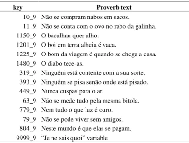
The results for the selected 9 locations (or classes), returned 14 proverbs, as the minimum information needed to identify the birthplace of the interviewee, which are presented in table 2.
Table 2. The 14 proverbs needed to differentiates the locations
key Proverb text
10_9 Não se compram nabos em sacos.
11_9 Não se conta com o ovo no rabo da galinha. 1150_9 O bacalhau quer alho.
1201_9 O boi em terra alheia é vaca.
1225_9 O bom da viagem é quando se chega a casa. 1480_9 O diabo tece-as.
319_9 Ninguém está contente com a sua sorte. 393_9 Ninguém se pisa senão onde está pisado. 449_9 Nunca cuspas para o ar.
63_9 Não se mede tudo pela mesma bitola. 779_9 Nem tudo o que luz é ouro.
79_9 Não se pode viver sem amigos. 804_9 Neste mundo é que elas se pagam. 9999_9 “Je ne sais quoi” variable
Analyzing the 14 proverbs, it sounds bittersweet, because the chosen proverbs are not the best known, nor the most beautiful, but are surely those that better differentiated the nine places.
4.2 Validation of the LAID method
To validated supervised learning problems the cross-validation is an every useful technique, which involves the partition of the sample dataset into subsamples of repeated training and testing.
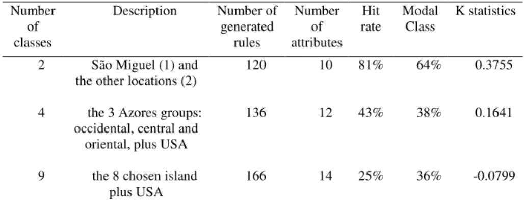
In this work, we adopt the Leave-One-Out cross-validation, which consist of removing one observation from the original sample, and then, test this observation using the resulting sample. The dataset reduction results in a dozen of attributes and a hundred of rules, as shown in table 3, for three specific classifications with 2, 4 and 9 classes.
The classification method returns for each observation the class with the minimal Hamming distance when compared to the generated rules. Following the Leave-One-Out principle, the rule that was generated by the observation will not be included.
Table 3. Number of rules, attributes and Accuracy measure Number of classes Description Number of generated rules Number of attributes Hit rate Modal Class K statistics
2 São Miguel (1) and the other locations (2)
120 10 81% 64% 0.3755
4 the 3 Azores groups: occidental, central and
oriental, plus USA
136 12 43% 38% 0.1641
9 the 8 chosen island plus USA
166 14 25% 36% -0.0799
To validate the algorithm results we are going to use the hit-rate and the k-statistics. As is well known hit-rate cannot evaluate the performance of an algorithm when different class distributions are in consideration. Hit-rate and modal class classification are calculated in table 3 where we can see that the algorithm performs well for 2 and 4 classes, compared with the modal class classification. As defined before, the hit-rate was calculated using leave-one-out procedure.
Cohen's kappa measures the agreement between the classification performances of two algorithms when both are rating the same object. A value of 1 indicates perfect agreement and a value of 0 indicates that agreement is no better than chance. The results for this algorithm, for 2 and 4 classes, is acceptable but the value for 9 classes indicates a bad classification performance, k=-0.0799. As the number of classes increases the classification procedure is increasingly difficult as the wrong classification improves probability. Off course the k-statistics includes this effect but in this case the performance degradation was bigger for the algorithm than for the random classification.
5 Conclusions
In conclusion we would like to clarify about the driver and the tool in this paper. The driver is the paremiologic study and the proposed tool is the Logical Analysis of Inconsistency Data (LAID).
This paper is part of a wider paremiologic project, based on data collected by thousands of interviews made to people from Azores, asking for the recognition of twenty-two thousand Portuguese proverbs, with the purpose of discovering the minimum information needed to guess the birthplace island of an interviewee. In the sample were include mobile persons, i.e., persons that have lived in several locations at least 5 years in each other. The mobile persons introduce inconsistency (or class noise) to the classic classification techniques, so we adopt for a Rough set approach.
A comparison of Rough sets as LAD are presented and combined in the proposed Logical Analysis of Inconsistent Data (LAID). This new technique includes the inconsistency tolerance and the multiplicity of classes of the Rough sets, and the efficiency and attributes cost optimization of the LAD. Rough sets do not exclude or correct the inconsistencies of the data, on the other hand LAID does not exclude but correct the inconsistencies by adding the “je ne sais quoi” variables. The integration of the two approaches is so tight that LAID can be seen as a Rough set extension.
The paremiologic case study uses a dataset with 240 interviewees (observations), 180 proverbs (attributes) and 15,300 records in the table of knowledge of person-proverb, classified in 9 locations (or classes). The LAID algorithm reduces the number of attributes from 180 to a mere 14 proverbs in a few seconds.
Finally, we believe that an important bridge was established between Rough sets and the Logical Analysis of data with the LAID method, although the goal of identifying an interviewee based on his knowledge of proverbs is far from being achieved.
In future works, we plan to improve the performance measures. Another very promising issue in the Rough set theory is the Dominance-based Rough set [4] which involves attributes with nominal scales and ordinal scales.
References
[1] Boros, E., P.L. Hammer, T. Ibaraki, A. Kogan, E. Mayoraz, and I. Muchnik, An Implementation of Logical Analysis of Data. IEEE Transactions on Knowledge and Data Engineering, 12(2), pp. 292-306, March/April 2000.
[2] Chvatal, V., A greedy heuristic for the set-covering problem. Math. Oper. Res., 4, pp. 233–235, 1979.
[3] Crama, Y., P. L. Hammer, and T. Ibaraki, Cause-efect relationships and partially defined boolean functions. Annals of Operations Research, 16, pp. 299-326, 1988.
[4] Greco, S. , B. Matarazzo, R. Slowinski, J. Stefanowski, An Algorithm for Introduction of Decision Rules Consistent with the Dominance Principle, In: W. Ziarko, Y. Yao (eds.) RSCTC 2000, LNCS (LNAI), 2005, pp. 304-313, Springer Heidelberg, 2001.
[5] Pawlak, Z., Rough sets, International Journal of Computer and Information Science, 11: pp. 341–356, 1982.
[6] Pawlak, Z., Rough Sets: Theoretical Aspects of Reasoning about Data, Kluwer Academic Publishers, Boston, 1991.
[7] Yao, Y. Y., Neighborhood Systems and Approximate Retrieval, Information Sciences, 176, pp. 3431-3452, 2007.