Experimentation with radio environment maps for resources optimisation in dense wireless scenarios

Experimentation with Radio Environment Maps for Resources Optimisation in Dense

Wireless Scenarios

Rog´erio Pais Dion´ısio

Avenida do Empres´ario, S/N 6000-767 Castelo Branco, Portugal

Email: [email protected]

Tiago Ferreira Alves, Jorge Miguel Afonso Ribeiro

Centro de Empresas Inovadoras Avenida do Empres´ario, n.o₁

6000-767 Castelo Branco, Portugal

Email: (talves,jribeiro)@allbesmart.pt

Abstract—The rapidly increasing popularity of WiFi has created unprecedent levels of congestion in the unlicensed frequency bands, especially in densely populated urban areas. This results mainly because of the uncoordinated operation and the unman-aged interference between WiFi access points. Recently, Radio Environment Maps (REM) have been suggested as a support for coordination strategies that optimize the overall WiFi network performance. Despite some theoretical work done in this area, there are no clear experimental evidences of the benefit brought by WiFi coordination. In this context, the main objective of this experiment is to assess the benefit of a coordinated management of radio resources in dense WiFi networks using REMs for indoor scenarios. This experiment has used the w-iLab.t test environment provided by iMINDS, a cognitive-radio testbed for remote experimentation. It was shown that REMs are capable of detecting the presence of interfering links on the network (co-channel or adjacent channel interference), and a suitable coordination strategy can use this information to reconfigure Access Points (AP) channel assignment and reestablish the client connection. The coordination strategy almost double the capacity of a WiFi link under strong co–channel interference, from 6.8 Mbps to 11.8 Mbps, increasing the aggregate throughput of the network from 58.7 Mbps to 71.5 Mbps. However, this gain comes with the cost of a relatively high density network of spectrum sensors (12 sensors for an area of 60 × 20 m), increasing the cost of deployment.

Keywords–Radio Environment Map; Radio Test-bed; Radio Resource Management; Experimentation.

I. INTRODUCTION

During the last fifteen years, the WiFi technology, as a last mile access to Internet, has experienced global explo-sion. Nowadays, the WiFi networks carry more traffic to and from end-users terminals (PCs, tablets, and smartphones) than Ethernet and cellular networks combined. The success of this technology is owed to its introduction in unlicensed spectrum (ISM bands), which has furthermore allowed un-precedented innovation in the wireless technology. However, as the penetration of WiFi continues, the unlicensed bands are becoming overcrowded. Unpredictable user-deployed hot spots (smartphone) are a new source of interference and instability that can undermine the network performance. Moreover, many Internet of Things (IoT) devices also share the unlicensed spectrum with WiFi, which further increases the problem scale. In fact, interference is a limit factor of WiFi densification; this

is a result mainly because of the uncoordinated operation and the unmanaged interference between the WiFi Access Points (AP). In WiFi, each Access Point can only access locally available sensing information within single cell coverage. It cannot access global knowledge on a multi-AP network and the deployment environment, leading to a sub-optimal network configuration.

In this context, the design of the WiFi networks is complex because of the high-density of users and significant variability of capacity requirements that can be strongly dependent on location and time. The variability of the capacity demand can be faced by deploying a dynamic network infrastructure, in which WiFi access points can be switched on and off, can work on different bands, and can tune their coverage range according to the network status and QoS requirements.

Several research works have claimed that a coordinated ap-proach of the Radio Resource Management (RRM) of channel frequency and power can increase the performance of WiFi networks in dense deployment scenarios [1], and have recently demonstrated the potential economic value of WiFi coordina-tion in dense indoor Experiments [2]. Other research work claims that an important input for interference management and coordination strategies is the Radio Environment Map (REM) of the target coverage area. The REM is a dataset of spectrum occupancy and interference levels computed based on raw spectrum measurements, propagation modelling and spatial interpolation algorithms [3]. RRM algorithms can use REMs to optimize the overall network performance. In spite of several theoretical studies on the coordinated management of WiFi networks [1], there is no experimental evidences of the benefits promised by the academic or industrial research studies.

The main objective of this experiment is to assess the benefit of a coordinated approach in dense WiFi networks that make use of realistic Radio Environment Maps, using an implementation-oriented approach in a wireless testbed environment. An important performance metric is the gain in terms of average throughput, comparing the coordinated approaches with the legacy uncoordinated approach. In partic-ular, we are interested in measuring the average capacity gain, when using market available and low cost spectrum sensors in very dense indoor scenarios. The results of this experiment are very useful from a business perspective and industrial

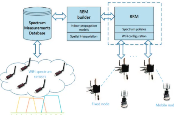
Figure 1. Generic Setup diagram for the experiment.

research, in order to realize if the actual coordination gain is sufficient enough to justify the investment in the sensing and the signalling infrastructure needed to implement a WiFi coordination scheme in realistic scenarios [3].

This paper is organised in four sections. The first section introduces the background and describes the motivation of the work. In Section II, we describe the testbed and define the setup environment of the experiments. The third section presents the experimental results with different measurements. Conclusions and future work are drawn in Section IV.

II. SETUP OF THEEXPERIMENT

This section defines and describes in detail the setup environment of the experiment.

A. Setup architecture

The setup diagram of the demonstrator, depicted in Fig-ure 1, encompasses four major components, as briefly ex-plained in the following:

• A network of spectrum sensors (energy detectors) that report spectrum measurements to a database. • A REM builder module that computes the radio

en-vironmental maps based on measurements stored in the spectrum database, the positions/configurations of radio transmitters (AP), indoor propagation models and spatial interpolation algorithms.

• The RRM that optimizes the overall WiFi network in terms of channel and power allocation based on the REM.

• WiFi APs that receive the configuration settings and reports performance metrics to the RRM module.

B. Testbed and resources allocation

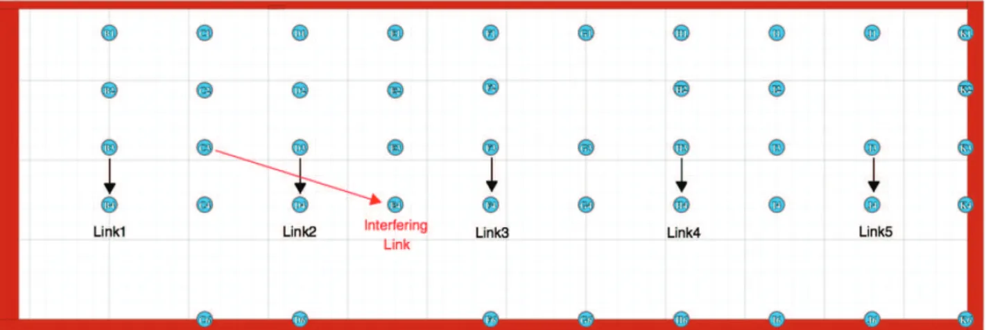
All experiments took place in a shielded environment in the W-iLab.t testbed (Ghent – Belgium). The nodes are installed in an open room (66 m by 21 m) in a grid configuration. Figure 2 shows the testing area and the locations of the nodes, represented by blue numbered circles. Each node has one embedded PC (ZOTAC) with two wireless IEEE 802.11 a/b/g/n cards (Spartklan WPEA–110N/E/11n), a spectrum sensor (Wi-Spy USB spectrum analyzer), one Gigabit LAN,

and also a Bluetooth USB 2.0 Interface and a ZigBee sensor node.

We have selected 5 equidistant links in a Client – Server configuration, represented by a black arrow in Figure 2. The distance between adjacent links is 12 m, and for each link, the distance between the client node and the AP node is 3.6 m. The red arrow represents the interfering link, with a separation of 12.53 m between nodes.

Besides the available WiFi hardware, the testbed offers several software tools to setup, control and gather radio measurements. We used the java-based framework jFed [4] to configure the testbed nodes. jFed is also used to activate nodes, install the Operating System, and SSH into the nodes. OMF6 [5] controls all the experiments, using scripts written with OMF Experiment Description Language (OEDL) [6], which is based on the Ruby programming language. The experiment description with OMF6 is structured in two main steps:

1) First, we declare the resources to be used in the experiment, such as applications, nodes, and related configurations, such as Wi-Fi channels and transmit-ted power;

2) In the second step, we define the events that triggers the experiment’s execution, and the tasks to be exe-cuted.

The Iperf traffic generator tool [7] generates data for each link using a client-server configuration for each link. All links parameters are recorded during 100 seconds for all experiments. This ensures that the radio signals for the links under test are on the air and stable. The measurements data are extracted during the experiment using OML [8]. OML is a stand-alone tool that parses and reports all the measurements to a database (SQLite3 or PostgreSQL) installed on the experiment controller server of the testbed.

C. Radio Environment Map builder

The REM is a dataset of spectrum occupancy computed based on raw spectrum measurements, propagation modelling and spatial interpolation algorithms.

There are several methods to compute REMs available on the literature, with different interpolation approaches and based on space and time spectrum measurements. One of the most commonly used methods is the Inverse Distance Weighted Interpolation (IDW) [3]. Despite the ”bull’s eyes” effect, this method is relatively fast and efficient, and present good properties for smoothing REM. In order to decrease the sensitiveness to outlier measurements, we have implemented a modified version of IDW method, which calculates the interpolated values using only the nearest neighbour’s points. In order to compute the REM, the exact position of each radio node on the w-iLab.t testbed area is defined as shown in Figure 2. REMs are computed using Matlab to facilitate the integration with the RRM algorithms, also implemented in Matlab.

D. RRM coordinating strategies

The RRM optimizes the overall WiFi network configu-ration in terms of channel, and power allocation based on the information provided by the REM. The adopted RRM strategies during the experiments are the following [1]:

Figure 2. W-iLab.t testbed environment: Distance between AP and client is 3.6m for Links 1, 2, 3, 4 and 5, and 12.53 m for the Interfering Link.

• Strategy 1: Allocate the WiFi links to disjoint, non-overlapping bands and use minimum possible transmit power for each WiFi link;

• Strategy 2: Optimize the transmit power of multiple WiFi links, when interference is detected.

III. EXPERIMENTAL MEASUREMENTS AND RESULTS

After describing the setup architecture and the testbed resources, we will explain the experimental measurement cam-paigns. Each set of measurement aims at studying the influence of measurable interference characteristics on the throughput of the WiFi network under study. The process was structured in four steps:

1) Spectrum measurements from the spectrum sensors in all WiFi frequency channels;

2) Compute the REMs based on spectrum measurements and IDW algorithm;

3) Measure and record the throughput of the radio links; 4) Apply the coordination strategy, e.g., reconfigure the channel allocation or the transmitted power of each APs.

A. Estimation of the path-loss propagation model

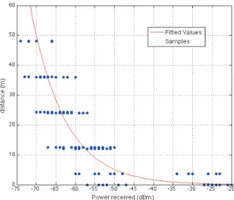
Having a suitable propagation model is a key element to build good REMs, therefore before running the experiments, we have measured the path loss between the clients and the APs in the w-iLab.t test environment to estimate the propagation model parameters. Since the majority of the nodes are in Line–of–Sight (LoS) and relatively closed to each other, as shown in Figure 2, we have considered a Free Space Path Loss (FSPL) model:

L= n (10log10(d) + 10log10(f )) + 32.45 (dB) (1)

Where L is the path loss in dB, d is the distance in meters, f is the frequency in GHz and n is the path loss exponent, which is 2 in the FSPL model. The path-loss measurement process was implemented as follows:

1) Setup one node as an AP with 5 dBm transmit power (PT x) on WiFi Channel 1 (f = 2.412 GHz), and all

the other nodes as clients.

2) For each client:

• Measure the Received Signal Strength Indica-tion (RSSI) of the AP, denoted as PRx.

• Measure the distance d between the client and the AP.

3) Setup a different node as AP and the remaining nodes as clients.

4) Repeat steps 1), 2) and 3).

The blue dots on Figure 3 represent the results of the measurement campaign.

Considering Friis transmission equation, L= PT x(dBm)−

PRx(dBm), combined with (1), we compute an estimate of the

path loss exponent n [9],

PT x− PRx= n (10log10(d) + 10log10(f )) + 32.45

⇔

n= PT x− PRx− 32.45 10log10(d) + 10log10(f )

(2)

Using (2) with the Fitting Toolbox provided by Matlab and the measured RSSI (PRx), the value of n was found to

be2.097, with a 95% confidence bounds [2.084, 2.109]. This experimentally determined value corresponds to what we are expecting for a LoS scenario. The red curve in Figure 3 shows the result of the fitting process.

Appropriate AP power levels are essential to maintaining a coverage area, not only to ensure correct (not maximum) amount of power covering an area, but also to ensure that excessive power is not used, which would add unnecessary interference to the radiating area. Transmitted power can be minimised to reduce interference among the APs.

Considering a typical baseline signal strength of -65 dBm for the WiFi received signals coming from adjacent cells, using (1) and n = 2.097, we have computed the optimal transmit power as a function of the distance, as depicted in Figure 4. This study is important to setup the initial APs transmit power to ensure a suitable cell coverage. Considering that 12 m is the separation between adjacent WiFi cells in the experiment set-up (Figure 2), the APs transmit power are set at 0 dBm, unless otherwise noted in the following experiments.

Figure 3. RSSI measurement campaign (blue dots) and corresponding fitting curve (red line).

Figure 4. Transmit power as a function of the distance, for -65 dBm received power baseline.

B. Measurement 1: Assessment of the channel distribution influence on the throughput

The aim of this experiment is to assess the influence of channel distribution on the throughput, and verify the worst-case reference scenario in terms of intra–network co-channel interference, e.g., when all APs assigned to the same channel ( Channel 1 – 2.412 GHz).

The average values of the measured throughput for each link and the aggregated throughput of the WiFi network are shown in Table I. As expected, the low values of link’s throughput are due to the strong co-channel interference that limits the overall performance of the network. Note that this is a worst-case reference scenario in terms of co-channel

interference.

TABLE I. THROUGHPUT RESULTS FORMEASUREMENT1. Throughput Measurement 1 Channel Number (Mbps)

PT x= 0dBm Link 1 1 5.25 Link 2 1 4.02 Link 3 1 3.93 Link 4 1 3.86 Link 5 1 5.28 Aggregated Throughput (Mbps) 22.34

C. Measurement 2: Considering no-overlapping channels as-signment – baseline scenario

With this experiment, all APs are configured with non-overlapping channels: Channel 1 (2.412 GHz), Channel 6 (2.437 GHz) and Channel 11 (2.462 GHz). The measured throughput presented in Table II clearly shows the advantage of using non-overlapping channels in the WiFi planning. With a transmitted power set to 0 dBm on each APs, the measured aggregated throughput is 71.50 Mbps, i.e., more than three times higher than the value in Measurement 1 (22.34 Mbps). However, if the transmitted power PT xis increased to 5 dBm,

the aggregate throughput decreases to 66.05 Mbps, because of the higher co-channel interference between Link 1 and Link 4, and between Link 2 and Link 5. Note that according to Figure 4, with 5 dBm, the APs have 22 m coverage radius.This channel configuration is the baseline for the following mea-surements.

D. Measurement 3: Channel reallocation triggered by co-channel interference

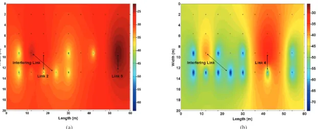
The setup for Measurement 3 has the same non-overlapping channels allocation as in Measurement 2, with an additional in-terference Link active at Channel 11, placed next to Link 2, as depicted in Figure 2. Three different interference power levels (PI) were applied during the experiment{0, 7, 15}(dBm). The

computed REMs at channel 11 for different interference link’s power are shown in Figure 5(a). The color gradient represents the computed power in dBm for a particular channel at location (x, y). The location of the nodes is added as an additional layer (black circles). The yellow dots are due the ”bull’s eye” effect typical of the IDW interpolation algorithm and should be discarded. It can be seen that by observing the REMs, we can detect not only Link 2 and Link 5, but also the extra radio activity coming from the interfering link. Note that the detection of this interfering link will trigger the coordination strategy in the WiFi network.

The results from Table III shows an overall network throughput decrease, compared with the results from Measure-ment 2, mainly due to the interference from the interfering link on Link 2 and Link 5. However, the results indicate that the variation on the power level of the interferer doesn’t have a strong impact on the aggregate throughput.

From the REM information, the coordination strategy re-allocates the WiFi channels among the APs, in order to avoid strong co-channel interference. The REM for Channel 11, depicted in Figure 5(b), shows a clear spatial separation between the interference source and Link 4.

(a) (b)

Figure 5. Measurement 3. (a): REMs with Link 2, Link 5 and Interferer Link at Channel 11 with 0 dBm; (b): REMs with Link 4 and Interferer Link at Channel 11 with 0 dBm. Color bar in dBm.

TABLE II. THROUGHPUT RESULTS FORMEASUREMENT2. Throughput Throughput Measurement 2 Channel Number (Mbps) (Mbps)

PT x= 0dBm PT x= 5dBm Link 1 1 13.27 12.16 Link 2 11 11.76 10.50 Link 3 6 21.54 21.56 Link 4 1 12.57 11.18 Link 5 11 12.36 10.65 Aggregated Throughput (Mbps) 71.50 66.05

TABLE III. THROUGHPUT RESULTS FORMEASUREMENT3. Throughput Throughput Throughput

Measurement 3 Channel (Mbps) (Mbps) (Mbps) Number PI=0dBm PI=7dBm PI=15dBm Before RRM strategy Link 1 1 12.12 12.30 12.3 Link 2 11 6.80 7.08 6.98 Link 3 6 21.59 21.63 21.61 Link 4 1 11.27 11.23 11.07 Link 5 11 6.88 6.83 6.75 Aggregated Throughput (Mbps) 58.67 58.96 58.70 After RRM strategy Link 1 6 13.27 13.12 13.10 Link 2 1 11.76 11.62 11.56 Link 3 6 21.53 21.55 21.61 Link 4 11 12.57 12.73 2.70 Link 5 1 12.37 12.41 12.40 Aggregated Throughput (Mbps) 71.47 71.43 71.38

Table III show a significant throughput increase from 58 Mbps to 71 Mbps thanks to the coordination strategy. The aggregate throughput is now close to the values obtained with Measurement 2, i.e., without any interference Link. Once again, the results indicate that the variation on the power level of the interferer doesn’t have a strong impact on the aggregated throughput.

E. Measurement 4: Channel reallocation triggered by adja-cent channel interference

With this experiment, we want to understand how the WiFi network is affected by strong adjacent channel interference and

TABLE IV. WEIGHTING FACTOR ACCORDING TO THE FREQUENCY SPACING BETWEEN CHANNELS.

n Frequency Spacing Weight

(MHz) (dB) 1 5 0 2 10 -10 3 15 -19.5 4 20 -28 5 25 36.5

how effective is the coordination strategy under such circum-stances. The interfering link is set to operate on Channel 10, while Link 2 uses Channel 11. In the case of adjacent channel interference, the REM generated for channel X has to take into account the power received from adjacent channels X±n ∈ N, weighted according to the spectral mask of the filter present at the WiFi receiver [10]. The weighting factors of the transmit mask are listed in Table IV. Note that each WiFi channel is 22 MHz wide, but the channel separation is only 5 MHz. As an example, the power of the 4th

adjacent-channel should be reduced by 28 dB to be correctly used in the computation of the REM.

The results from Table V show an overall network through-put decrease, compared with the results obtained from Mea-surements 3 and 4. This result shows that the first adjacent-channel interference leads to a higher throughput degradation than a co-channel interference (no–interference: 71.5 Mbps, co–channel interference: 58.6 Mbps and adjacent–channel in-terference: 56.7 Mbps). Once again, the results also indicate that the variation on the power level of the interferer doesn’t have a strong impact on the aggregate throughput.

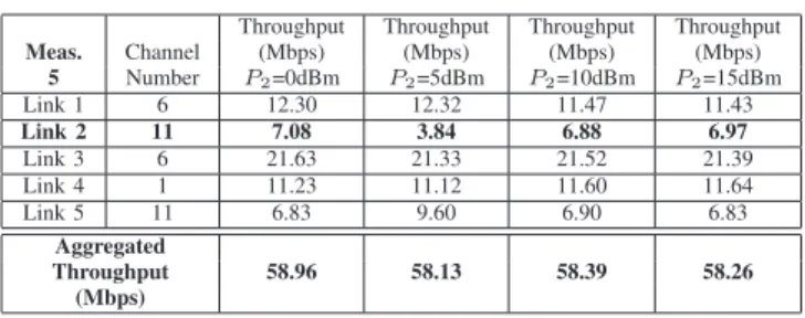
F. Measurement 5: Automatic power control to overcome co-channel interference

The aim of this experiment is to understand if automatic power control is a good strategy to overcome co-channel interference. The setup of the network under test has five links using non-overlapping channels, with an additional co– channel interference link in Channel 11. The RRM strategy in this experiment keeps the same channel assignment of each

link and increases the power of the victim link (Link 2). The transmitted power increases in steps of 5 dB, from 0 to 15 dBm. The remaining APs of the network under test remains at 0 dBm, and the interfering link is set to transmit 5 dBm in Channel 11. The measured throughput is listed in Table VI.

The results suggest that, despite the increase of transmitted power on Link 2, the overall throughput remains low and approximately constant (roughly 58 Mbps), therefore, power increase alone does not overcome the degradation caused by strong co-channel interference. The WiFi coordination strategy investigated in Measurement 3 is much more effective, leading to an aggregated throughput of 71 Mbps.

IV. CONCLUSION

This paper presented the testing of WiFi coordination strategies that exploits information from Radio Environment Maps, based upon five exploratory measurement campaigns in a pseudo-shielded testbed environment.

The overall performance of the WiFi network depends on a smart channel allocation. As an example, for the network under test, we’ve got an aggregated throughput of 22.3 Mbps in a full co-channel interference scenario and 71.5 Mbps using a configuration of non overlapping channels. It was shown that based on the observation of REMs, it is possible to detect the presence of interfering links (co-channel and first adjacent channel). First adjacent-channel interference leads to a higher throughput degradation than a co-channel interference with the same power level (no-interference: 71.5 Mbps, co-channel interference: 58.6 Mbps and adjacent-co-channel interfer-ence: 56.7 Mbps). The coordination strategy that automatically reallocates WiFi channels to avoid channel overlapping is very beneficial (e.g., the aggregated throughput goes from 58.7 Mbps to 71.5 Mbps, the link under interference goes from 6.8 Mbps to 11.8 Mbps). however, In case of strong co-channel interference, the strategy of automatically increase the power level of the victim link, when keeping the same channel allocation, does not bring any gain in terms of measured throughput.

For the RRM to be efective, 12 sensor nodes (energy detectors) were needed for an area of60 m × 20m, to create a REM with enough spatial resolution. The additional hardware required for spectrum sensing, inter–cell signalling and REM building may increase the investment by 50 %, when compared to an uncoordinated WiFi network. However, by implementing an coordinated management of radio resources, the overall throughput in WiFi network was increased more than 200 %, even in the presence of interfering links.

Future research on this work includes testing of the proposed setup architecture in the WiFi 5 GHz band, with

TABLE V. THROUGHPUT RESULTS FORMEASUREMENT4AFTER THE COORDINATION STRATEGY.

Throughput Throughput Throughput

Measurement 4 Channel (Mbps) (Mbps) (Mbps) Number PI=0dBm PI=7dBm PI=15dBm Link 1 6 8.12 8.14 8.16 Link 2 1 7.72 7.75 7.76 Link 3 6 21.53 21.51 21.55 Link 4 11 12.08 11.97 12.2 Link 5 1 11.82 11.06 11.16 Aggregated Throughput (Mbps) 61.13 60.43 60.83

TABLE VI. THROUGHPUT RESULTS FORMEASUREMENT5AFTER AUTOMATIC POWER CONTROL.

Throughput Throughput Throughput Throughput

Meas. Channel (Mbps) (Mbps) (Mbps) (Mbps) 5 Number P₂=0dBm P₂=5dBm P₂=10dBm P₂=15dBm Link 1 6 12.30 12.32 11.47 11.43 Link 2 11 7.08 3.84 6.88 6.97 Link 3 6 21.63 21.33 21.52 21.39 Link 4 1 11.23 11.12 11.60 11.64 Link 5 11 6.83 9.60 6.90 6.83 Aggregated Throughput 58.96 58.13 58.39 58.26 (Mbps)

other types of environments, including outdoor scenarios (e.g., public zones with WiFi access).

ACKNOWLEDGMENT

The research and development leading to these results has received funding from the European Union’s Seventh Pro-gramme for research, technological development and demon-stration under grant agreement N.o _{612050 (FLEX) and the}

Horizon 2020 Programme under grant agreement N.o ₆₄₅₂₇₄

(WiSHFUL)

REFERENCES

[1] L. P. Qian, Y. J. Zhang, and J. Huang, “Mapel: Achieving global optimality for a non-convex wireless power control problem,” IEEE Transactions on Wireless Communications, vol. 8, no. 3, March 2009, pp. 1553–1563.

[2] D. H. Kang, “Interference Coordination for Low-cost Indoor Wireless Systems in Shared Spectrum,” Ph.D. dissertation, KTH, School of Information and Communication Technology (ICT), Communication Systems, CoS, 2014.

[3] M. Pesko, T. Jarvonic, A. Kosir, M. Stular, and M. Mohorcic, “Radio Environment Maps: The Survey of Construction Methods,” KSII Trans-actions on Internet and Information Systems, vol. 8, no. 11, November 2014, pp. 3789–3809.

[4] iMinds. jFed – Java-based framework for testbed federation. [Online]. Available: http://jfed.iminds.be [retrieved: January, 2017]

[5] OMF–6. [Online]. Available:

https://mytestbed.net/projects/omf6/wiki/Wiki [retrieved: January, 2017]

[6] OEDL – OMF Experiment Description Language. [Online]. Available: https://omf.mytestbed.net/projects/omf6/wiki/OEDLOMF6 [retrieved: January, 2017]

[7] Iperf, The TCP/UDP bandwidth measurement tool. [Online]. Available: http://iperf.fr/ [retrieved: January, 2017]

[8] OML. [Online]. Available: https://oml.mytestbed.net/projects/oml/wiki/, [retrieved: January, 2017]

[9] A. Goldsmith, Wireless Communications. Cambridge University Press, 2005.

[10] E. G. Villegas, E. Lopez-Aguilera, R. Vidal, and J. Paradells, “Effect of adjacent-channel interference in ieee 802.11 wlans,” in 2007 2nd Inter-national Conference on Cognitive Radio Oriented Wireless Networks and Communications, Aug 2007, pp. 118–125.