Study of Perovskite Quantum Dots for Super-resolution Microscopy Applications

(1)

Ana Carolina Espada Antunes e Natal Meixeiro

Bachelor of Science

Study of Perovskite Quantum Dots

for Super-resolution Microscopy Applications.

Dissertation submitted in partial fulfillment of the requirements for the degree of

Master of Science in

Micro and Nanotechnology Engineering

Adviser: César António Tonicha Laia, Assistant Professor, NOVA University of Lisbon

Co-advisers: Luís Miguel Nunes Pereira, Associate Professor, NOVA University of Lisbon

Nuno Moreno, Unit Head, Instituto Gulbenkian de Ciência

Examination Committee

Chair: Professor Rodrigo Martins Rapporteur: Professor Ermelinda Freitas

(2)

(3)

Study of Perovskite Quantum Dots for Super-resolution Microscopy Applica-tions

The Faculty of Sciences and Technology and the NOVA University Lisbon have the right, perpetual and without geographical boundaries, to file and publish this dissertation through printed copies reproduced on paper or on digital form, or by any other means known or that may be invented, and to disseminate through scientific repositories and admit its copying and distribution for non-commercial, educational or research purposes, as long as credit is given to the author and editor.

This document was created using the (pdf)LA_{TEX processor, based on the “novathesis” template[1], developed at the Dep. Informática of FCT-NOVA [2].}

(4)

(5)

Acknowledgements

Em primeiro lugar gostava de agradecer à minha família, que apesar de pequena, é po-tente e poderosa. Aos meus avós, Zé e Odília, aos meus pais, Célia e Nuno, aos meus irmãos, Joana e Marcelo e à minha pequena sobrinha Matilde, esta vitória é tanto minha quanto vossa. Nem preciso de me alongar aqui sobre o quanto vocês significam para mim, vocês sabem. Aos meus avós, Jorge e Iria, que apesar já não estarem aqui comigo nesta vida, ensinaram me que o amor vai além da morte, e me guiaram ao longo do tempo. Ao meu alemão do coração, que além de meu companheiro foi um excelente professor, Paul Grey, obrigado por toda a ajuda pessoal e profissional. Jenny, Maren und Thomas Grey, dankeschön für die Unterstützung, Zuneigung und Hilfe. Margarida, Ricardo, Freitas, JP, Joana e João Ricardo, eu não seria nada sem vocês. Ao Matos e ao Renato, se vocês não fossem tão totós a minha vida seria demasiado monótona. Carolina Barros, Carolina Pires, Patrícia, Jaime, Ana e Diogo Garcia, desde sempre e para sempre. Débora, tu és uma das melhores pessoas que conhecia na tese, passaste me o teu valioso conhecimento sem nunca olhar para trás, o teu altruísmo ficará sempre guardado em mim, eu vou te visitar à Bélgica. Miguel Furtado, eu ainda hoje estaria a bater com a cabeça nos livros de mecânica quântica se não fosses tu. Asal e Jonas, o casal mais fixe de sempre. Carol Marques, Sara, Tomás, Centeno, Manu e Inês Cunha vocês são os maiores, e não pensem que se livram de mim. Adriana, obrigado por me teres ensinado a sprayar como ninguém, e por seres tão boa onda! Neusmar, cara se não fosse você eu hoje não tinha tese! Obrigado por tudo meu irmão!! Um agradecimento especial à Xana e à Sónia por me aturarem, por serem tão porreiras comigo e terem sempre uma palavra amiga.

Ao Professor César Laia, por ter aceite a proposta desta tese, e ter me ajudado a tornar a sopa de ideias malucas em algo com pés e cabeça. Por ter sido um excelente Professor me passar tanto conhecimento, desde fotoquímica a séries de televisão decentes.

Ao Professor Luís Pereira, obrigado por ter entrado nesta loucura, ter aturado os meus pânicos, ter sido arrastado para reuniões que podiam ter sido um email, mas mais importante que isso ter sido um dos melhores professores que tive. Levo a memória de um professor porreiro, que bebe cerveja com a malta mas acima disso levo um amigo.

Ao Professor Mauro Guerra, um brinde às amizades improváveis, entre alunos chatos que estão aterrorizados com a matéria, e os professores extraordinários que nos lembram das nossas qualidades/capacidades. Obrigado por todas as explicações incansáveis até eu entender a maldita mecânica quântica, ou pelo menos quase entender... Obrigado pelo apoio quando a saúde me falhou, pela motivação e por acreditar em mim.

(6)

Um sincero agradecimento à Professora Elvira e ao Professor Rodrigo, principalmente porque se não fosse o vosso trabalho árduo não teríamos as condições de trabalho que temos, de poder trabalhar num instituto de excelência e desenvolver tão bons trabalhos de tese. Além disso, um sincero obrigado, pelo apoio, a motivação e os conselhos.

Gostava ainda de agradecer aos Professores João Paulo Borges, Paula Soares, Jorge Parola, Sandra Gago, Susete Fernandes, Joana Vaz Pinto, Rita Branquinho, João Carlos Lima, Pedro Tavares, Alice Pereira e Fernando Pina.

I would like to thank the technical support of IGC’s Advanced Imaging Facility (AIF-UIC), which is supported by the national Portuguese funding ref# PPBI-POCI-01-0145-FEDER-022122, co-financed by Lisboa Regional Operational Programme (Lisboa 2020), under the Portugal 2020 Partnership Agreement, through the European Regional Devel-opment Fund (FEDER) and Fundação para a Ciência e a Tecnologia (FCT; Portugal).

The Associate Laboratory for Green Chemistry—LAQV and the research unit Glass and Ceramic for the Arts—Vicarte, which are financed by national funds from FCT/M-CTES (UID/QUI/50006/2019 and UID/EAT/00729/2019). The Portuguese FCT-MFCT/M-CTES for the financial support from PTDC/ QEQ-QIN/3007/2014, and the EC is acknowl-edged for the INFUSION project grant N. 734834 under H2020-MSCA-RISE-2016. The DecoChrom project under Grant Agreement No. 760973.dd

The European Commission under project NewFun (ERC-StG-2014, GA 640598) and BET-EU (H2020-TWINN-2015, GA 692373). This work was also supported by the FEDER funds through the COMPETE 2020 Program and the National Funds through the FCT – Portuguese Foundation for Science and Technology under the Project No. POCI-01-0145-FEDER-007688, Reference UID/CTM/50025, project PapEl, reference PTDC/CTM-NAN/5172/2014.

"I did a QuantumSTORM, what did you do?"

(7)

Abstract

Quantum Dots (QDs) are known for their remarkable optical properties, such as, high photoluminescent quantum yields (PLQY), large absorption spectra, narrow emission spectra, excellent photostability and the possibility to shift the fluorescence emission in a wide spectrum of colours through QD synthesis conditions [1–4]. When compared with conventional fluorophores, QDs show many advantages, like resistance to photobleaching, enhanced photostability and brightness [5]. In this work Iodine Perovskite Quantum Dots (CsP bI₃) were used, since this type of QDs show great photophysical properties and near-infrared (NIR) emission. Nevertheless, their structural stability and shelf life needed improvement, so a doping system based on cadmium was developed, and alterations in the synthesis were studied to fulfil the needs without causing any kind of drawback. An extensive optical, chemical and morphological characterisation was carried out to fully understand the influence of the developed particle engineering. It was proven that the doping system and synthesis modifications increase the stability of the nanocrystal, without pitfalls. Finally, different Super Resolution Microscopy techniques were used to investigate the performance of the PQDs, the possibility of using them as fluorescent dyes and a possible resolution enhancement.

Keywords: Quantum Dots; Iodine Perovskite; Photophysical properties; NIR; dSTORM; Confocal; Stability; Self Life; Doping; Super Resolution Microscopy . . .

(8)

(9)

Resumo

Quantum Dots (QDs) são conhecidos pelas suas extraordinárias propriedades ópticas,

como elevadas eficiências quanticas de fotoluminescência (PLQY), largo espectro de ab-sorvância, espectro de emissão estreito, excelente foto-estabilidade, e a possibilidade de ajustar a emissão de fluorescência num vasto espectro de cores, apenas alterando condi-ções na síntese dos mesmos [1–4]. Quando comparados com fluoroforos convencionais, QDs apresentam muitas vantagens, como resistência a fotobranqueamento ( photoblea-ching), melhor fotoestabilidade e brilho [5]. Neste trabalho foram usadosQuantum Dots

de Perovskite de Iodeto (CsP bI3), pois este tipo de QDs apresentam excelentes

proprieda-des fotofísicas e emissão no infravermelho próximo (NIR). No entanto, a sua estabilidade estrutural e validade necessitavam melhorias, dessa forma um sistema de dopagem ba-seado em cádmio foi desenvolvido, e alterações à síntese foram estudadas para acatar às necessidades, sem nunca prejudicar as suas características iniciais. Uma extensa caracte-rização óptica, química e morfológica foi feita para entender na totalidade a influência da engenharia da particula desenvolvida. Foi possível provar que a dopagem e as alterações à síntese aumentaram a estabilidade do nanocristal, sem desvantagens. Por fim, foram utilizadas diferentes técnicas de Microscopia de Super Resolução, para investigar o com-portamento dos PQDs, a usa possível utilização como marcadores fluorescentes e a sua possível contribuição para um aumento de resolução.

Palavras-chave: Quantum Dots; Perovskite Iodeto; Propriedades fotofísicas; NIR; dS-TORM; Confocal; Estabilidade; Dopagem; Microscopia de Super Resolução . . .

(10)

(11)

List of Figures

1.1 Perovskite structure, and possible combinations [15] . . . 2

1.2 Diffraction barrier imposed by the wave nature of light [17] . . . 3

1.3 dSTORM image reconstruction mechanism, based on the stacking of multiple

frames with each frame’s localisations [27, 28]. . . 4

1.4 Spectral behaviour of Organic Dyes and Quantum Dots. (a-f) Absorption and emission spectra (lines and symbols, respectively). (a-c) Representative Quantum Dots. (d-f) organic dyes. In all pictures the sizes are colour coded

(blue, gree, black, red - smaller to bigger, respectively) [29] . . . 5

3.1 a) Final product of the synthesis with different Cd percentages ((CsP b(1−x)CdxI3,

x = 0, 5, 10 and 20), redispersed in 5 ml of hexane (lower to higher percentage, from right to left); b) Same solutions from a) (in the same order) under UV

light (λexc= 360 nm). . . 14

3.2 Absorption spectra of different samples of PQDs with different Cd percentages redispersed in 5 ml of hexane. The black line represents the pristine (0% Cd) sample, red 5% Cd, blue 10% Cd and green 20% Cd. The inset graphic is a zoom of the indicated area between the wavelengths of 600 to 750 nm, to see

in detail the band gap area.. . . 15

3.3 Variation of the emission spectra of the PQDs samples (in Hexane) for differ-ent Cd percdiffer-entages (black is the non-doped (0% Cd) sample, red is 5% Cd, blue is 10% Cd and green 20% Cd; In the "old"image we have the emission spectra of samples in "new"aged one week (the same colour code from); in both measurements the excitation wavelength was 600 nm. The 20% Cd sample,

after one week it was no longer luminescent.. . . 16

3.4 Dashed line represents the emission spectra of the PQDs samples in hexane, the full line represents the absorption spectra in the band gap area (600 to 750 nm). The black lines are related to the pristine (0% Cd) sample, red 5% Cd,

blue 10% Cd and green 20% Cd.. . . 17

3.5 Results for comparison method and integrating sphere from the samples of

PQDs with different Cd percentages (CsP b_1−xCd_xI₃ x = 0; 5%; 10%; 20%), all

samples were redispersed in Hexane. The bigger difference for 0% Cd and

(14)

L i s t o f F i g u r e s

3.6 XRD peaks from the perovskite quantum dots, with different cadmium doping

quantities. . . 21

3.7 High resolution TEM images, a) pristine sample (0% Cd); b) 10% Cd; c) 20% Cd. . . 23

3.8 Confocal Microscopy from the initial tests, still during sample preparation study. . . 24

3.9 High resolution confocal image of a fungus spore, marked with PQDs. . . 25

II.1 Samples of PQDs synthesised in 4.07 and 5.07, 10 days after synthesis. With-out washing step, kept inside the centrifugation falcons in room conditions. The percentages indicated in the images represent the cadmium percentage. 41 II.2 Samples of PQDs synthesised in 4.07 and 5.07, 28 days after synthesis. With-out washing step, kept inside the centrifugation falcons in room conditions. The percentages indicated in the images represent the cadmium percentage. 42 III.1 Decay Times from the pristine sample 0% Cd and 5% Cd (CsP b1−xCdxI3x = 0; 5). . . 44

III.2 Decay Times from the sample with 10% Cd and 20% Cd (CsP b1−xCdxI3x = 0; 5). . . 45

IV.1 Schematic of the sample assembly to be used in the several microscopy tehc-niques. . . 47

V.1 Tauc plots for the band gap calculus. A) Pristine sample 0% Cd (CsP b_1−xCd_xI₃ x = 0); B) Sample with 5% Cd (CsP b1−xCdxI3x = 5).. . . 49

V.2 Tauc plots for the band gap calculus. C) Sample with 10% Cd (CsP b1−xCdxI3 x = 10); D) Sample with 20% Cd (CsP b1−xCdxI3x = 20). . . . 50

VI.1 Binding energy spectra from XPS analysis, pristine sample (0% Cd) . . . 51

VI.2 Binding energy spectra from XPS analysis, 5% Cd sample. . . 52

VII.1Dynamic Light Scattering results for PQDs. . . 55

VIII.13D vision of point spread function, obtained from a group of localisations from dSTORM.. . . 57

VIII.22D vision of point spread function, obtained from a group of localisations from dSTORM.. . . 58

VIII.3Centroid vision of the point spread function and localisation area, obtained from a group of localisations from dSTORM. . . 58

IX.1 Point spread function, obtained from one localisation with dSTORM. . . 59

(15)

L i s t o f F i g u r e s

IX.2 Centroid of the PSF and localisation area, obtained from one localisation with

(16)

(17)

List of Tables

3.1 Time-resolved photoluminescent decay times, of the PQDs samples with

dif-ferent doping percentages, redispersed in hexane.. . . 18

3.2 Summary of photo physical properties of the PQDs. . . 19

3.3 XPS element analysis for each sample, with different Cd percentages (CsP b1−xCdxI3 x = 0; 5; 10; 20). . . . 19

3.4 Theoretical quantities of each element in CsP bI3. . . 20

3.5 Binding Energy values for each element, from every sample.. . . 20

(18)

(19)

Acronyms

Ac Acceptor

AR Analytical grade Reagent

BE Binding Energy

CT Contrast

D Donor

DB Dangling Bond

DLS Dynamic Light Scattering

dSTORM direct Stochastic Optical Reconstruction Microscopy

EDS Energy Dispersive X-ray Spectroscopy

HRConfocal High Resolution Microscopy

ICP Inductive Couple Plasma Spectroscopy

MPM Multiphoton Fluorescence Microscopy

N Number of replicates

NA Numerical Aperture

NIR Near Infrared

NIRES Near Infrared Emission Saturation Nanoscopy

OA Oleic Acid

Oam Oleylamine

ODE Octadecene

PALM Photoactivated Localisation Microscopy

PLQY Photoluminescent Quantum Yield

(20)

AC R O N Y M S

PSF Point Spread Function

QD Quantum Dot

SEM Scanning Electron Microscopy

SIM Structured Illumination Microscopy

SOFI Super Resolution Fluctuation Imaging

SRM Super Resolution Microscopy

STED Stimulated Emission Depletion

TEM Transmission Electron Microscopy

UCNPs Upconversion Nanoparticles

XPS X-ray Photoelectron Spectroscopy

XRD X-Ray Diffraction

(21)

Symbols

A Absorbance

α Absorption coefficient A_R Absorption of the reference

AS Absorption of the sample

d Thickness

Dh Hydrodynamic Diameter

Eg Band gap

h Planck constant

IR Integrated area of the emission spectrum of the reference

IS Integrated area of the emission spectrum of the sample

λ Wavelength

λexc Excitation wavelength

n_R Refractive index of the reference

nS Refractive index of the sample

Φ_R Photoluminescent Quantum Yield of the reference

Φ_S Photoluminescent Quantum Yield of the sample

r Nature of the electronic transition

(22)

(23)

1 Introduction

1.1 Perovskite Quantum Dots

With the identification of quantum confinement in small nanocrystalline semiconductor inclusions inside glasses and colloids, throughout the early 80s, the Quantum Dots (QDs) concept became a hot topic and has been extensively investigated since then. At that time the theoretical calculations of energy states and wave functions were still far from what was possible to achieve practically. QDs are semiconductor nanocrystals with sizes between 1 and 10 nm, that show fluorescence very different from the traditional organic fluorophores. Unlike the electronic transitions from valence band to the conduction band, this fluorescence consists in the excitation of an electron from the valence band across the band gap to the conduction band, leaving a hole behind. The exciton (electron – hole pair) suffers quantum confinement because of the size of the nanocrystal is smaller than the exciton Bohr radius. This impacts the energy of the band gap, that normally increases as the size of the QD becomes smaller. Thus, when recombinations occurs in the QD, the emitted photon have shorter wavelengths, when compared with the bulk material [6]. Today it is possible to produce QDs in many different ways, being possible to adjust the emission wavelength using compounds from the I-VII and II-VI periodic table groups for a wide-gap QDs. And also the emission throughout the whole visible spectrum up to the near-infrared spectra range with periodic group-IV and III-V compounds, respectively [7].

The most studied type of QDs is the metal chalcogenide (e.g. CdSe, InP, PbS), where usually a core/shell arrangement is necessary to achieve high Photoluminescent Quan-tum Yields (PLQYs). Recently a new class of nanocrystals, based on the Perovskite crys-tal structure, emerged and soon their properties began to challenge and exceeding the chalcogenide QDs. Due to their outstanding optical properties, Perovskite Quantum Dots (PQDs) have been used in several different applications from LEDs, Photovoltaic cells, to one that has not been much explored, but is yet very interesting, the Super Resolution Imaging. [8–10]. If the size of these nanocrystals is reduced to a few nanometers, it is possible to achieve extremely high PLQY and colour purity (narrow emission, 10 nm for blue emitters and 40 nm for red emitters) [11]. Additionally, PQDs have high tolerance to defects, and do not require a shell passivation to retain high PLQY.

(24)

C H A P T E R 1 . I N T R O D U C T I O N

an organic cation like methylammonium (MA) or formamidinium (FA), or fully inorganic (caesium, Cs). The X is a halogen (Cl, Br or I). Fully inorganic nanocrystals usually show better stability due to the lack of volatile organics, and by consequence a higher PLQY [12,13]. Their band gap is highly tunable, depending on synthesis conditions for instance [14]. The difference between the valence and conduction band and their relative

posi-tions are constituted by octahedra, which come in the form of BX6 with corner sharing

X−throughout the crystal structure. The combination of charge density (or distribution) and structure inside the perovskite crystal are thus balanced by the organic ions [12–14]. The Perovskite structure can be seen in figure1.1.

Figure 1.1: Perovskite structure, and possible combinations [15]

1.2 Super Resolution Microscopy and its Contribution to

Science.

Optical Microscopy is a vast and well-known field of investigation, which started many years ago. It was in the 17th century that the compound microscopes first appeared in Europe, since then their development was constant and wide. Nevertheless, the use of light imposed a limit on the resolution, based on the diffraction of visible light wavefronts as these pass through the circular aperture at the rear focal plane of the objective, as it is possible to see in figure1.2. This phenomenon was described by the equation1.1of the diffraction theory of Ernst Abbe [16].

d = λ/2N A (1.1)

Where d is the radius of focus, λ is the wavelength of the light and NA is the numerical aperture of the optical system (N A = n × sin(θ)), where n is the refractive index of the imaging medium (usually air, water, glycerine or oil) and θ the aperture angle.

(25)

1 . 2 . S U P E R R E S O LU T I O N M I C R O S C O P Y A N D I T S C O N T R I B U T I O N T O S C I E N C E .

Figure 1.2: Diffraction barrier imposed by the wave nature of light [17]

To surpass this limit new microscopy techniques were developed, using a different light source and fluorescent molecules [18–20]. These techniques can be categorised into two groups: those that modulate the fluorescence spatially with patterned illumination, and those that stochastically activate individual molecules at different times [21]. The first group includes Stimulated Emission Depletion (STED) [22] and Structured Illumina-tion Microscopy (SIM) [23], while in the second group Stochastic Optical Reconstruction Microscopy (STORM) [24] and Photoactivated Localisation Microscopy (PALM) [25] can be included.

The focus of this work is on the techniques included in the second group, that allow to localise single molecules, by stochastically switching ON only a small quantity of fluorescent dyes in the viewing zone, where this random activation is induced by the photoswitching mechanism [26]. Direct Stochastic Optical Reconstruction Microscopy (dSTORM) relies on this random activation and readout of the individual fluorophores’ emissions. This is possible by transferring most fluorophores to a reversible OFF state, and then stochastically activating single molecules. If the activation probability is low enough, the activated fluorophores are spaced apart more than the resolution limit, and their localisation is determined by fittings of the point spread function (PSF) to the photon distributions. This procedure is repeated several times to reconstruct the image, by stacking the frames of each activation/localisation, as can be seen in figure1.3[27].

(26)

Figure 1.3: dSTORM image reconstruction mechanism, based on the stacking of multiple frames with each frame’s localisations [27,28].

1.3 Quantum Dots as Biological Fluorescent Markers.

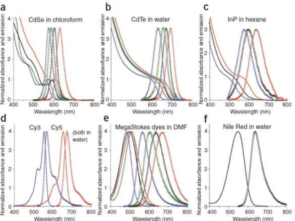
The potential of the detection and the imaging depends profoundly on the used chro-mophore and its properties such as: chemical nature, size, biocompatibility, and interac-tion between dye and biological assembly. Regarding spectroscopy, its relevant properties are: the absorption and emission bands, and for the latter, its spectral position, width and shape. Furthermore, the Stokes shift, molar absorption coefficient and PLQY. This affects the detection limit, dynamic range, reliability of the readout, and suitability for multiplex-ing [29]. In organic dyes these properties depend on the electronic transition(s) and can be tuned by complex design engineering. Most common fluorophores are resonant dyes where the emission is from an optical transition delocalised over the entire chromophore. These are characterised by being slightly structured, absorption and emission bands are often mirror of each other, small polarity dependence, high molar absorption coefficients and moderate PLQY. They usually show a poor separation between the absorption and emission spectrum, which favours the cross-talk between different chromophores, which is the contamination of the emission channel of one chromophore by the emission of another one. This behaviour can be affected by the band width and the absorption over-lapping of several chromophores.

(27)

1 . 3 . Q UA N T U M D O T S A S B I O L O G I C A L F LU O R E S C E N T M A R K E R S .

Another option are the contrast dyes that show intramolecular charge transfer transi-tions, resulting in well separated, broader structureless absorption and emission bands. However, they also show smaller molar absorption coefficients, smaller PLQY and strong polarity dependence [29]. The comparison of the absorption and emission spectra of some organic dyes and a few types of QDs can be seen in figure1.4, to better understand these properties.

Figure 1.4: Spectral behaviour of Organic Dyes and Quantum Dots. (a-f) Absorption and emission spectra (lines and symbols, respectively). (a-c) Representative Quantum Dots. (df) organic dyes. In all pictures the sizes are colour coded (blue, gree, black, red -smaller to bigger, respectively) [29]

Some of the fluorophores’ drawbacks, consist in the fact that they can only be excited optimally by a certain wavelength, which means that they need two different lasers for bleaching and reactivation [21–27,29, 30]. One fluorophore can be activated multiple times which can lead to blurring, since it can mark the structure many times during the imaging. Moreover, they show a relatively broad emission spectra, that may result in emis-sion overlap. In addition, common fluorophores show a moderate to low NIR wavelength PLQY, leading to an inconclusive localisation [30]. Since NIR light is necessary because it is less scattered and absorbed by biomolecules so it can penetrate into greater depth of the tissues, allowing an improvement of spatial resolution and diminished autofluorescence [31,32], the fluorophores start to be ineffective. Another drawback is that they cannot

(28)

fluorescent lifetime in NIR iscirca 1 ns, which is normally too short for an efficient

tem-poral discrimination of short-lived fluorescence [29, 30, 33]. Finally, fluorophores are also not suited for multicolour applications [30]. Due to all these characteristics where fluorophores show their inability to keep up with the advancements of super resolution fluorescence imaging, an alternative is required.

QDs are the leading candidate to solve some of the problems associated with the use of fluorophores. Some of the advantages of QD are: brighter fluorescence, excep-tional photostability, resistance to photobleaching, tuneable emission spectra and broad excitation and narrow emission spectra [30]. Additionally, they allow simultaneous ex-citation and detection of different colours, enabling multitracking, multi-biosensing or three-dimensional imaging. Furthermore, QDs can emit IR or NIR with high stability, thus they are highly suited for deep tissue imaging. Their inorganic nature allows their resistivity to metabolic degradation. Unlike organic fluorophores, QDs showed fluores-cence inside living cells and organisms after several weeks, with no detectable toxicity [34–39]. This enables a long-term study of the same culture of cells or organisms, which is remarkable for biology. The study and use of QDs have been growing in the past few years, some of the applications have shown:

• Mn-doped ZnSe nanocrystals’ fluorescence can be modulated with an efficiency greater than 90% through reversible excited-state absorption;

• ZnSe QDs were used to achieve a 4.4-fold increase in the resolution over the di ffrac-tion limit with the RESOLFT technique (reversible saturaffrac-tion optical fluorescence transitions) [40];

• ZnSe were also used in 4Pi microscopy were it was possible to achieve an axial resolution of 100 nm [41];

• CdSe QD were implemented to enhance spatial resolution by exploiting natural blinking or enhanced blinking with SOFI (super resolution fluctuation imaging) [42,43].

By extraction of the PSF of individual QDs (subtracting successive frames), it was pos-sible to achieve 3D super-resolution imaging [43]. Many more applications and advance-ments have been done in the biolabeling and bioimaging field, as well as in biosensing, biodetection, small molecule detection, temperature/pH/oxygen sensing and therapy [44]. Recent studies proved that it is also possible to perform 3D tracking of QDs in living cells by an automatic recognition of out-of-focus diffraction patterns [45]. But not everything has been easy with QDs, as they spend relatively short time in theoff state, decreasing the number of QDs that can be distinguished inside the point spread function. This is a limitation when applying them in STORM, it is mandatory that QDs spend greater time in the off than in the on state. However, this problem has been solved by

(29)

1 . 3 . Q UA N T U M D O T S A S B I O L O G I C A L F LU O R E S C E N T M A R K E R S .

applying the Blueing technique [21]. In the high resolution Multiphoton fluorescence microscopy (MPM) technique it is possible to obtain deeper penetration, decreased noise and reduced phototoxicity, but the technique requires spatial alignment and temporal synchronisation of high-power femtosecond switching lasers, which is impossible in the current probe technology, for the conventional MPM this is not necessary but the resolu-tion is decreased. Recently, a study showed that with a special type of QDs, upconversion nanoparticles UCNPs, it is possible to unlock a new mode of NIR emission saturation nanoscopy (NIRES) with a much lower excitation intensity than the one required in MPM dyes, enabling the use of normal MPM equipment with higher deep tissue resolution [46]. The evolving work in this field brings great advancements in many other areas, since a continuous developing of microscopy influences a great number of fields of research. With the development of new techniques and improving the present ones, it is possible to evolve other areas too, which brings great satisfaction and fulfilment. QDs are a recent technology, still unknown of their full capabilities.

By exploring new QDs like PQDs, it is possible to find a new way to improve the resolution of the present microscopy techniques, since perovskite QDs have shown re-markable brightness [47]. It is believed that the signal that reaches the camera of STORM technique is higher, and so the point spread function is more defined and constrained, enabling a more effective localisation.

(30)

(31)

2 Materials and Methods

2.1 Quantum Dots Synthesis

To synthesise the Perovskite CsP bX3quantum dots, the previously reported hot-injection

method was used [11, 48]. In this work only CsP bI₃ were synthesised and used. The reagents were used as received without any purification. caesium carbonate, Cs2CO3

(99%), oleic acid (90%); octadecene (90%); lead iodide, P bI2(99.999%); cadmium iodide,

CdI₂(99%) were purchased from Sigma Aldrich, and oleylamine (80-90%), from Acros Organics. During the course of the project a range of various cadmium (Cd) percentages were tested to understand the doping threshold and its influence in terms of photophysi-cal properties.

A study of the influence of the Cd in the structural stability was carried out, and six different concentrations were used. The pristine (control) sample without Cd, a 5% Cd, 10%, 15%, 20%, 30% and 50%, (CsP b1−xCdxI3x = 5, 10, 15, 20, 30, 50). The specific

conditions of the procedure can be seen in annexI.

2.2 Optical Characterisation

Here is described the optical characterisation of the PQDs with the different Cd percent-ages. The samples with 30% and 50% Cd were discarded and were not characterised, since the synthesis was not successful for these concentrations. For the absorption and emission spectra a 1 cm optical path quartz cell was used, containing 3 ml of a diluted so-lution of each sample, with a concentration of approximately 3.6 mg/ml. The absorption was measured using a Cary 100 UV-Visible Spectrophotometer from Agilent Technolo-gies, from 200 nm to 800 nm, with a "hexane-hexane"baseline. For emission spectra an HORIBA Spex 3 spectrofluorimeter with a photomultiplier tube detector was used. Both measurements were conducted at room temperature and the PQDs samples were dispersed in analytical grade reagent (AR) hexane. The references used were Rhodamine 6G and Nile Blue, and for their measurements both samples were dispersed in ethanol AR.

The Photoluminescent Quantum Yields (PLQY) of the PQDs was determined with two different methods. The comparison method, which is a relative method, and an

(32)

C H A P T E R 2 . M AT E R I A L S A N D M E T H O D S

absolute method, the integrating sphere. In the first method Nile Blue was chosen as a reference due to its absorption and emission spectra, this fluorescent specie exhibits the closest behaviour to the PQDs. For Nile Blue a λexc of 600 nm was used (for reference

and samples), and the results will be discussed further in this document, in chapter3. The measurement of the PLQY through the comparison method was obtained using the equation2.1[49]. Φ_S= Φ_R×IS IR ×(1 − 10 −_A_R ) (1 − 10−_A_S₎× n2_S n2_R (2.1)

WhereΦ_Sstands for the PLQY of the sample,Φ_Rstands for the PLQY of the reference.

IS is the integrated area of the emission spectrum from the sample, and IR is the one

from the reference. AS the absorption at theλexcfor the sample, andARthe one for the

reference. Finally,n_S is the refractive index of the solvent of the sample andn_Rthe one from the reference [49].

For a more absolute measurement of the fluorescence quantum yields an integrating sphere was used. In this method, an 1 cm optical path quartz cell with the same amount of sample and concentration from the comparison method was used. Three different tests were obtained, one with no sample in the sample holder, one with direct incident excitation light and one with indirect excitation light. From each test two spectra were ob-tained, the fluorescence and the scattered light. From these 6 spectra for each sample were calculated the quantum yield results. The equation used was (Ec-(1-abs)*Eb)/(La*abs

Ec − (1 − abs) × Eb

La × abs (2.2)

Where Ec stands for the area of the fluorescence of the sample with direct excitation spectrum, abs is the absorbance spectrum area of the sample, Eb is the area of the fluores-cence spectrum with out of beam excitation, La stands for the area of the scattered light of the sphere without sample spectrum.

Finally, to characterise the time decays of the PQDs, measurements of the Transient Luminescent Decays were conducted and the procedure can be found in annexIII.

2.3 Chemical Characterisation

X-ray Photoelectron Spectroscopy (XPS) was used to confirm the doping quantities, stoi-chiometry of the reaction, energy band gap and oxidation states of the compounds. The measurements were obtain with an ultra-high vacuum AXIS-Supra photoelectron spec-trometer (Kratos Analytical Ltd.,UK), equipped with a 165 mm mean radius hemispher-ical and spherhemispher-ical mirror analyzer, a monochromatic Al source, and an Argon cluster sputter gun (up to 2000 atoms) (1486.6 eV). The solutions from the different samples with different cadmium percentages (CsP b_1−xCd_xI₃x = 0; 5; 10; 20), dispersed in hexane

were drop-casted on a silicon wafer without native oxide. The hexane evaporated leaving a thin film of PQDs, that was analysed.

(33)

2 . 4 . M O R P H O L O G I C A L C H A R AC T E R I S AT I O N

The samples were studied with X-ray Diffraction (XRD). The equipment was a X’Pert PRO MPD, Multi-Purpose Diffractometer in a Theta-Theta configuration. The cadmium concentrations of 0%, 5%, 10%, 15%, 20% and 30% were analysed to study the evolution of the structure with the doping. To make this measurement, the PQDs hexane suspension was deposited via drop-casting multiple times on a silicon substrate cut at 5º (to avoid XRD background), until the mass of sample was sufficient for the measurement.

2.4 Morphological Characterisation

To study the PQDs size, Dynamic Light Scattering (DLS) was performed using a SZ-100 nanopartica series (Horiba, Lda) with a laser of 532 nm, at room temperature. The measurements were carried out for diluted PQDs suspension in hexane, with N = 16 (N, number of replicates). It was used a quartz cell, with a scattering angle of 90º. Cumulants statistics were used to measure the hydrodynamic diameter (Dh).

Transmission Electron Microscopy (TEM) was used to confirm the DLS results and to characterise the morphology of the nanocrystals. It was used a TEM HR–TEM200–SE/EDS: HR-(EF)TEM. The cadmium percentages of 0%, 10% and 15% were deposited via drop-casting on a copper mesh.

2.5 Final Application in Microscopy

In this section the final application of the PQDs, from the sample preparation to the confocal and dSTORM techniques, are shown. The resulting images can be found in chapter3.

2.5.1 Sample Preparation

The samples for confocal and dSTORM were prepared via spray casting, on a cover slit. The samples, redispersed in 25 ml of hexane, before deposition were submitted to sonica-tion for 30 minutes at 200 watts. Then 10 µl of the sample, with an average concentrasonica-tion of 0.144 mg/ml, was filtered and redispersed in 10 ml of pure hexane. After this 4 ml of this final diluted solution was loaded into the spray gun. 1 Bar of pressure and a 15 cm distance from the target were kept during the all deposition. The deposited cover slit was then placed over a microscopy slit and it was sealed with epoxy resin. A schematic of the sample can be seen in figureIV.1in annexIV.

2.5.2 Confocal Microscopy

A Leica SP5 confocal system at Instituto Gulbenkian de Ciência was used to verify the luminescent signal of the quantum dots, and to verify if it was possible to use the quantum dots in super resolution microscopy. The equipment was mounted on a Leica DM6000

(34)

C H A P T E R 2 . M AT E R I A L S A N D M E T H O D S

inverted microscope, it was user a 633 nm excitation laser, and with 3x spectral PMT detectors and the signal was read on the 645/30 channel with a Fast Filter Wheel (FFW).

2.5.3 direct Stochastic Optical Reconstruction Microscopy (dSTORM)

Images were acquired on a custom made system based on a Nikon Ti microscope body, equipped with a Hamamatsu Flash ORCA 4.0, using the a Nikon 100x 1.45 NA Oil im-mersion objective. A 642 nm Vortran Stradus 100 mW laser was used to excite the PQDs. For maximum specificity, a Chroma 640LP filter for 642 excitation was used. Images were acquired with a MicroManager microscope control software. The reconstruction algorithm used to obtain the final images was ThunderStorm, with different parameters. 2.5.4 Irradiation Tests

The sample of PQDs with 10% Cd (CsP b1−xCdxI3x = 10), redispersed in hexane, was

placed inside a 1 cm optical path quartz cell. And the sample was irradiated for 30 minutes, 1 hour and 3 hours. In the end of each irradiation time, an absorption spectra was obtained (using the same equipment described in Absorption and Emission Spectra in this chapter). For the irradiation test a Xe/Hg lamp from Newport 67005 from Oriel Instruments USA was used, with 200 W power.

(35)

3 Results and Discussion

This is the chapter where all the results from the characterisation techniques for the PQDs with different Cd percentages, and their application in SRM, presented in chapter2, are shown and analysed.

3.1 Optical Characterisation

In this section, the photophysical properties of the PQDs samples are investigated. The samples were maintained in an hexane solution, and the different percentages of Cd ((CsP b(1−x)CdxI3, x = 0, 5, 10 and 20), were compared. A comparison with the common

literature results is also established, in order to fully understand the improvement of the developed methods.

3.1.1 Absorption and Emission Spectra

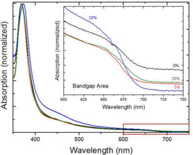
Visually it was possible to see that the emission does indeed change with different cad-mium percentages, (see figure3.1). The emission increases for 5% and 10%, and for lower or higher concentrations the emission slightly decreases. For a more accurate measure-ment absorption and emission spectra were obtained and PLQY measured. Based on the absorption spectra that can be found in the literature, it becomes evident that the absorption spectra shows an expected behaviour (see figure3.2) [50]. There is a strong absorption peak at around 370 nm, that masks the rest of the behaviour throughout the spectrum. This peak is related to another species, Cs₄P bI6, which is a rhombohedral

crystal structure [14]. In the inset graphic it is possible to see the semiconductor band gap area between 600 and 750 nm. The sample with 10% cadmium shows a slightly different behaviour, this is probably due to the reduced density of surface defects, since this percentage is the one that presents better results and higher stability over time. Less surface defects influences other properties, that are described further in this document. Besides the cadmium percentage, changes in the synthesis also induce a better tolerance to surface defects and better surface passivation. This conclusion will be discussed further in this document.

(36)

C H A P T E R 3 . R E S U LT S A N D D I S C U S S I O N

Figure 3.1: a) Final product of the synthesis with different Cd percentages ((CsP b(1−x)CdxI3, x = 0, 5, 10 and 20), redispersed in 5 ml of hexane (lower to higher

percentage, from right to left); b) Same solutions from a) (in the same order) under UV light (λexc= 360 nm).

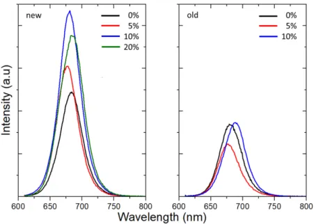
In figure3.3it is possible to analyse the emission spectra from the different cadmium percentages ((CsP b(1−x)CdxI3, x = 0, 5, 10 and 20), for an excitation wavelength (λexc) of

600 nm. It is clear that the emission peak does not change much. An important detail also is that the emission peak of the 10% Cd sample is more defined with a smaller full width at half maxima (FWHM) (table3.2) indicating a lack of surface defects, like it was mentioned before. In figure3.4, the band gap area and the emission peaks are overlapped to understand the Stokes shift of each sample. And it is clear that the Stokes shift is non-existent for all the samples. For the determination of the FWHM and the emission peak, the emission spectra were fitted by a Voigt profile equation, since the spectra are not fully Gaussian nor Lorentzian (table3.2) [51,52]. The sample for 10% Cd (CsP b1−xCdxI3x=

10%), is the one that shows a higher contribution from Lorentzian function, indicating an homogeneous broadening. The band gap was calculated based on the Tauc relation, described by the equation3.1[53,54]:

αvh = C(hv − Eg)

1

r (3.1)

Whereαis the absorption coefficient,vis the frequency,hthe Planck constant,ris the value related to the nature of the electronic transition, in this case it is a direct allowed transition, so r = 1₂, and finally theEg is the band gap. The absorption coefficient can be

calculated according to the equation:

α = 2.303A

d (3.2)

(37)

3 . 1 . O P T I C A L C H A R AC T E R I S AT I O N

Here theAstands for absorbance anddis the thickness of the used cuvette (10 mm).

The graphics for each sample with different Cd percentages, can be seen in annexV, and the determined band gap values can be found in table3.2. In most of the literature the band gap is usually referred to as being 1.73 eV, but a larger band gap is visible for higher doping percentages, peaking for the 10% Cd sample [8–10].

Figure 3.2: Absorption spectra of different samples of PQDs with different Cd percentages redispersed in 5 ml of hexane. The black line represents the pristine (0% Cd) sample, red 5% Cd, blue 10% Cd and green 20% Cd. The inset graphic is a zoom of the indicated area between the wavelengths of 600 to 750 nm, to see in detail the band gap area.

(38)

Figure 3.3: Variation of the emission spectra of the PQDs samples (in Hexane) for different Cd percentages (black is the non-doped (0% Cd) sample, red is 5% Cd, blue is 10% Cd and green 20% Cd; In the "old"image we have the emission spectra of samples in "new"aged one week (the same colour code from); in both measurements the excitation wavelength was 600 nm. The 20% Cd sample, after one week it was no longer luminescent.

(39)

3 . 1 . O P T I C A L C H A R AC T E R I S AT I O N

Figure 3.4: Dashed line represents the emission spectra of the PQDs samples in hexane, the full line represents the absorption spectra in the band gap area (600 to 750 nm). The black lines are related to the pristine (0% Cd) sample, red 5% Cd, blue 10% Cd and green 20% Cd.

3.1.2 Quantum Yield measurements

One of the most important characterisations is precisely the PLQY, being this an intrinsic property of a fluorescent specie, it is the ratio between the number of emitted photons through fluorescence, to the number of absorbed photons. As mentioned before, the PLQY was first characterised through the comparison method, using two different standards (references), but in this only the Nile Blue results were taken into account, like mentioned before. For an absolute determination of the PLQY an integrator sphere was employed, the obtained data from this method was used to confirm some of the results from the comparison method, (see in figure3.5).

The results for Nile Blue as a reference are extraordinarily high. This is an interesting result, due to the fact that the absorption of the PQDs for this wavelength (600 nm) is not high, but since it’s closer to the band gap, the photoluminescent process is more effective. Nevertheless, the Nile Blue results were considered unitary, under the experimental error.

With the results from the integrating sphere, it was possible to confirm the variation tendency of the different samples. The samples of 5% and 10% (CsP b_1−xCd_xI₃x = 5; 10)

continue to be the percentages with highest PLQY, being able to determine an approxi-mate doping threshold in terms of photoluminescence. When taking into considerations

(40)

other characteristics, further in this work it will be possible to understand that the per-centage of 10% has better results than the 5% Cd.

Figure 3.5: Results for comparison method and integrating sphere from the samples of PQDs with different Cd percentages (CsP b1−xCdxI3x = 0; 5%; 10%; 20%), all samples

were redispersed in Hexane. The bigger difference for 0% Cd and 20% is mainly due to the resolution limit of the equipment.

3.1.3 Transient Luminescent Decays

The time-resolved PL decay times of the different cadmium percentages were studied. The PL decay curves were fitted with a bi-exponential function to determine the decay times of the fast nonradiative recombinations, and the slow radiative recombinations. The results for the radiative component is on Table3.1, the shortest component is not de-tectable with this experimental setup, and is mixed with the laser scattering. The average radiative decay time is around 20.85 ns ± 1.19 ns.

Table 3.1: Time-resolved photoluminescent decay times, of the PQDs samples with di ffer-ent doping percffer-entages, redispersed in hexane.

Cd percentage 0% 5% 10% 20%

τ2 time (ns)_20.59 std dev_0.68 time (ns)_21.01 std dev_1.27 time (ns)_22.66 std dev_0.94 time (ns)_23.02 std dev_1.12

There is a slight tendency of smaller decay times for higher dopant concentration An interesting result are the decay times for 10% and 20% since for these percentages the quantum dots exhibit the best results in terms of stability, specially 10% that shows the highest PLQY. This result may confirm what was stated before, about less surface defects. Surface defects are often related to under-coordinated Pb atoms on the surface

(41)

3 . 2 . C H E M I C A L A N D S T R U C T U R A L C H A R AC T E R I S AT I O N

of the nanocrystal, serving as non-radiative recombination centers, reducing the PLQY [55]. Using cadmium as a dopant, the structure will be enriched. Also this can be once again related to the surface passivation by the surfactants, induced by the changes in the synthesis. In this case the surfactants are passivating the under-coordinated Pb atoms, increasing PLQY, lifetime and stability [55]. When compared with the literature, these decay times are lower than usual, [50,55].

In table3.2, it is possible to see the summary of the photophysical properties, for the different cadmium percentages (CsP b_1−xCdxI3x = 0; 5; 10; 20), obtained through the

characterisation accomplished during this work.

Table 3.2: Summary of photo physical properties of the PQDs.

Sample

(Cd percentage) Emission Peak (eV) FWHM (eV) Band gap (eV) PLQY (%)

0% 1.813 0.114 1.766 ± 0.165 50.6 ± 0.01

5% 1.829 0.111 1.762 ± 0.165 92.0 ± 0.01

10% 1.821 0.111 1.813 ± 0.165 92.1 ± 0.01

20% 1.813 0.121 1.791 ± 0.165 75.2 ± 0.01

3.2 Chemical And Structural Characterisation

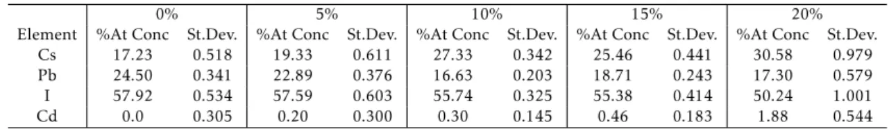
To better understand the stoichiometry and confirm the assumption made before, about the passivation of the Pb atoms, the atomic ratios of the various samples were determined using XPS, visible in table3.3. Energy Dispersive X-Ray Spectroscopy (EDS) and Induc-tive Coupled Plasma Spectroscopy (ICP) were conducted before the XPS analysis, but due to the lack of resolution and the impossibility of analysing some of the elements, the analysis were both inconclusive.

The theoretical values of the atomic concentration percentages, for the atomic ratio 1:1:3 (Cs:Pb:I) for undoped CsP bI₃can be seen in the table3.4. Based on the XPS results, it is possible to determine that for pristine sample (0%) Cs:Pb:I the ratio obtained is 0.93:0.85:3.29. For the doped samples the ratio was considered as Cs:(Pb+Cd):I, and the results are as follows: 5% 1.05:1.00:3.27, 10% 1.48:0.88:3.17, 15% 1.38:1.11:3.15 and 20% 1.66:2.48:2.85. Although there are some fluctuations, the number of Pb atoms decreased for higher doping quantities, proving that the under-coordinated Pb atoms were substituted by Cd.

Table 3.3: XPS element analysis for each sample, with different Cd percentages (CsP b1−xCdxI3x = 0; 5; 10; 20).

0% 5% 10% 15% 20%

Element %At Conc St.Dev. %At Conc St.Dev. %At Conc St.Dev. %At Conc St.Dev. %At Conc St.Dev.

Cs 17.23 0.518 19.33 0.611 27.33 0.342 25.46 0.441 30.58 0.979

Pb 24.50 0.341 22.89 0.376 16.63 0.203 18.71 0.243 17.30 0.579

I 57.92 0.534 57.59 0.603 55.74 0.325 55.38 0.414 50.24 1.001

(42)

Table 3.4: Theoretical quantities of each element in CsP bI₃.

Element Number of Atoms Mass (g) Percent composition (%)

I 3 126.91 52.82

Pb 1 207.21 28.75

Cs 1 132.91 18.44

Total 4 720.85 100

It is possible to see that the amount of lead that is leaving the structure is not on the same proportion as cadmium is entering. The amount of lead that exits is much higher, this can be due to the fact that although the ionic radius of P b2+(119 pm) is similar to the one of Cs+(95 pm), the affinity is not the same. So even though the lead is exiting the structure, the cadmium can not enter in the same rate, this is probably the reason why samples with higher percentages are more unstable [56].

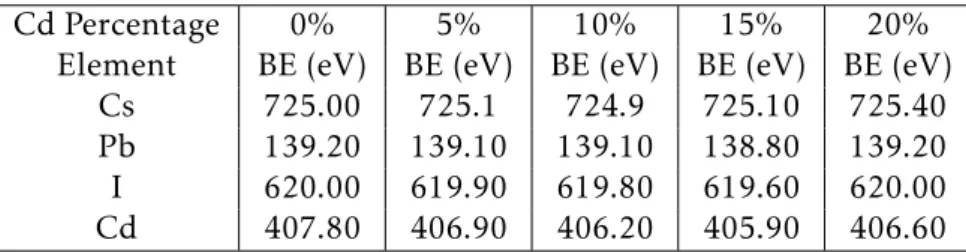
XPS technique also enabled the study of the binding energy (BE), and allowed to fully understand the chemical bonds of each element. The binding energy graphics can be found in annexVI,where a small resume of the results can be seen in table3.5.

Table 3.5: Binding Energy values for each element, from every sample.

Cd Percentage 0% 5% 10% 15% 20%

Element BE (eV) BE (eV) BE (eV) BE (eV) BE (eV)

Cs 725.00 725.1 724.9 725.10 725.40

Pb 139.20 139.10 139.10 138.80 139.20 I 620.00 619.90 619.80 619.60 620.00 Cd 407.80 406.90 406.20 405.90 406.60

Based on the literature it is possible to say that for all the samples the caesium bind-ing energy is closer to the bindbind-ing energy of CsOH, this result may confirm the possible hidroxilation, mentioned before, was successful. The binding energy of the lead is the normal binding energy of halides, which is the expected result. For iodide the binding energy of around 620 eV is the the energy correspondent of I2. And finally the energy for

cadmium around 406.50 is associated to halides [57].

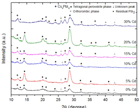
XRD was used to confirm the existence of the Perovskite structure and understand the changes induced by the cadmium doping. The obtained diffractogram can be seen in figure3.6, where the results are compared to the literature to confirm each specie present [58–60].

It is possible to identify the perovskite tetragonal phase in all samples, proving that the doping is not destroying the perovskite phase, even for percentages above 15%. It is also possible to determine the orthorombic phase, indicating that some of the perovskite structure is degrading.

(43)

3 . 3 . M O R P H O L O G I C A L C H A R AC T E R I S AT I O N

Figure 3.6: XRD peaks from the perovskite quantum dots, with different cadmium doping quantities.

In more detail, it is possible to determine the peaks at 14.10º, 20.28º, 24.7º, 28.47º, 28.81º, 32.24º, 35.42º and 41.23º that are ascribed, respectively, to the (100), (110), (211), (220), (200), (201), (211) and (220) planes of the cubic (Pm-3m) lattice, from the tetrago-nal perovskite phase. The peaks at 22.64º and 39.31º are related to the (112) and (027), which belong to a phase of the orthorhombic (Pnma) crystal. At 12.3º, 21.4º, 27.2º, 32.3º, 36.9º and 43.1º we find the XRD patterns of the Cs4P bI6phase, ascribed to (110), (300),

(214), (134), (324) and (600), respectively. Also a typical peak related to an intermediate perovskite phase is present at 24.12º. Finally, the peaks at 25.70º and 42.82º are unknown peaks, that appear with more pronunciation in the samples with higher doping quantities, indicating the presence of cadmium.

With this technique it was possible to prove the existence of perovskite phase enabling the rest of the research.

3.3 Morphological Characterisation

In order to understand the influence of the cadmium doping in the nanocrystal morphol-ogy, three different techniques were carried out: Scanning Electron Microscopy (SEM), Dynamic Light Scattering (DLS) and Transmission Electron Microscopy (TEM). SEM results had less resolution, and were substituted by TEM results, so these will not be presented in this document. DLS was conducted to study the size of the particles and with TEM the crystal shape.

(44)

3.3.1 Dynamic Light Scattering (DLS)

Using DLS, it was possible to determine an average size of the nanocrystal with its sol-vation crown. Several measurements were conducted to obtain statistical values, always from the same cadmium percentage (10%) CsP b_1−xCd_xI₃x = 10. Some of the obtained

results are presented in figureVII.1presented in annexVII.

There is a large size dispersivity, but most of the quantum dots show sizes between 18 to 29 nm. The average size is 23.9 nm ±3.0 nm. These results indicate a 2-fold big-ger average size than the usual reported in literature [12–14]. This can be attributed to the synthesis quenching time. Since the synthesis is controlled manually rather than automatic there is a large associated error. Every time the synthesis is performed the quenching times vary in few seconds or milliseconds, this is enough to create size dis-persitivity and also influence the crystal growth. But it is important to regard that the solvation crown is influencing the measurement. Therefore, through a statistic approach, TEM images were used to determined an average size for the nanocrystal.

3.3.2 Transmission Electron Microscopy (TEM)

Any kind of doping can influence the morphology of the particles, and to understand this possible change, TEM analysis was conducted on three different samples, pristine (0% Cd), 10% Cd and 20% Cd (CdP b1−xCdxI3x = 0; 10; 20). The results are shown bellow in

figure3.7.

Like mentioned before, it was used a statistical approach using the TEM images to obtain a more reliable average size value. It was used a sample population of 12 images, and in each image 30 measurements were taken. The obtained value was 17.19 ± 3.5 nm. It is possible to see that the doping is inducing a change in the PQDs. Cubic phase is predominant in pristine samples, being in accordance to what is reported in the literature ( figure a)3.7).

The presence of hexagonal shape is also visible, but in much less quantity, this can be due to a contamination, or the possibility that the hexagonal shape is not induced by the presence of cadmium, but by the lack of lead instead.

In figure b) 10% of Cd is analysed, which is the sample with best results, and the majority of the PQDs show hexagonal shape. This is an interesting result, since the shape influences a lot the stability of the quantum dot. In the image it is possible to notice that the quantum dots seem to have self assembly, like a honeycomb, but they also align in some kind of stacking, which tells us that the morphology of the nanocrystal is not a cube anymore but an hexagonal disk.

It is described in literature that dangling bonds (DBs) play a crucial role in the atomic structure of the surfaces, and surface energy [61]. Having an hexagonal disk shape instead of a cubic implicates a much different behaviour of the quantum dot. The DBs in a cubic shape nanocrystal are distributed all around the surface, but in this hexagonal shape, it

(45)

3 . 4 . M I C R O S C O P Y A P P L I C AT I O N S

is believed that the DBs are only present in the perimeter of the hexagon, since the top and bottom surfaces are poor in surface defects. This theory is not well proven in this work, but it is highly coherent with all the other results. Explaining why, in the end of the synthesis, it was not possible to redisperse the PQDs in Toluene, like described in Chapter

2. In figure c) is the sample with 20% of Cd and it is possible to see that most of the PQDs show the hexagonal disk shape, but with larger size dispersivity. Unfortunately, during this work it was never possible to comprehend if the hexagonal disk shape is originated by the presence of cadmium or the lack of lead, like it was mentioned before.

Figure 3.7: High resolution TEM images, a) pristine sample (0% Cd); b) 10% Cd; c) 20% Cd.

3.4 Microscopy Applications

In this section finally the main objective of the work is presented, which is the application of PQDs in Super Resolution Microscopy. Before that, it was necessary to develop a sample preparation that would enable to see the PQDs as separated as possible, enabling the PSF measurements. High Resolution Confocal microscopy (HRConfocal), direct Stochastic Reconstruction Microscopy (dSTORM) and Multi-Photon Absorption Microscopy (MPA) were the employed techniques. MPA was inconclusive so the results will not be presented in this work. Since the sample with 10% Cd (CsP b1−xCdxI3x = 10), was the one with the

(46)

3.4.1 Confocal Microscopy

Before testing dSTORM, a reliable proof for the possibility to use the PQDs in imaging was needed. High Resolution Confocal was the first microscopy technique to be tested. The obtained images can be seen bellow in figure3.8.

Figure 3.8: Confocal Microscopy from the initial tests, still during sample preparation study.

In the first tests, it was possible to see that the sample preparation was still not suffi-cient, several large clusters of PQDs and drying patterns were still visible. Several tests like this were conducted, until all the parameters of sample preparation were optimised. The parameters that revealed to be ideal for the sample preparation (mentioned in chap-ter2), enabled much better spatial resolution. Like the one visible in3.9, it was possible to use the PQDs as dyes in a biological structure, in this case a fungus spore. A very in-teresting detail about this sample and imaging, is that the PQDs were not functionalized biologically. The only thing connecting the PQDs and the biological material are the DBs. Due to their organic nature these bonds have a certain affinity for biological organisms. Consequently, it is possible to understand why the structure is randomly dyed. Never-theless, this is an encouraging result, since this gives us permission to continue the work in this field. Yet again, the final objective was to use dSTORM, and the results from that technique are shown next.

(47)

Figure 3.9: High resolution confocal image of a fungus spore, marked with PQDs.

3.4.2 dSTORM Applications

dSTORM technique is the highlight of this work, since the results obtained were surpris-ingly promising. dSTORM is a strong SRM technique, but to be able to use this technique, there are some main properties that the PQDs need to accomplish: strong brightness, sta-bility and blinking. The first two properties at this time of the work were already proven and improved, but the blinking property was still uncertain. This is a very important property since it completely disables the use of quantum dots in SRM in case they would not show it. In recent years it was possible to start using quantum dots in SRM due to the blueing technique [21]. But this technique is highly expensive since it involves changes in the setup from the microscope.

The blinking property of CsP bI3 PQDs is known from literature, but the results were

still poor at the time of the test [62]. It is important to keep in mind that the decay time is a different behaviour from blinking. But at the time of the first dSTORM imaging of PQDs, it was possible to see, almost instantly, that blinking of the PQDs is possible. It was possible to observe the blinking property by the human eye (and discriminate it by camera), which was a great result, since this enables the temporal separation of the localisations in each frame, which results in the spatial separation of these localisations. After several images (containing thousands of frames) were obtained and reconstructed using different parameters in the ThunderSTORM algorithm, the images with best resolu-tion were chosen and are shown in the folder "Super Resoluresolu-tion Images"in this directory

[http://bit.ly/SupInfoThesisNatal].

From these images it was possible to obtain the 3D point spread functions of single- and multi-emitters localisations, that can be found in annexesVIIIandIX. It was possible to resolve centroids closer than 64 nm, which is a very good result, yet bigger than what it is currently possible to achieve.

(48)

A possible answer for this blinking property is Auger recombination. Auger recombi-nation is a non-radiative process where at the time of an electron-hole recombirecombi-nation, the resulting energy instead of resulting in a photon, is transferred to another electron-hole pair exciting them within the same band [55]. This Auger recombination is enabled by the laser power, since under strong pumping conditions, the population of excitons is higher, which is a multiexciton interaction process.

Other possible answer for the blinking property is the existence of highly efficient quench-ing channels, known as supertraps [62]. These supertraps are quenching sites that can be empty of filled, being able or unable (respectively) to receive a charge (active or passive state) [62]. These quenchers can be described as a complex of a donor impurity (D) and an acceptor impurity (Ac). These impurities when ionized become a positively charged electron trap (D+), and a negatively charged hole trap (Ac−) respectively. The complex

D+Ac−is stable due to a Coulomb interaction, and is ready to trap both photogenerated electrons and holes. The charge carriers recombine inside the trap, and this process of trapping and recover after recombination is very short (less than 15 ns) [62]. Like this, the supertrap is rapidly available for repeating the process, enabling the blinking behaviour [62].

During the imaging of the PQDs, it was detected a behaviour that was particularly interesting. It was possible to see a partial blinking from clusters, this is, the blinking was oscillating between more than the on-off states, showing several distinct photolu-minescent intensity levels. It is possible to understand by this result, that in a cluster there are several subdomains (single PQDs), that have their own independent blinking dynamics [62]. This was possible to determine, because the emission profile changed in intensity but also in shape. Each intensity level means at least one emitter, the stronger the emission, the more emitters are on the on-state. This result is possible to see in the ".gif"file "CN-GIF-1"in this directory [http://bit.ly/SupInfoThesisNatal].

3.4.3 Irradiation tests

During the dSTORM tests, it was possible to see a decrease on the PQDs brightness. This decrease can be seen in the ".gif"files in the folder "GIF Files"in the same directory,

[http://bit.ly/SupInfoThesisNatal].

The CN-GIF-1 file was taken in the beginning of an irradiation, and CN-GIF-2 is the same area post-irradiation of several frames. In CN-GIF-3 it is possible to see a longer irradiation imaging, and a slight brightness loss during the acquisition, imaging was con-ducted under extreme conditions, with no cooling system and higher laser power.

Irradiation tests were conducted to understand the evolution of the PQDs absorption

(49)

spectra, after the irradiation. If some type of reaction is occurring, supposedly the ab-sorption spectra will be affected. It is important to keep in mind that the setup of the experiments is very distinct. The power of the laser is stronger than the lamp used for the irradiation test, another difference was the concentration of each sample. The amount of PQDs deposited over the microscope slit is infinitesimal when compared with the amount of PQDs in suspension, even if highly diluted. The results from the experiment were in-conclusive, since after the longer exposure, there was still no differences in the adsorption spectra. It is believed that the experiment setups and conditions are too different. To understand if this "bleaching"was temporary, a certain area was irradiated for 30 minutes with dSTORM (very long imaging), in the end only large clusters were still active. The area was left to "rest"without any excitation, and it was verified every 15 minutes until one hour has passed. Unfortunately, the area did not recover.

Nevertheless, a possible explanation for the "bleaching"of the PQDs is a photochemical degradation of the structure or a non-reversible charge transfer, induced by the high power laser. During this work it was not possible to determine the exact type of transfor-mation that was occurring.

(50)

(51)

4 Final Conclusions

The first main goal of this work was successful, which was the development of a sustain-able cadmium doping system for PQDs (CsP bI3 : Cd). It was possible to optimise the

synthesis for various Cd percentages CsP b1−xI3Cdx x = 0, 5, 10, 15, 20, 30, 50, and in the

end obtain stable colloidal suspensions for the percentages of 0%, 5%, 10%, 15% and 20%. After the adjustments to synthesis, centrifugation and drying, it was possible to obtain stable, dry luminescent pellets, with a much higher shelf life than reported before for similar approaches without doping. This result enables numerous applications, that were not possible up to this point.

Based on the optical characterisation, it is possible to confirm that the doping system did not affect the optical properties in a negative way. It was even possible to measure an increase in PLQY for intermediate Cd percentages, peaking for the 10 % sample.

The chemical and structural characterisation confirmed the existence of the Perovskite structure, which was a mandatory goal for this work. This proves that the developed dop-ing system does not cause any disturbance to the crystal lattice and atomic substitution took place.

Morphological characterisation (SEM and TEM) evidenced a transition from a cube to an hexagonal disk shape of the PQDs with increasing Cd percentage. Further, it was possible to determine the size via TEM, which was found to be on average 17 nm, showing the cause for quantum confinement and the observed fluorescence. Due to a shortage of time it was however not possible to further investigate this transition. Nevertheless, it is believed that this might be connected to either the direct influence of the Cd or the lack of Pb, which is being substituted by the Cd, and therefore forced out of the structure. The actual cause of this phenomenon will need further investigation.

The developed PQDs were successfully applied in super resolution microscopy, where a fungus spore was marked and observed. A possible explanation for efficient marking of the fungus spore might be connected to the presence of organic surfactant material around the PQDs, left behind by the synthesis. Fundamental properties of the PQDs, such as high brightness, stability and blinking behaviour, were confirmed, which are