Modelling and PI Control of an Irrigation Canal

MODELLING AND PI CONTROL OF AN IRRIGATION CANAL

X. Litrico

, V. Fromion

, J.-P. Baume

, M. Rijo

∗_{Cemagref, UR Irrigation, B.P. 5095, 34033 Montpellier Cedex 1, France. e-mail:}

{xavier.litrico,jean-pierre.baume}@cemagref.fr

†_{INRA, LASB, 2 place Viala, 34060 Montpellier, France. e-mail:[email protected]}

‡_{Universidade de ´Evora, Departamento de Engenharia Rural, Col´egio da Mitra, Apartado 94, 7002-554 ´Evora, Portugal.}

e-mail:[email protected]

Keywords: Open-channel system, Saint-Venant model, PI

control, Time Delay Systems, performance limitations.

Abstract

The main goal of this paper is to expose and validate a method-ology to design efficient automatic controllers for irrigation canals, based on the Saint-Venant model. This model-based methodology enables to design controllers at the design stage (when the canal is not already built). The methodology is ap-plied on an experimental canal located in Portugal. First the full nonlinear PDE model is calibrated, using a single steady-state experiment. The model is then linearized around a functioning point, in order to design linear PI controllers. Two classical control strategies are tested (local upstream control and distant downstream control) and compared on the canal. The experi-mental results shows the effectiveness of the method.

1

Introduction

The control of irrigation canals has been the subject of nu-merous scientific publications since the introduction of com-puters in the management of such large and complex systems [4]. However, only few of the proposed controllers have been effectively tested in a real situation [16]. In this paper we vali-date on a real system a model-based methodology to design PI automatic controllers for irrigation canals.

The problem of designing controllers for irrigation canals is difficult, because their management involves many different as-pects. From a control point of view, this problem is reduced to the control of water levels at some specific points in the main canal. In this case, since the water distribution is done by grav-ity offtakes, a “good” distribution is obtained by maintaining a constant water level at the offtake. In order to simplify the exposition, we will consider the case where the control speci-fication has been expressed in terms of controlling water lev-els upstream of control structures, and only consider classical control design methods (PI controllers). This is a first step val-idation for more advanced control design methods [12, 10] that will be validated in another paper [11].

From a control point of view, we want to control a nonlinear system around equilibrium points with a linear controller (typ-ically a PI). This requires a linear model of the system around the given equilibrium points.

Two main approaches can be followed to obtain a linear model in the case of irrigation canals:

1. To use identification tools [17],

2. To linearize a knowledge-based full nonlinear model, i.e. Saint-Venant equations and hydraulic structures equations (see [13] and references therein).

The cost of each approach in terms of experimental data can be summarized as follows:

1. The first approach requires to use the canal to identify the dynamics. Experiments have to cover all the required set-points of the system: a set of discharge values between maximum and minimum values, set of downstream limit conditions, set of gate openings. This has to be done on each pool of the canal, which leads to a large number of experiments, and model identifications. The system is thus represented by a large number of linear systems. 2. The second approach necessitates the data needed to

cal-ibrate a full Saint-Venant model for simulation purposes. Actually, one needs the canal geometry, and a single ex-periment in steady state (for the canal or for each pool), in order to calibrate Manning coefficients and gate discharge coefficients.

At this stage, it should be clear that the second approach is less demanding in terms of data, since the geometry is usu-ally available in most of the existing canals. Moreover, a good estimate of Manning coefficient can usually be deduced from the canal material –this is the basis of the (structural) design of irrigation canals– and even the gate discharge coefficients can be estimated from the structure geometry [8]. Therefore, once the geometry is known, this knowledge-based model can easily be obtained. This enables to have an integrated design

method for irrigation canals: the automatic control scheme can

be integrated into the structural design of irrigation canals. Since the objective is to design linear controllers, one needs

linear models. For this purpose, let us examine the implications

of both approaches:

1. In the first approach, the linear models obtained from identification can be used directly. A difficulty that arises is: How to quantify the uncertainty?

2. For the second approach, linear models have to be de-duced from Saint-Venant equations. The dynamic uncer-tainty is then directly linked to the physical parameters uncertainties (e.g. uncertainty on coefficients of Saint-Venant equations, actuator uncertainty, sensor uncertainty, etc.).

If the full nonlinear model is valid, then the second approach encompasses the first one. In fact, a linear model could be directly identified on the nonlinear simulator (see [7], [6]). However, even if Saint-Venant equations have been used by hydraulic engineers for simulation purposes, the obtention of linear models for controller design directly from the equations needs to be clarified. A first way is to consider only uniform regimes (where discharge and water depth are constant along the pool) and the associated analytical solution in the Laplace domain (see [2] [3]). In this case, how to describe the behavior in non uniform cases (i.e. the vast majority of cases)? A tenta-tive step to approximate the transfer function has been done by [16], but did not lead to an exact solution.

A second way is to use numerical schemes (e.g. Preissmann scheme) to deduce linear models (see [13], [1], [5]). In this case, how the obtained approximate model can be validated from a control point of view (in contrast to the classical valida-tion in the time-domain)?

In conclusion of this short discussion, the use of a model-based method has been largely undermined by the difficulties linked to both ways. Recent works allow to bypass these difficulties, by the obtention of a continuous linear model directly from Saint-Venant equations for any regime [9].

On this basis, we propose a complete model-based ogy to design controllers for irrigation canals. This methodol-ogy can be summarized in four successive steps:

1. Obtain the data necessary for the full nonlinear model: canal geometry, hydraulic structures description, steady state measurements (upstream discharge, upstream and downstream water levels at each structure, gate openings). 2. Calibrate the model:

– hydraulic model calibration: determine Manning and discharge coefficients using the steady state measurements,

– dynamic model calibration: model the actuators, sensors and data transmission dynamics, using either the data given the constructor, either direct identifi-cation on step response.

3. Obtain linear models based on the calibrated full nonlinear one.

4. Design controllers using the linear models. In a first ap-proximation, the actuator/sensors dynamics can be ne-glected, since they are usually very rapid compared to the canal dynamics.

The methodology is exposed and applied for simple controllers (PI). This allows to use classical design methods in order to validate the general methodology, by applying it to a real sys-tem. Once the linear models are validated, it is easy to use them to design more sophisticated controllers. Such an approach is developed in another paper [11], which examines the perfor-mance requirements attached to the control of irrigation canals. The paper is structured as follows: a brief description of the experimental canal is firstly given, then the methodology is ex-posed, and applied to this specific case. Experimental results validating the approach are finally presented and discussed.

2

Canal description

The automatic canal used in the present study is a component of the experimental facility of the Hydraulics and Canal Control Center (NuHCC) of the University of ´Evora (Portugal).

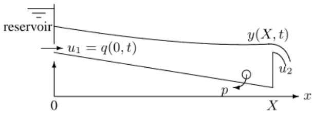
reservoir u1 = q(0, t) u2 -¾ p y(X, t) 6 -x X 0

Figure 1: Schematic representation of the experimental canal

Design The experimental canal is a trapezoidal and lined

canal, with a general cross section of bottom width 0.15 m, sides slope 1:0.15 (V:H) and depth 0.90 m. The last 7 m down-stream of canal have a rectangular cross section of 0.7 m width. The overall canal is 145.5 m long and the average longitudinal bottom slope is about 1.5 × 10−3. The design flow is 0.09 m3s−1.

A longitudinal view of the canal is schematized in figure 1.

Control devices The canal inlet is equipped with a

motor-ized flow control valve, that delivers a discharge u1. The down-stream end is controlled with a rectangular sluice gate u2 (over-shot gate).

Outlet An offtake p is located at the downstream end of the

pool, equipped with an electromagnetic flowmeter and a mo-torized butterfly valve.

Sensors A water level sensor is installed within an offline

stilling well at the downstream end of the pool, measuring the downstream water depth y. The sensor is of float and counter-weight type attached by a stainless steel tape; this tape runs over a sprocket wheel. The wheel movements are transmitted to a potentiometer that transmits to the controller the analogical input corresponding to the water surface.

3

Modelling of an irrigation canal

3.1 Hydraulic model

The Saint-Venant equations are used to model the flow in the canal. These equations are nonlinear hyperbolic partial differ-ential equations involving the average discharge Q(x, t) and the water depth Y (x, t) along one space dimension x [4]:

∂A ∂t + ∂Q ∂x = 0 (1) ∂Q ∂t + ∂Q2_/A ∂x + gA ∂Y ∂x = gA(I − Sf) (2) with A(x, t) is the wetted area [m2], Q(x, t) the discharge [m3/s] across section A, Y (x, t) the water depth [m], Sf(x, t)

the friction slope, I the bed slope and g the gravitational accel-eration [m/s2].

Two boundary conditions are necessary for this partial differ-ential system, for example Q(0, t) = Q0(t) and Q(X, t) = QX(t), where X is the length of the considered channel. The

initial conditions are given by Q(x, 0) and Y (x, 0).

The friction slope Sf is modelled with Manning-Strickler

for-mula:

Sf = Q

2_n2

A2_R4/3 (3)

with n the Manning coefficient [sm−1/3] and R the hydraulic radius [m], defined by R = A/P , where P is the wetted perimeter [m].

Hydraulic structure equation

The hydraulic structure (over shot gate) is modelled using the classical equation (free flow case):

Q = CdLv

p

2g(Y − W )3/2 ₍₄₎

with Q the discharge through the structure, Y the upstream wa-ter level, W the sill elevation and Lvthe gate width.

3.1.1 Steady flow model calibration

For a given constant upstream discharge (45 l/s), the water level and sill elevation were monitored. This steady flow period en-abled to identify the Strickler coefficient K for each pool and the discharge coefficient at each structure. The calibration lead to a discharge coefficient of 0.4 for the overshot gate and a Strickler coefficient of 60 for the canal.

3.1.2 Unsteady flow model validation

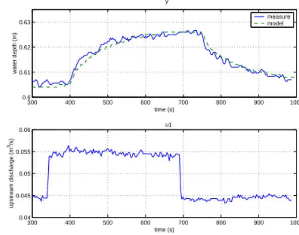
The nonlinear model calibrated in steady flow is validated in unsteady flow for different flow configurations. For simula-tion purposes, we used SIC, a computer program developed by Cemagref [14]. This mathematical model solves the full non-linear Saint-Venant equations using a finite difference scheme (Preissmann scheme). Figure 2 corresponds to the same regime

y u1 300 400 500 600 700 800 900 1000 0.6 0.61 0.62 0.63 time (s) water depth (m) measure model 300 400 500 600 700 800 900 1000 0.04 0.045 0.05 0.055 0.06 time (s) upstream discharge (m 3/s)

Figure 2: Step response around Q0 = 45 l/s, downstream boundary condition y0= 0.6 m

as the one used for the steady flow calibration. The model fits very well the data.

In figure 3, the downstream boundary condition has changed. The model is still able to accurately reproduce the level varia-tions. y u1 200 300 400 500 600 700 800 900 0.7 0.71 0.72 0.73 time (s) water depth (m) measure model 200 300 400 500 600 700 800 900 0.042 0.044 0.046 0.048 0.05 0.052 0.054 0.056 time (s) upstream discharge (m 3/s)

Figure 3: Step response around Q0 = 45 l/s, downstream boundary condition y0= 0.7 m

Many other simulations were done to validate the model, which appeared to be very accurate, even for different flow conditions. This validates the Saint-Venant model for this canal.

3.2 Control oriented model

3.2.1 Linear hydraulic model

The linear model used for control design is obtained following [9]: we consider small variations of water depth y(x, t) and discharge q(x, t) around stationary values defined by Y0(x) (m) and Q0(x) (m3/s). This leads to the linearized Saint-Venant

equations: L0∂y ∂t + ∂q ∂x = 0 (5) ∂q ∂t + 2V0 ∂q ∂x − β0q + (C 2 0− V02)L0∂y ∂x − γ0y = 0 (6) L0 is the top width for the equilibrium regime (m), V0 the average velocity (m/s) and C0 = pgA0/L0 the wave celerity (m/s). Moreover, one has γ0 = V2 0 ∂L∂x0 + gL0 £ (1 + κ)I − (1 + κ − F2 0(κ − 2))∂Y∂x0 ¤ , β0 = −2g_V 0 ¡ I −∂Y0 ∂x ¢ and κ = 7₃ − 4S0 3L0P0 ∂P0

∂Y . F0 is the Froude

number F0 = V_C0₀. A transfer matrix linear model that can be used for control purposes is obtained using Laplace transform and a specific numerical method [9].

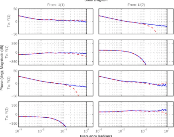
As a linearized model can be obtained from the computer program SIC, we compare the continuous time linear model with the discrete time model obtained with the finite difference scheme [13] (see figure 4). It is clear that the frequency domain responses of the models are very close up to a decade below the Nyquist frequency.

Bode Diagram

Frequency (rad/sec)

Phase (deg); Magnitude (dB)

−50 0 50 From: U(1) To: Y(1) −360 0 360 To: Y(1) −50 0 50 To: Y(2) 10−3 10−2 10−1 100 −360 0 360 To: Y(2) From: U(2) 10−3 10−2 10−1 100

Figure 4: Bode plots of the continuous model (—) and of the finite difference model (– –), for Q = 0.045 m3/s, YX = 0.6

m.

This model needs to be completed in our case with a model of the actuators and sensors dynamics. The equations describing hydraulic structures interactions with the flow are linearized and added to the model. The hydraulic structure (overshot gate) is modelled using the linearized equation:

q(X, t) = k1y(X, t) + k2u2(t) (7) with q(X, t) the discharge through the structure, y(X, t) the upstream water level, u2the gate opening. Coefficients k1, k2 are obtained by linearizing the structure equation (4) around a given functioning point.

3.2.2 Actuators and sensors modelling

Actuators and sensors dynamics are identified using their step responses. They are represented by linear models of first order

with delay. The upstream actuator u1delivering a discharge is modelled with the following transfer function:

f1(s) = e

−4s

8s + 1

The downstream actuator (overshot gate) u2is modelled with the following transfer function:

f2(s) = 0.415 e

−2s

3s + 1

Putting together these transfer functions with the linear model obtained from the hydraulic nonlinear PDE model (Saint-Venant equations), leads to the model for controller design:

y = G1(s)u1+ G2(s)u2+ ˜G(s)p

where y is the downstream water level, u1the upstream control variable (a discharge), u2the downstream control variable (gate opening), and p is a perturbation corresponding to the outlet flow.

This model will be used to design simple monovariable PI con-trollers.

4

PI controllers design

4.1 Control politics for an irrigation canal

The real-time management of an open-channel irrigation canal is a difficult task, especially because of the time-lag between the water resource (located upstream) and the water user (lo-cated downstream). In fact, a simple way to satisfy water needs would be to deliver a constant upstream discharge correspond-ing to the maximal water demand, and to let the remaincorrespond-ing discharge flow downstream. This type of management corre-sponds to the so-called upstream control strategy, used in the majority of irrigated perimeters managed with a scheduled ro-tational delivery.

An opposite way to manage the system would be to deliver only the necessary water requested by the users (downstream control strategy). Then, since a time-delay is necessary to transport water from the reservoir to the user, this control strategy cannot immediately satisfy the water demands.

Taken into account the physical limitations in terms of civil en-gineering, the two classical ways to control an irrigation canal are as follows [15]:

• distant downstream control, where the upstream control variable u1 is manipulated to control a water level y lo-cated at the downstream end of the pool,

• local upstream control, where the downstream control variable u2 is manipulated to control a water level y lo-cated just upstream.

In the following, PI controllers will be designed for each of these classical control strategies, using the obtained model.

4.2 Distant downstream control

The real-time performance of distant downstream control is limited by the time-delay between upstream discharge and downstream level (here τ = 60 s). The time-delay structurally limits the achievable bandwidth up to about 1/τ (see [12]). The tuning of the controller is done using classical rules in order to get the desired gain and phase margins (in our case a gain mar-gin of 8 dB and at least 60 degrees of phase marmar-gin, see figure 5).

The distant downstream controller is obtained as: K1(s) = 0.455s + 4.5 × 10 −3 s Bode Diagram Frequency (rad/sec) Phase (deg) Magnitude (dB) −20 0 20 40 60

80 Gm = 8.398 dB (at 0.1022 rad/sec), Pm = 63.912 deg (at 0.043149 rad/sec)

10−4 10−3 10−2 10−1 100 −800 −700 −600 −500 −400 −300 −200 −100 0

Figure 5: Bode plot of K1G1for the distant downstream con-troller

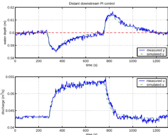
Figure 6 gives the experimental results obtained with the dis-tant downstream PI controller. A downstream withdrawal of 10 l/s (0.01 m3/s) is done at time t = 280 s. The controller is able to reject this unknown perturbation in about 400 s (time for the output y to meet the target yc = 0.6 m). The outlet is closed at

time t = 750 s, and the response appears to be symmetrical.

4.3 Local upstream control

Local upstream control is not subject to control performance limitations, since there is no delay between the actuator and the controlled variable (in fact, it can be shown that the trans-fer function is outer). However, the actuator dynamics induce physical limitation on the control.

The PI controller is tuned in order to have a gain margin of 12 dB (in order not to control the first resonant mode of the system) and at least 60 degrees of phase margin, see figure 7. The local upstream controller is given by:

K2(s) =

2s + 0.1

s

Figure 8 gives the experimental results obtained with the local upstream PI controller. The simulation with a linear model is

0 200 400 600 800 1000 1200 0.58 0.59 0.6 0.61 0.62 time (s) water depth (m)

Distant downstream PI control

measured y simulated y 0 200 400 600 800 1000 1200 0.04 0.045 0.05 0.055 time (s) discharge (m 3/s) measured u simulated u

Figure 6: Experimental response of the distant downstream PI controller to a downstream withdrawal, comparison with a lin-ear simulation Bode Diagram Frequency (rad/sec) Phase (deg) Magnitude (dB) −20 −10 0 10 20 30 40 50

60 Gm = 12.748 dB (at 0.88037 rad/sec), Pm = 115.52 deg (at 0.062733 rad/sec)

10−4 10−3 10−2 10−1 100 −225 −180 −135 −90 −45

Figure 7: Bode plot of K2G2for the local upstream controller

able to rather accurately reproduce the dynamic behavior of the system in response to a downstream withdrawal.

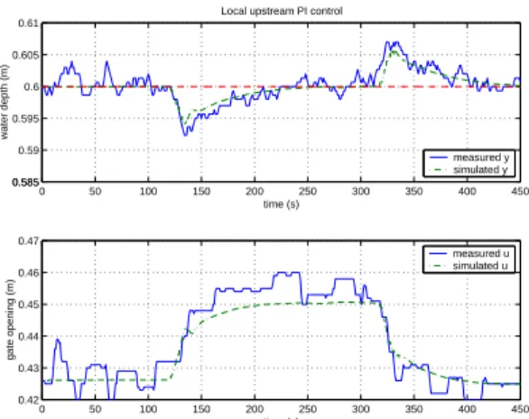
A downstream withdrawal of 10 l/s (0.01 m3/s) is done at time t = 120 s. The controller is able to reject this unknown pertur-bation in about 100 s, which is about 4 times quicker than with the downstream controller.

In the local upstream control case, the bandwidth is signifi-cantly higher than in the distant downstream control case. The measurement noise is then amplified by the control system. This explains the difference between the linear simulated con-trol and the measured one in figure 8 (there is a dead band of 5 mm on the control action u2). The measurement noise should be filtered in order to have a better fit. In fact, part of the gain margin is used to take this into account.

0 50 100 150 200 250 300 350 400 450 0.585 0.585 0.59 0.595 0.6 0.605 0.61 time (s) water depth (m)

Local upstream PI control

measured y simulated y 0 50 100 150 200 250 300 350 400 450 0.42 0.43 0.44 0.45 0.46 0.47 time (s) gate opening (m) measured u simulated u

Figure 8: Experimental response of the local upstream PI con-troller to a downstream withdrawal, comparison with a linear simulation

5

Conclusion

The paper has exposed and validated a methodology to design efficient automatic controllers for irrigation canals, based on the Saint-Venant model. The methodology has been applied on an experimental canal located in Portugal. The interest of the method is to greatly simplify the model calibration (a single experiment is needed to calibrate the model in steady state). Linear models around different reference points can then be obtained using recent results [9].

Two types of PI controllers were designed and field tested:

• a distant downstream PI controller, where the downstream water elevation y is controlled using the upstream dis-charge u1,

• a local upstream PI controller, where the downstream wa-ter level y is controlled using the downstream gate u2.

The experimental results are very satisfactory for classical PI controllers design for local upstream and distant downstream control. The proposed model-based methodology is therefore validated for PI controllers; these promising results will be gen-eralized to the control of multiple canal pools.

Acknowledgments

This work was supported by the French Embassy in Portugal and GRICES (Gabinete de Relac¸˜oes Internacionais da Ciˆencia e do Ensino Superior) of Portugal, through the scientific collab-oration project n◦547-B4 : “Mod´elisation hydraulique et tests de r´egulateurs automatiques pour le canal r´eduit d’ ´Evora”. The first two authors acknowledge the financial help of Cemagref and INRA through the collaborative program ASS AQUAE n◦02 on the control of delayed hydraulic systems.

References

[1] O.S. Balogun. Design of real-time feedback control for canal

systems using linear quadratic regulator theory. Ph.D. thesis,

Department of Mechanical Engineering, University of California at Davis, 1985. 230 pp.

[2] J.P. Baume and J. Sau. Study of irrigation canal dynamics for control purposes. In Int. Workshop RIC’97, pages 3–12, Mar-rakech, Morroco, 1997.

[3] G. Corriga, F. Patta, S. Sanna, and G. Usai. A mathematical model for open-channel networks. Applied Mathematical

Mod-elling, 3:51–54, 1979.

[4] J.A. Cunge, F.M. Holly, and A. Verwey. Practical aspects of

computational river hydraulics. Pitman Advanced Publishing

Program, 1980.

[5] A. Garcia. Control and regulation of open channel flow. M.Sc. thesis, University of California, Davis, 1988.

[6] H. Jreij. Sur la r´egulation des cours d’eau am´enag´es. Ph.D. thesis, Universit´e Paris-XI Dauphine, 1997. (in French). [7] P. Kosuth. Techniques de r´egulation automatique des syst`emes

complexes : application aux syst`emes hydrauliques `a surface libre. Ph.D. thesis, Institut National Polytechnique de Toulouse,

1994. (in French).

[8] A. Lencastre. Hydraulique g´en´erale. Eyrolles, SAFEGE, 1996. [9] X. Litrico and V. Fromion. Infinite dimensional modelling of open-channel hydraulic systems for control purposes. In 41st

Conf. on Decision and Control, pages 1681–1686, Las Vegas,

2002.

[10] X. Litrico and V. Fromion. Real-time management of multi-reservoir hydraulic systems using H∞ optimization. In IFAC World Congress, Barcelona, 2002.

[11] X. Litrico and V. Fromion. Advanced control politics and op-timal performance for an irrigation canal. In European Control

Conference, Cambridge, UK, 2003.

[12] X. Litrico, V. Fromion, and G. Scorletti. Improved performance for open-channel hydraulic systems using intermediate measure-ments. In IFAC Workshop on Time-Delay Systems, pages 113– 118, Santa Fe, 2001.

[13] P.-O. Malaterre. Mod´elisation, analyse et commande optimale

LQR d’un canal d’irrigation. Ph.D. thesis, ISBN

2-85362-368-8, Etude EEE n◦. 14, LAAS - CNRS - ENGREF - Cemagref, 1994. (in French).

[14] P.-O. Malaterre and J.-P. Baume. Sic 3.0, a simulation model for canal automation design. In Int. Workshop on the Regulation

of Irrigation Canals RIC’97, Marrakech (Morocco), April 22-24

1997.

[15] P.-O. Malaterre, D. C. Rogers, and J. Schuurmans. Classifica-tion of canal control algorithms. J. of IrrigaClassifica-tion and Drainage

Engineering, 124(1):3–10, January/February 1998. ISSN

0733-9437.

[16] J. Schuurmans. Control of water levels in open-channels. Ph.D. thesis, ISBN 90-9010995-1, Delft University of Technology, 1997.

[17] E. Weyer. System identification of an open water channel.