This work was supported in part by INESC-TEC Porto/Portugal, and in part by CNPq/Brazil and CAPES/Brazil.
Distribution System Reconfiguration with Variable
Demands Using the Opt-aiNet Algorithm
Simone S. F. Souza, Ruben Romero
, Senior Member IEEE Electrical Engineering DepartmentUNESP – Univ. Estadual Paulista Ilha Solteira, SP, Brazil
simonefrutuoso.mat@gmail.com, ruben@dee.feis.unesp.br
Jorge Pereira
INESC TEC and Faculty of Economics, University of PortoPorto, Portugal
jpereira@inesctec.pt
João T. Saraiva
INESC TEC and Faculty of Engineering, University of PortoPorto, Portugal
jsaraiva@fe.up.pt Abstract—This paper describes the application of the Opt-aiNet
algorithm to the reconfiguration problem of distribution systems considering variable demand levels. The Opt-aiNet algorithm is an optimization technique inspired in the immunologic bio system and it aims at reproducing the main properties and functions of this system. The reconfiguration problem of distribution networks with variable demands is a complex problem that aims at identifying the most adequate radial topology of the network that complies with all technical constraints in every demand level while minimizing the cost of power losses along an extended operation period. This work includes results of the application of the Opt-aiNet algorithm to distribution systems with 33, 84, 136 and 417 buses. These results demonstrate the robustness and efficiency of the proposed approach.
Index Terms—Distribution System Reconfiguration, Variable Demands, Artificial Immune Systems, Opt-aiNet.
I. INTRODUCTION
Electrical companies are currently directing large investments to distribution systems in order to modernize them and to improve their automation level. These investments are designed to improve the reliability, the efficiency and the security of these systems. In this scope a lot of work has also been done at the scientific level namely to address the reconfiguration problem of distribution networks usually termed as DSR, Distribution System Reconfiguration.
The DSR problem is a complex and combinatorial problem that can be modeled as a mixed-integer nonlinear programming (MINLP) problem [1]. The DSR problem consists of identifying the best radial topology for an Electrical Distribution Systems (EDS) through the opening and closing of switches, so that it is optimized an objective function, which typically corresponds to the minimization of the active power losses. In this paper, the DSR problem is addressed considering variable demand levels, the objective function is the minimization of the cost of the energy losses along the planning period, always subject to the technical operation constraints of the EDS, such as the radiality condition, nodal voltage limits, branch current capacity limits, and satisfying the first and the second Kirchhoff Laws.
The DSR problem is difficult to solve using exact mathematical methods, as there are many combinations of solution candidates. Therefore, an alternative consists of using
intelligent optimization techniques, such as heuristic and meta-heuristics algorithms, artificial neural networks, artificial immune systems, among others. These techniques include effective strategies that enable reducing the search space and finding the best solution or at least good quality solutions.
In this sense, the literature related with the DSR problem assuming fixed demand levels includes publications reporting the use of heuristic algorithms [1-2], metaheuristics as Genetic Algorithms [3], Simulated Annealing [4], Tabu Search [5], Ant Colonies [6], GRASP [7], Artificial Neural Networks [8] and Artificial Immune Systems [9]. On the other hand, references [10-13] address the DSR problem assuming variable demand levels.
This paper describes the application of the Artificial Immune Network for Optimization (Opt-aiNet) to the DSR problem with variable demands [14]. In order to evaluate the quality of each candidate radial topology it is run a power flow study specially designed to address radial networks [15] for each demand level to be analyzed. As a result, it is possible to obtain the cost of energy losses along the specified operation period. In order to illustrate the application of the Opt-aiNet, this paper includes results obtained for distribution networks with 33, 84, 136 and 417 buses. These results confirm the robustness and the efficiency of the proposed approach.
II. OPT-AINET ALGORITMH
The Opt-aiNet algorithm was originally proposed in [14], and it represents an extension of the aiNet to solve optimization problems. It can be described as presented in the following steps.
Step I: Generate a population (P) with N antibodies;
Step II: Evaluate the affinity (objective function) for each antibody in the population P and store the mean of the population’s affinity in OldAffinity;
Step III: While the criterion of stabilization of the population is not satisfied repeat steps a. to g. as follows:
a. Generate Nc clones for each antibody of the
population (P) forming subsets of antibodies comprising the original antibodies (father antibody) and its clones; b. Submit the Nc clones of each father antibody to a
c. Evaluate the affinity (objective function) of each matured clone;
d. For each subgroup composed by a father antibody (original antibody) and its respective matured clones, select the antibody with the best affinity and remove the others, leaving the population P with the best antibodies of each subgroup through an elitist process;
e. Store the mean of the population’s affinity in NewAffinity;
f. Check the stabilization criterium: if the percentual difference between OldAffinity and NewAffinity is larger than a specified threshold percentage, OldAffinity*est then go to III.g. Otherwise, end this internal cycle and go to Step IV;
g. Update OldAffinity NewAffinity and return to a.; Step IV: Eliminate all antibodies of the population that have a resemblance larger than a threshold S (similarity rate) in the clonal suppression;
Step V: If the size of the population P is lower than N, generate as many antibodies as necessary to complete the population;
Step VI: If the stopping criterion is not satisfied, go back to the Step III, otherwise, stop.
The antibodies correspond to candidate solutions and each antibody generates a total number of Nc clones. According to
[16], the number Nc of clones generated in Step III.a for each
antibody i is given by (1). In this expression β is a multiplicative factor in [0,1], N is the total number of antibodies in the population P, and round(.) is the operator that outputs the nearest integer of its argument.
) ( i N round Ni c= β (1)
Following [16], the mutation rate α of each clone is given by (2). In this expression ρ is a parameter that controls the output of the exponential function and f* is the normalized value of the affinity function.
*) exp( ρf
α= − (2)
The f* parameter is calculated using (3) for minimization problems [16]. In these expressions, fmax represents the
maximum value of the affinity function.
max *
f f
f = (3)
The number of mutations affecting each clone of an antibody [17] is given by (4). In this expression m is the number of mutations that will affect a clone of an antibody, round(.) is the operator that outputs the nearest integer of its argument and N(0,1) is value taken from a Gaussian probability function with 0 mean and standard deviation 1.
)) 1 , 0 ( * ( N round m=
α
(4)III. PROPOSED METHODOLOGY
This section details the application of the Opt-aiNet algorithm described in Section II to the solution of the DSR problem with variable demand levels.
A. Coding of the Candidate Topologies
In this work we used the coding proposed in [18] for the DSR problem. In this coding scheme, the EDS is represented as a tree (graph theory) constituted by an array of arcs (branches). The encoding vector has dimension nl (number of
branches) and it represents the entire electrical system through all its branches. In this coding scheme the first (nb-1) elements
of the vector are the branches included in the radial topology (subset N1), and the branches between positions nb and nl
(subset N2), are the connection elements (branches off the radial configuration), as illustrated in Figure 1.
Figure 1. Codification vector for the 14-node system.
For example, Figure 2 displays a radial topology for this 14 nodes distribution network. This topology can be represented as (5), where all elements between 1 and (nb-1)
belong to the network topology. These elements are represented by continuous segments in the Figure and constitute a tree of the associated graph. The other elements, from nb til the end of the vector, are disconnected in this
configuration and are in dotted segments in Figure 2. This representation is not fixed, given that the same topology can be represented for instance as (6), which can help to diversify the search depending on the kind of operators that are used.
[C1C5C10C2C7C11C3C6C12 C4 C8 C13 C9 (C14C15C16)] (5)
[C1C2C3C4C5C6C7C8C9C10 C11 C12 C13 (C14C15C16)] (6)
Figure 2. Example of codification to the 14-node system.
This codification ensures that the initial population only includes radial topologies. Therefore, it is possible to develop search operators that preserve the radiality of the topology, thus avoiding this type of infeasibility.
B. Strategy to Generate the Initial Population
To generate the initial population (P) including N elements for the Opt-aiNet algorithm, we used the Prim heuristic detailed in [18]. This heuristic uses the codification detailed in the previous section and it is described in the next steps. From each run it yields a radial topology and so it is applied as many times as the number of elements in the population.
Step I: D is the set of nodes included in the current configuration;
Step II: Set
D
=
φ
, N1=φ
, N2=φ;Step III: Add to D the node associated to the system substation. This node is taken as the root node;
Step IV: Find all branches with a vertex in D;
Step V: Randomly select a branch identified in the previous step to enter in the current topology;
Step VI: If the selected branch generates a loop in the topology, include it in N2, otherwise include the opposite vertex of that branch in D and the branch in N1;
Step VII: Go back to Step III until all branches are selected. At the end of the process, the vector [N1, N2] represents a radial topology of the EDS. This strategy always generates topologically feasible solutions from the radial point of view, contributing to the efficiency and diversity of the algorithm proposed in this paper.
C. Operator to Evaluate the Affinity
The operator to evaluate the affinity is used to characterize the quality of each candidate solution (each antibody) in the population P. This value is related with the cost of the energy losses associated with that topology when supplying a specified demand level in each bus. In order to obtain the losses it is run a power flow study specially designed to address radial networks [15]. It is important to mention that if a particular topology associated with an antibody is infeasible from a technical point of view (namely because nodal voltage limits or branch current limits are violated) it is penalized after running the power flow and getting the value of the losses. If several demand scenarios are under analysis, then a power flow exercise is run for each of them and at the end (7) is used to obtain the affinity value of the associated topology. In this expression Nd is the number of demand levels to be analysed,
Ti and Pi are the duration and the power losses associated with
the demand level i and Ki is the cost of energy for period i.
] P * T * K [ f Nd i i 1 i i = = (7) D. Cloning Operator
In the cloning process, it is generated a subpopulation of clones (C). The subpopulation consists of Nc clones obtained
from the antibodies of the subpopulation P{n}. The number of
clones generated by each antibody is calculated using (1).
E. Hypermutation Operator
In the hypermutation process, it is necessary to calculate in the first place the number of mutations of an antibody i in the iterative process of the Opt-aiNet using (4). Equation (2) defines the mutation rate (α), and (3) establishes the normalized affinity (f*). Following these calculations, a random mutation is performed as described in the next steps. Step I: Read C and obtain Nc (number of clones);
Step II: For each clone in the population C, calculate the number of mutations (m) and do:
a. Select randomly a circuit l ∈ N2 to each antibody. This position l represents a disconnected circuit;
b. Connect/close the selected circuit and identify the loop that is formed. Choose a circuit in the loop that was formed and replace it by the circuit l;
Step III: Store in C* the matured antibodies and return C*; Figure 3 presents an illustrative example of the hypermutation process. In this example it was used the antibody modeled by (6). In this process, it was initially randomly chosen a branch belonging to set N2, i. e., a disconnected circuit. After this process, this circuit is connected and a loop is formed in the system. This loop should be identified and stored. Then, it is randomly chosen another branch belonging to the mentioned loop to replace the initial branch. Finally the branches are exchanged (branch 15 is replaced by branch 11in this example), generating a matured antibody. This hypermutation strategy always generates topologically feasible antibodies.
Figure 3. Illustration of the hypermutation process. F. Selection Operator
During the iterative process of the Opt-aiNet algorithm an elitist selection process is carried out, so that the antibody with the best affinity within each subset of antibodies (father antibody and its matured clones) always remains in the population P after the processes of cloning and hypermutation. This process ensures that in each iteration of the algorithm the best antibodies are never replaced by worse affinity antibodies.
G. Stoping Criterion for the Internal Iterative Process
The internal iterative process finishes when the population is stabilized, that is, when the variation between the average values of the population’s affinity for two consecutive iterations during this process is smaller than a threshold. If the average value of the population’s affinity does not change from one iteration to the next more than a pre-established percentage, then the population is considered to be stable and the hypermutation process ends.
H. Clonal Supression Process
In the clonal suppression process, the population P is evaluated by comparing the similarity between its antibodies. If the similarity between a pair of antibodies is larger than a threshold S (similarity rate), then one of the antibodies is discarded through the clonal suppression process. In this comparison an index of similarity between the topologies is calculated and used to make the decision. As a result, similar
antibodies are eliminated in order to provide greater population diversity.
I. Control of the Population’s Size
After the clonal suppression process, the algorithm checks if the population size is lower than N. If so, new antibodies are randomly generated using the heuristic presented in subsection III.B in order to complete the population.
J. Stoping Criteria
The Opt-aiNet algorithm stops if the affinity value of the best antibody in the population did not change for a specified number of iterations and the average of the affinity value of all the antibodies in the population doesn’t change more than a specified percentage along a specified number of iterations. If the two above conditions hold simultaneously, then the algorithm ends indicating that a final solution was obtained. If not, the iteration counter is increased by 1. If the maximum number of iterations was reached then the algorithm stops indicating that a final solution was not obtained. If not, it returns to Step II to start a new iteration.
IV. APPLICATIONS AND RESULTS
This section presents the results that were obtained using the Opt-aiNet algorithm to solve the DSR problem with variable demand levels. The Opt-aiNet algorithm was implemented in the Borland C++ 6.0® [19] platform. In order to obtain the power active losses for each demand level and for each candidate solution (each antibody in the population) we used the power flow algorithm detailed in [15]. The tests were developed using distribution systems with 33, 84, 136 and 417 buses and the respective data is available in [20], [21], [5] and [22]. The systems with 33, 84 and 136 nodes are test systems and the one with 417 nodes is a real distribution network. Their nominal voltages are 12.66 kV, 11.40 kV, 13.80 kV, and 11.00 kV, respectively.
A. Demand Scenarios
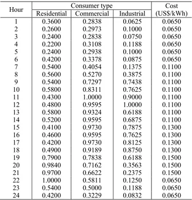
The tests were developed using a period of 24 hours and for each of them it was specified a demand level for each node in the system. The demand was organized in three classes as follows (a) residential, (b) commercial and (c) industrial and for each of them a typical load diagram was specified, such as presented in Table I using load factors. In order to define the demand levels in the system along the 24 hours, it was randomly selected the type of demand connected to each bus assuming that 60% of the buses have residential consumers, 25% have commercial and 15% industrial and also admitting that in each bus there is just one type of consumer [12]. Then, for a specific bus and for a given hour, the active and reactive peak powers in that bus are multiplied by the load factor of that hour for the type of consumer (residential, industrial and commercial) that was initially sampled for that bus.
Table I also presents the cost of energy in each hour, i. e., along the 24 hours of the simulation period. In each hourly period, these values are multiplied by the active power losses calculated by the power flow study in order to obtain the value of the affinity function associated with a particular antibody that is with a candidate topology solution.
TABLE I. Load factors of the consumers and cost of energy losses.
Hour Residential Consumer type Commercial Industrial (US$/kWh) Cost
1 0.3600 0.2838 0.0625 0.0650 2 0.2600 0.2973 0.1000 0.0650 3 0.2400 0.2838 0.0750 0.0650 4 0.2200 0.3108 0.1188 0.0650 5 0.2400 0.2938 0.1000 0.0650 6 0.4200 0.3378 0.0875 0.0650 7 0.5400 0.4054 0.1375 0.1100 8 0.5600 0.5270 0.3875 0.1100 9 0.5400 0.7297 0.7438 0.1100 10 0.5800 0.8311 0.7625 0.1100 11 0.4300 1.0000 0.9000 0.1100 12 0.4800 0.9595 1.0000 0.1100 13 0.5800 0.9324 0.6188 0.1100 14 0.5200 0.9595 0.6875 0.1100 15 0.4100 0.9730 0.7875 0.1300 16 0.4600 0.9595 0.7625 0.1300 17 0.4200 0.9730 0.8125 0.1300 18 0.4900 0.9189 0.8750 0.1300 19 0.7900 0.7838 0.6188 0.1500 20 0.9840 0.7162 0.3563 0.1500 21 0.9700 0.6622 0.2375 0.1500 22 1.0000 0.5811 0.1250 0.0650 23 0.5400 0.5000 0.1188 0.0650 24 0.4200 0.3229 0.0832 0.0650
B. Parameters of the Opt-aiNet Algorithm
The tests using the four mentioned distribution systems were conducted using the parameters in Table II where ε is the tolerance used in the power flow algorithm detailed in [15]. These parameters were established after running the Opt-aiNet algorithm in a number of trial tests.
TABLE II. Parameters used in the Opt-aiNet.
Paramters 33-, 84-, 136- Distribution system 417-
N 40 60 β 0.3 0.3 Ger 50 90 Ρ 4 5 S 80% 80% est 1% 1% Ε 10-6 10-6
C. Systems with 33, 84, 136 and 417 nodes
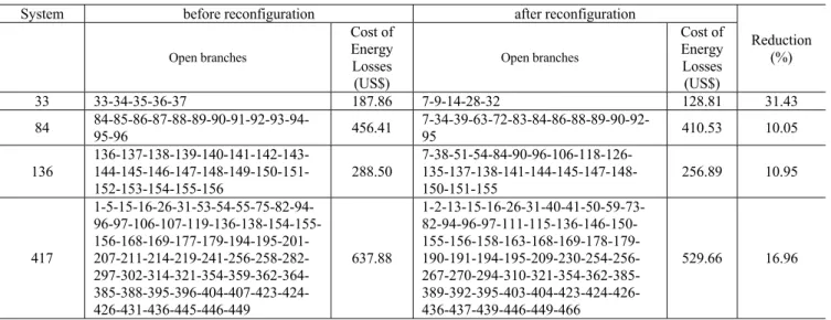
For each tested system, Table 3 presents the disconnected branches in the initial topology and in the final topology that was identified using the Opt-aiNet algorithm, that is after reconfiguration. This table also indicates the cost of energy losses for both topologies as well as the reduction that was obtained. The use of the Opt-aiNet led to a reduction from 10% to 31% in the cost of energy losses when going from the initial to the final topology.
For the 33-, 84-, 136- and 417-node systems, the Opt-aiNet algorithm found the best solutions reported in the literature, such as presented in [12-13]. Finally, the average time to obtain the results was 0.258, 4.095, 25.723 and 174.232 seconds, respectively.
TABLE III. Results for the 33-, 84-, 136-, and 417-node systems.
System before reconfiguration after reconfiguration
Reduction (%) Open branches Cost of Energy Losses (US$) Open branches Cost of Energy Losses (US$) 33 33-34-35-36-37 187.86 7-9-14-28-32 128.81 31.43 84 84-85-86-87-88-89-90-91-92-93-94-95-96 456.41 7-34-39-63-72-83-84-86-88-89-90-92-95 410.53 10.05 136 136-137-138-139-140-141-142-143- 144-145-146-147-148-149-150-151-152-153-154-155-156 288.50 7-38-51-54-84-90-96-106-118-126- 135-137-138-141-144-145-147-148-150-151-155 256.89 10.95 417 1-5-15-16-26-31-53-54-55-75-82-94- 96-97-106-107-119-136-138-154-155- 156-168-169-177-179-194-195-201- 207-211-214-219-241-256-258-282- 297-302-314-321-354-359-362-364- 385-388-395-396-404-407-423-424-426-431-436-445-446-449 637.88 1-2-13-15-16-26-31-40-41-50-59-73- 82-94-96-97-111-115-136-146-150- 155-156-158-163-168-169-178-179- 190-191-194-195-209-230-254-256- 267-270-294-310-321-354-362-385- 389-392-395-403-404-423-424-426-436-437-439-446-449-466 529.66 16.96 V. CONCLUSION
This paper describes the application of the Opt-aiNet algorithm to the Distribution System Reconfiguration problem considering variable demands that change along the planning period, 24 hours in this case. The search for the most adequate topology is driven by the minimization of the cost of energy losses, assuming that the energy cost also varies along the day. The Opt-aiNet algorithm was tested using 4 distribution systems, with 33, 84, 136 and 417 buses and in all analyzed cases the Opt-aiNet was able to identify topologies that are feasible from a technical point of view and also better regarding solutions provided in the literature. Finally, the Opt-aiNet algorithm had a very satisfactory behavior, namely considering its robustness and efficiency.
REFERENCES
[1] A. Merlin, H. Back, “Search for a minimal-loss operating spinning tree configuration in an urban power distribution system,” in Proc. 1975 Power System Computation Conference, pp. 1-18.
[2] S. Civanlar, J. J. Grainger, S. S. H. Lee, “Distribution feeder reconfiguration for loss reduction”, IEEE Transactions on Power Delivery, vol. 3, n. 3, pp. 1217-1223, 1988.
[3] K. Nara, A. Shiose, M. Kitagawa, T. Ishihara, “Implementation of genetic algorithm for distribution systems loss minimum reconfiguration”, IEEE Transactions on Power Systems, vol. 7, n. 3, pp. 1044-1051, 1992.
[4] H. C. Chang, C. C. Kuo, “Network reconfiguration in distribution systems using simulated annealing”, Electric Power Systems Research, vol. 29, n. 3, pp. 227-238, 1994.
[5] D. Zhang, Z. Fu, L. Zhang, “An improved TS algorithm for loss-minimum reconfiguration in large-scale distribution systems,” Electric Power Systems Research, vol. 77, n. 5-6, pp. 685-694, 2007.
[6] E. Carpaneto, G. Chicco, “Distribution system minimum loss reconfiguration in the hyper-cube ant colony optimization framework”, Electric Power Systems Research, vol. 78, pp. 2037-2045, 2008. [7] S. S. F. Souza, M. Lavorato, R. Romero, “Specialized GRASP applied
to the problema of distribution reconfiguration systems”, In Proc. IEEE PES Transmission and Distribution Latin America (T&D-LA), 2012, pp. 1-6. (in Portuguese).
[8] H. Salazar, R. Gallego, R. Romero, “Artificial neural networks and clustering techniques applied in the reconfiguration of distribution systems,” IEEE Transactions on Power Delivery, vol. 21, n. 3, pp. 1735-1742, 2006.
[9] S. S. F. Souza, R. Romero, J. F. Franco, “Artificial immune networks Copt-aiNet and Opt-aiNet applied to the reconfiguration problem of
radial electrical distribution systems,” Electric Power Systems Research, vol. 119, pp. 304-312, 2015.
[10] E. A. Bueno, C. Lyra, C. Cavellucci, “Distribution network reconfiguration for loss reduction with variable demands,” in Proc. 2004 IEEE Latin America Transmission and Distribution Conference, pp. 384-389.
[11] L. M. O. Queiroz, C. Lyra, “Adaptive hybrid genetic algorithm for techinical loss reduction in distribution networks under variable demands,” IEEE Transactions on Power Systems, vol. 24, n. 1, pp. 445-453, 2009.
[12] L. H. F. M. Possagnolo, Distribution systems reconfiguration operating in several demand levels through of the variable neighborhood search (Marter Thesis), Campus of Ilha Solteira, Unesp, Univ Estadual Paulista, 2015. (In Portuguese)
[13] S. S. F. Souza, R. Romero, J. Pereira, J. T. Saraiva, “Distribution System Reconfiguration with variable demands using the Clonal selection Algorithm”, In Proc International Conference on Intelligent System Application to Power Systems (ISAP), 2015, pp. 1-6.
[14] L. N. de Castro, J. Timmis, “An artificial immune network for multimodal function optimization”, In Proc. of IEEE World Congress on Evolutionary Computation, 2002, pp. 699-704.
[15] D. Shirmohammadi, H. W. Hong, A. Semlyen, G. X. Luo, “A compensation based power flow method for weakly meshed distribution and transmission networks”, IEEE Transactions on Power Systems, vol. 3, n. 2, pp. 753-762, 1988.
[16] L. N. de Castro, “Immune engineering : development and application of computational tools inspired by artificial immune systems”, 2001, PhD. Thesis, UNICAMP, Campinas/Brazil. (in Portuguese).
[17] F. O. de Franca, F. J. Von Zuben, L. N. de Castro, “An Artificial Immune Network for Multimodal Function Optimization on Dynamic Environments”, In: Proc. GECCO, 2005, pp. 289–296.
[18] E. M. Carreño, R. Romero, A. P. Feltrin, An efficient codification to solve distribution network reconfiguration for loss reduction problem. IEEE Transactions on Power Systems, vol. 23, n. 4, pp. 1542-1551, 2008.
[19] Borland 6.0 Version, C++ Builder.
[20] M. E. Baran, F. F. Wu, “Network reconfiguration in distribution systems for loss reduction and load balancing,” IEEE Transactions on Power Delivery, New York, vol. 4, n. 2, pp. 1401-1407, 1989. [21] J. P. Chiou, C. F. Chang, C. T. Su, “Variable scaling hybrid differential
evolution for solving network reconfiguration of distribution systems”, IEEE Trans. on Power Systems, vol. 20, no. 2, pp. 668-674, 2005. [22] J. L. Bernal-Agustin, Application of genetic algorithms to the optimal
design of power distribution systems. 1998. 346 f. Tesis, University of Zaragoza, Zaragoza, 1998.