Primary public health care and socioeconomic asymmetries in Portugal

(1)

Primary Public Health Care and

Socioeconomic asymmetries in Portugal

Rafael Ribeiro Barbosa

Student number – 419

A project carried out with the supervision of Professor Pedro Pita Barros

(2)

Abstract

In this work project, we set out to study the determinants of regional discrepancies in terms of demand for different Primary public health care providers in Portugal for the year of 2009, more specifically if regions with higher purchasing power present greater slices of public health expenditures devoted to hospitals. Results point to a confirmation of this theory. Reasons for this possible behavior include differences in perceived health care needs and higher tolerance for bureaucracy associated with hospitals. Data used was provided by the administration of the Portuguese NHS (ACSS). We use a model for fractional response variables to study the problem.

Keywords:

Primary health care Hospital

Fractional response variables Socioeconomic asymmetries

(3)

1. Introduction

The constant growth of Health expenditures has become an undeniable reality in all developed countries throughout the world, a trend that has not always been accompanied by an equivalent movement in wealth, causing the share of wealth devoted to this area to rise in a persistent fashion1_{. As it is known, in most developed countries,} a great part of this spending is actually supported by the State. This reality has forced Governments to accept the pressing need to contain the growth of health care expenditures as a way to guarantee the sustainability of this side of the social welfare state which is one of the cornerstones of today’s western societies. However, cutting the number of services rendered or increasing the share of the price to be paid by the citizens has always been regarded as a last resort measure and a step back in terms of acquired rights. To avoid this possibility, it is therefore understandable that arriving at an efficient use of resources becomes the prime objective, as it is a way to decrease expenditures without compromising the continued provision of the same level of health care goods and services.

For Portugal, a country where the National Health System (NHS) was ideally envisioned to be universal and mostly free of charge at the moment of use and with well known problems regarding economic growth and public finances, this could not be truer. As such, the necessity to maximize efficiency of resource allocation to reduce costs and meet the preferences of the population has become apparent to recent governments.

One of the areas in which the preoccupation about misallocation of resources exists is primary care. The definition of this concept usually revolves around the medical care a patient first receives upon contact with the health care system, sometimes

(4)

followed by referral to other health care providers. The exact definition found in

Defining Primary Care: An Interim Report (IOM, 1994b) is “the provision of integrated, accessible health care services by clinicians who are accountable for

addressing a large majority of personal health care needs, developing a sustained

partnership with patients, and practicing in the context of family and community.” It is

clear that a proper organization of this “door” to the NHS is crucial to a good functioning of the system as a whole.

In Portugal, public primary care can be obtained in two ways: either by going to a primary care center (PCC) or by directly resorting to a Hospital, a choice which is in great part made solely by the user. This situation makes clear that the allocation of human and technical assets between these two should try to reflect the preferences of the population that it is meant to service. Failure to achieve this, can lead to having either idle or insufficient resources in a determined primary care facility and an excess in others, a luxury that the increasingly restrained budget of the Portuguese NHS does not allow. For this reason the Administration of the Portuguese NHS (ACSS) has shown interest in studying this phenomenon.

Statistical evidence seems to point that the preferences of the population regarding this choice are indeed heterogeneous and that some factors tend to strongly influence this choice. According to ACSS, income is seen as one of these factors, for reasons supposedly related with different perception of gravity of medical conditions and different ability to deal with bureaucratic entanglements of hospitals.

The relationship between income and demand for health care is not new. In 1971 Julian Hart coined the term Inverse Care Law1_{, which stated that the availability of} good medical or social care tends to vary inversely with the need of the population

(5)

served, that is, the supply of medical care tends to be more concentrated in richer regions where the overall health of the population is, on average, better. This theory has been widely debated throughout the years, but there is a strong support for it, as well as studies that demonstrate it empirically. One study looked at the effect of socioeconomic deprivation on waiting times for cardiac surgery. Deprived patients were more likely to develop coronary heart disease but less likely to be investigated and undergo surgery1_. The hypothesis that socioeconomic factors, besides the quantity of health care, can also influence the choice between the providers of primary care (Hospital vs. PCC in this case) is, therefore, just an extension of this theory. An extension that can affect real policy making decision by, for example, giving a sense of which type of infrastructures might need to be invested in, or whether existing resources should be reallocated, in order to have the sufficient capacity to meet future regional demand. Existing literature regarding this specific type of potential impact, in Portugal or otherwise, was not found.

This work project attempts to test this hypothesis. For that we use data of Hospital and PCC expenditure in Portugal and check whether the percentage of relative Hospital expenditures in Portugal tends to be higher in areas with higher purchasing power, after accounting for differences in other demographic variables and in the structure of the supply of health care.

In the second part of this paper we will describe the raw data we worked with and how it was transformed in order to obtain the final database that was used.

In the third part we will first discuss the methodology used, namely in terms of econometric analysis, because we decided to use a fractional response variable as the dependent variable for the main model. For this reason we start with a literature review on this issue and then move to actually present our model.

1 _{Pell JP, Pell AC, Norrie J, et al, BMJ. 2000, “Effect of socioeconomic deprivation on waiting time for}

(6)

Afterwards, we present and analyze the econometric results of our model and discuss its implications. Generally, these results point to a confirmation of the perception that a relation with socioeconomic factors exists while uncovering other important determinants, such as percentage of population with family doctors. We also discuss hypothetical future scenarios in which the dependent variable is influenced by changes in the explanatory variables.

Finally, we move to the conclusion where we will summarize our findings.

2. Data (Sources and construction of database) 2.1 Sources

The information used in this work project can be divided into two categories: the medical information and the socio-demographic information. The latter was, for the most part, acquired in the website of the Portuguese national statistics institute (INE). The first is information concerning the activities of Portuguese hospitals and primary care centers which was provided by ACSS (Administração Central do Sistema de Saúde), the central administration of the Portuguese NHS. The hospital related data and the primary care center data were provided in two separate and different datasets, the GDH and ACES, respectively. The nature of both of these databases will be explained in more detailed next.

2.1.1 GDH

The GDH (Grupos de Diagnóstico Homogéneo), similar to the English Diagnosis Related Groups, is a hospital patient classification system that groups patients in clinically coherent groups from the point of view of resource consumption. It allows the definition of the output of the hospital, which is ultimately translated in the amount of

(7)

goods and services that each patient receives in accordance with the needs of his pathology. The adoption of this framework in the Portuguese NHS goes back to the beginning of the 1990’s, although the current version of this system was approved in June of 20061_{, using a grouping system similar to the one used in the United States.} Each diagnosis group has a relative weight associated with it, meant to reflect the expected treatment cost in which the NHS will have to incur.

The database provided by ACSS consists of a detailed record of all hospital admissions in Portugal from 2006 through 2010 containing a wide range of information on each observation, from the age, gender, date of admission, date of exit, etc. However, the most relevant data for the analysis is the residence of the patient, the cost incurred by the NHS for each episode of a determined GDH and, obviously, the GDH code associated with each observation.

2.1.2 ACES

The ACES (Agrupamentos Centros de Saúde) are an administrative geographical division of all primary care centers in Portugal under different regional headquarters that coordinate and manage the centers within its jurisdiction, with the purpose of enabling a more efficient management of primary care centers throughout the country. The law approving the creation of this new framework was passed in March of 20092_. There are a total of 74 ACES in Portugal, with most of them being a grouping of counties (“concelhos”) even though some of them, in the most populated counties of Lisbon and Oporto, have to be divided in terms of parishes (“freguesias”). Additionally, some ACES were also grouped into ULC’s (Unidade Local de Saúde), like the cases of the ULC of Castelo Branco which incorporates the ACES of Beira

1_{Portaria nº 567/2006 of June 12}th

(8)

Interior Sul and Pinhal Interior Sul, and the ULC of Norte Alentejo that consists of the ACES of Caia and São Mamede.

Unlike with the GDH, the database provided by ACSS with information on primary care centers consists of aggregate information on each ACES, in terms of medical and socio-demographical population characterization, resources allocation, overall cost structure as well as other miscellaneous information. The information on the ACES spans the years from 2006 until 2009.

2.2 Building the database

The purpose which we set out to accomplish with this work project obviously implies an association between the hospital and primary care center data, however, the fact that one existed only at an aggregate level while the other was much more detailed, made a direct relationship impossible. Instead, the information contained in the GDH database had to be aggregated to somehow match the geographical identification of the primary care center grouping. The consequence of this fact is that the ensuing analysis has to be done in a macro level in which we compare across regions. This approach naturally has a tendency to hide important information when compared to a scenario in which we have much more detailed and discriminated choices by individual decision makers (a description of the ideal data and respective treatment required for this type of analysis is presented in the beginning of the Methodology section). The final choice was to perform the analysis at a county level (excluding the autonomous regions of Madeira and Açores) leaving us with a total of 281 observation. In regards to the time horizon, we choose to conduct the analysis looking only at the year of 2009, which is the most recent year for which there is information for both the GDH and the ACES databases.

(9)

Combining all this information in a single coherent database was the first challenge of the analysis and it involved several steps. First, due to the choice of geographical scope, research had to be performed regarding the distribution of counties and parishes among ACES and a matching process was made1_{. This allowed us to} assign to each county the relevant statistical information of the respective ACES.

A second problem was that the exact distribution of primary care center costs among counties was unknown (only existed at an ACES level), so it was decided to divide it amongst the counties, using as weight the percentage of the county population in the total ACES population in hopes this would be a good estimate. It should be noted that the figure for the ACES population concerns the year of 2009, while the county population, retrieved from INE, concerns 2011, but assuming that the variations were not that significant (which is reasonable because Portuguese population presents very low growth rates), this should not affect the overall results.

Thirdly, we aggregated the GDH occurrences by county of residence of the patient. As previously mentioned, each diagnosis in the GDH has a weight associated with it, but it also has a price, designed to reflect an approximate cost incurred by the NHS in treating the patient. This price was not initially contained in the GDH database so it had to be incorporated. To do this, we generated a variable identical to the GDH code called price. We then replaced all the observations with a determined GDH by the respective price2 _{(Appendix 3). Subsequently, we summed all the occurrences of the} variable price by county3_{. All other information was discarded in the process. In the end} we were left with the variable county and the total hospital spending for the each county in the year of 2009. This information was then used to build the dependent variable in our model as will be explained in the methodology section.

1 _{This was done using the Portuguese legislation regarding ACES (already mentioned in section 2.1.2.)} 2 _{Using the command “replace” in Stata}

(10)

Finally, we used the INE databases to determine and include in the database relevant population characteristics that were likely to influence the dependent variable. These include percentage of female population, population density, percentage of population with tertiary education, indexes for elder and youth population and number of doctors per 1000 inhabitants. Only after this process could we start our analysis.

3. Methodology

Before we introduce the methodology for the model used in this project, it is important to discuss what would be the most desirable data that we could have in order to perform the most precise and reliable analysis of the problem possible. This is useful to ensure a deeper understanding of the problem at hand, serve as comparison with the model that was ultimately chosen and see how the lack of ideal information was overcome and how it conditioned the analysis.

First of all, it is important to realize that, since we are trying to explain whether socioeconomic factors have an influence in the choice between going to a Primary Care Center or a Hospital emergency room, the optimal dependent variable in the analysis would be a binary variable which would, for example, assume the value 0 if the patient decided to go to a primary care center and 1 if the patient decided to go to the hospital. This ideal database would obviously only include cases in which such a choice is plausible. We would not, for instance, include observations relating to visits to the Hospital’s emergency room because of severe burns in a significant part of his body, as this is clearly a medical emergency which Primary Care Centers are not best suited to deal with. We would then use as explanatory variables the relevant characteristics of each particular individual associated with each observation, such as his income, education, age, gender, distance from his home to the nearest hospital and to the nearest

(11)

primary care center, relevant medical conditions, etc. Since we would be dealing with a binary variable, we would use a Probit or Logit model, instead of simple OLS regression. If, by the end, we discovered that the coefficients associated with the relevant socioeconomic variables were statistically significant we would have reliably proven that individuals with different levels of income have different preferences regarding their choice for public primary health care.

This of course would imply tremendous amounts of information which is not available. To begin with, we don’t have any socioeconomic data of the user associated with each observation in neither database. This problem could be easily circumvented by using the socioeconomic information of his county of residence, despite the fact that this would imply that we would be completely ignoring asymmetries within each county. Regardless, that is not the most worrying problem. As we have seen when we described the data in the previous section, the kind of detailed information about Primary care center episodes required to even start using this approach does not exist. Instead, we only have information on aggregate total costs for each ACES rather than data on individual episodes of Primary care centers throughout the country. This renders the hypothesis of going through with the “ideal” binary model addressed above, utterly unfeasible. As such, another approach had to be devised.

The model that we have built uses as dependent variable the percentage of hospital expenditure in total health expenditure for a region (county in this case), given by the sum of hospital expenditure plus total primary care center costs. Here, hospital expenditure, as mentioned before, is obtained through the summation of all hospital diagnosis multiplied by the price associated with the respective diagnosis. Given that the NHS price of each diagnosis is the same for all regions of the country, the regional discrepancies must therefore be explained either by a volume effect (one county

(12)

presenting more diagnoses), by a composition effect (one county with a higher incidence of diagnoses that are more costly to the NHS), or by a combination of the two. We expect that, if it is true that income influences the choice of primary care provider, we are going to find that, ceteris paribus, in counties with higher purchasing power the quantity of hospital episodes should increase and the number of primary care center episodes decrease. Naturally, this would positively impact our dependent variable on an aggregate level.

Before we move on, it is important to characterize this variable so we know what type of variation we are trying to explain. The mean of this measure of relative hospital expenditure is 77.12% and presents a standard deviation of 4.32%. The county with the lowest figure at a national level was Vizela in ACES of “Ave II – Guimarães/ Vizela” with only 63.8% of total public health expenditure relating to hospitals. Conversely, the county with highest figure was Porto with 89.3%.

We expect to find econometric evidence that income influences this variable, in the sense that areas with higher income show a more elevated percentage of Hospital spending. This, of course, would assume that there is no underlying reason for these Hospital expenditures to be higher in areas with higher income other than the preferences of the users of the NHS in choosing to head to the Hospital or Primary care centers. This will not be verified if, for example, there is evidence that the population in higher income regions is more prone to contracting more serious medical conditions that require Hospital care and that are unsuitable for treatment in Primary care centers, because then higher Hospital costs would be expected in these regions. Ideally and to avoid this problem, the analysis should be done only using GDH diagnosis that are suitable to be handled both in Hospitals and Primary care centers (similarly to what happened in our “ideal” model described in the beginning of this section), however, the

(13)

ACSS claims that no such official technical distinction yet exists. Nevertheless, a number of diagnosis were discussed with the staff at ACSS as meeting this criteria. These included GDH related with severe fractures, some maternity related diagnosis, burns, transplants and were removed from the analysis (For a detailed list see Appendix 1). Additionally, other methods to minimize the potentially adverse effects of this problem were adopted and will be discussed when we enter the description of the econometric model itself.

The variable that we have chosen to work with happens to be a proportion since, by definition, it can only assume values between zero and one. Estimating standard linear regressions for this type of variables would be highly unsuitable because predicted values would never fall exclusively between the desired thresholds, especially for extreme values of the explanatory variables. For this reason, these types of fractional response variables demand a special econometric treatment.

3.1 Fractional response variables

The most widely cited paper concerning the handling of fractional response variables is named Econometric Methods for Fractional Response Variables with an

Application to 401(k) Plan Participation Rate, L.E. Papke and J.M. Wooldridge (1996).

In it, the authors present two approaches to deal with this problem. The classical approach which is the Log-Odds ratio carries some drawbacks, so the authors present a more suitable alternative method, the Quasi-Likelihood method.

(14)

Following their brief overview of the log-odds ratio approach, a method both more accurate and easier to implement is presented. This method is based on a Bernoulli log-likelihood function:

= log[G(x b)] + (1 − ) [1 − G(x b)]

Here, the function G is known and satisfies the condition 0 ≤ ( ) ≤ 1, capturing the effect we want for the independent variable. The authors present two reasons for the attractiveness of this function: first, the simplicity in its maximization; and second, the fact that the quasi-maximum likelihood estimator (QMLE) for , computed by solving the maximization problem

max ( ),

is consistent1_{. Additionally, it is also asymptotically normal regardless of the} distribution of y conditional on x.

As for the choice for G(z), Wooldridge and Papke follow the suggestion of McCullagh and Nelder (1989) by using a logit function in a generalized linear models (GLM) framework. However, they do recognize some drawbacks of this option, mostly related to the variance assumed by the logit QMLE:

( | ) = ( )[1 − ( )]

Here, G(.) = Λ(. ). Although this is an improvement over the normal homoskedastic assumption, the authors warn about the restrictions imposed by having a conditional variance when performing inference, giving examples of mechanisms for which it fails.

As a response to these shortcomings, Wooldridge and Papke, propose the use of robust standard errors to conduct asymptotically robust inference. To do this, they first

(15)

define ( ) = ( )⁄ , = = , and = ( ). From this they derive the estimated information matrix:

= ′

(1 − )

The variance of is given as the jth _{diagonal element of} _{. But, to obtain a} valid estimator the outer product of the score is also required. Let = − ( ) be the residuals and define:

= ′

(1 − )

Then a valid estimate of the asymptotic variance of is

For its usefulness, this quasi-likelihood method will be the one used in our analysis in detriment of the log-odds ratio approach.

3.2 Model

Before stating the model it is important to discuss the economic reasoning behind what can determine variations in our dependent variable, the percentage of hospital expenditure in total health care expenditure (hospcost_p). It is useful to separate these determinants in terms of supply and demand, because, for example, the reason for higher income regions to present higher relative hospital expenditure can be that the Hospital supply is also more concentrated. This will obviously have to be accounted for. As we have previously said, we will be using the percentage of hospital costs as a dependent variable, and our main focus is to study the impact of income in this variable. Possible reasons for this causality to exist might relate to different perceptions of health care needs which can prompt someone with more income to go directly to the hospital

(16)

because he perceives a higher degree of seriousness than someone with lower income would when faced with the same medical condition. Other explanation is the capacity to deal with hospital procedures that are usually more administratively and bureaucratically demanding than primary care centers. With this intent, we have chosen a purchasing power index at a county level for the year of 2007, obtained in the INE website, as one of the explanatory variables, under the assumption that the evolution since then is not enough to invalidate our conclusions. This variable will be referred to in the analysis as ppi.

Another variable included will be the percentage of the resident population of the county that has completed tertiary education (col_dgr) since, as we’ve mentioned, the ability to deal with the bureaucracy inherent to hospitals is pointed as one of the important factors in determining the choice of provider of public primary care and a higher level of education can clearly serve as a proxy for this effect. Unfortunately, the most recent county data dates to 2001, nevertheless we thought it was relevant to include it. An interaction term between college degree and ppi was also included in the model (ppiTcol_dgr)

Another important demographic characteristic when it comes to health care expenditure is the percentage of female population, as women are known to resort more to the medical consultations than men. Because of this, we also included this variable in our regression (fempop_p).

Population density (popdens) is usually a very relevant geographical characteristic so it was also included. In this case, population density can serve as a rough proxy for the distance to the nearest Hospital, since areas with more people are usually bound to benefit from a greater proximity to public infrastructures. The source for this variable was the INE database.

(17)

It is known that children and the elderly are the age groups that require more medical attention, therefore it is important to include variables that account for the effect that a change in demographic structure of a region can have in our dependent variable. An index of elderly population (eld_ind) and another for younger population (youth_ind), that we found in the INE website, was chosen to capture this effect. Additionally, we also created interaction variables of these two variables with the ppi to account for any influence they may have on each other. These are named ppiTeld_ind and ppiTyouth_ind in the analysis.

As we have discussed in the methodology section, a very significant part of the Hospital’s expenses go well beyond primary care and that, due to this fact, it would have been more accurate to include only diagnosis that are suitable to be handled in both places. However, this was not feasible. To atone for this, we used an index found in the ACES database: the Hospital surgical usage index (surg_ind). We hope to explain regional discrepancy in terms of surgical cases which could hinder the validity of our results, since surgeries are not meant to be performed in primary care centers, causing an unwanted inflation of hospital costs in the areas with higher incidence of surgeries.

Of course we also need variables that capture supply side characteristics which can obviously influence our results. In 1971, Julian Hart coined the term “Inverse care law”, which states that “The availability of good medical care tends to vary inversely

with the need for it in the population served”. This would mean that in regions with

higher income, where we expect a better overall health level of the population, is exactly where we would find the greatest concentration of health care supply. As it is obvious, this can be a very important factor for our problem. To account for these issues we included two variables: the first is the number of doctors per 1000 inhabitants (docs), the second the percentage of population which has a family doctor assigned in

(18)

their respective primary care center. The first is a general supply measure, the second gives an idea of the degree of its capacity to meet the demand of the population it services and the involvement of the community with its respective primary care center.

Of course it would also be essential to control for Hospital supply. If, for example, the nearest hospital in the poorest counties of the country is, on average, much further away than in urban areas, then it is natural that there will be a divergence in terms of hospital demand between them, ceteris paribus. In the paper “Optimização da Rede das

Unidades Básicas de Urgência em Portugal Continental: Uma metodologia para a Reorganização Espacial da Capacidade Instalada”, by António Godinho Rodrigues,

Paula Santana, Rita Santos and Helena Nogueira there is evidence to support the fact the percentage of population who is more than 60 minutes away from the nearest hospital depends on the region of the country. In the Lisbon area this percentage is only 0.31%, while in Alentejo it reaches 21.7%. Unfortunately, the data presented was deemed not to have the geographical detail necessary to be included in the analysis. As such, any results presented using the model will probably have a bias towards overestimation of coefficients, as hospital supply is not directly being taken into account (only indirectly through population density as we mentioned earlier).

The database including all these variables can be seen in Appendix 4. Putting all this together, we arrive at our model represented in equation 1:

Equation 1

ℎ = + + + + +

+ + + ℎ + ℎ

(19)

In table 1 we can see some descriptive statistics of the explanatory variables in the regression, including means, standard deviations, minimum and maximum values.

Table 1 – Descriptive statistics of independent variables

4. Results

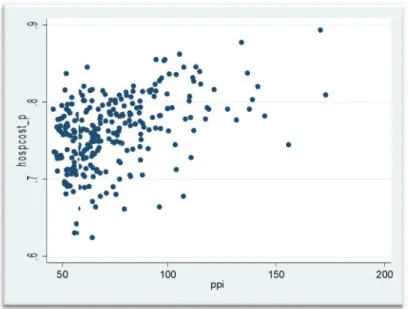
In the graph number 1 we can see that, apparently the correlation between relative hospital expenditure (y axis) and the purchasing power (x axis) exists and it is positive in the sense that an increase in the ppi generally leads to an increase in the share of hospital expenditure, but we must check whether this relation is also supported by econometric analysis (relations with other explanatory variables is in Appendix 2).

Graph 1 – Relation between percentage of Hospital expenditure (hospcost_p) and purchasing power parity (ppi)

docs 281 1.743416 2.221398 0 25.9 surg_ind 281 1.016313 .132889 .6487997 1.761683 famdoc_p 281 .8880356 .0991167 .5963778 .9963292 fempop_p 281 51.38996 .7557346 49.47 54.9 popdens 281 296.3801 771.5949 5.3 7183.3 ppiTyouth_~d 281 1581.594 626.4084 624.118 3995.145 ppiTeld_ind 281 2482.95 762.2876 880.739 5404.85 youth_ind 281 20.75409 3.065789 11.6 27.6 eld_ind 281 34.63701 11.57042 14.9 80.8 ppiTcol_dgr 281 430.6568 458.2548 0 3920.776 col_dgr 281 4.981744 2.993603 0 22.67 ppi 281 74.88886 23.13226 45.88 172.95

Variable Obs Mean Std. Dev. Min Max

. su ppi col_dgr ppiTcol_dgr eld_ind youth_ind ppiTeld_ind ppiTyouth_ind popdens fempop_p famdoc_p surg_ind docs In table 1 we can see some descriptive statistics of the explanatory variables in the

regression, including means, standard deviations, minimum and maximum values.

4. Results

. su ppi col_dgr ppiTcol_dgr eld_ind youth_ind ppiTeld_ind ppiTyouth_ind popdens fempop_p famdoc_p surg_ind docs In table 1 we can see some descriptive statistics of the explanatory variables in the

regression, including means, standard deviations, minimum and maximum values.

4. Results

(20)

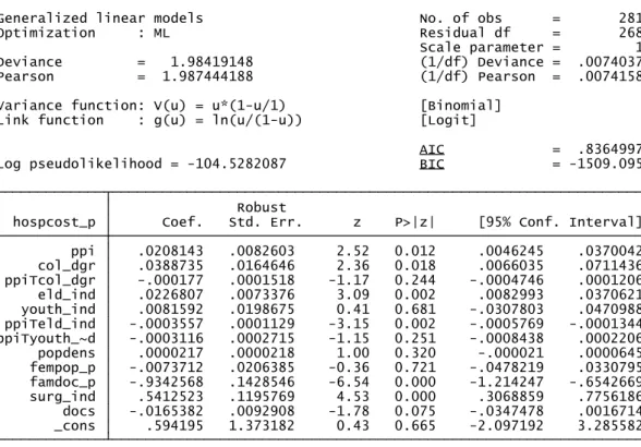
Below we can see the Stata output of the regression presented in the end of previous section using the Quasi-Likelihood method already described:

Table 2 – Regression using Quasi-Likelihood method1

The output above shows us several variables appear to not be statistically significant, namely the interaction term between purchasing power and college degree, the percentage of female population, population density, the variables relating to the youth index and the number of doctors per 1000 inhabitants. This means that either they don’t affect public health care expenditure at all, or, if they do, they don’t it with a bias towards hospitals or primary care centers.

Our main variable of interest, ppi, presents a p-value close to 1%. Furthermore, the sign of the coefficient is the one we expected. According to this regression, counties with more purchasing power also have bigger slice of health care expenditure devoted

_cons .594195 1.373182 0.43 0.665 -2.097192 3.285582 docs -.0165382 .0092908 -1.78 0.075 -.0347478 .0016714 surg_ind .5412523 .1195769 4.53 0.000 .3068859 .7756186 famdoc_p -.9342568 .1428546 -6.54 0.000 -1.214247 -.6542669 fempop_p -.0073712 .0206385 -0.36 0.721 -.0478219 .0330795 popdens .0000217 .0000218 1.00 0.320 -.000021 .0000645 ppiTyouth_~d -.0003116 .0002715 -1.15 0.251 -.0008438 .0002206 ppiTeld_ind -.0003557 .0001129 -3.15 0.002 -.0005769 -.0001344 youth_ind .0081592 .0198675 0.41 0.681 -.0307803 .0470988 eld_ind .0226807 .0073376 3.09 0.002 .0082993 .0370621 ppiTcol_dgr -.000177 .0001518 -1.17 0.244 -.0004746 .0001206 col_dgr .0388735 .0164646 2.36 0.018 .0066035 .0711436 ppi .0208143 .0082603 2.52 0.012 .0046245 .0370042 hospcost_p Coef. Std. Err. z P>|z| [95% Conf. Interval]

Robust

Log pseudolikelihood = -104.5282087 BIC = -1509.095

AIC = .8364997

Link function : g(u) = ln(u/(1-u)) [Logit] Variance function: V(u) = u*(1-u/1) [Binomial]

Pearson = 1.987444188 (1/df) Pearson = .0074158

Deviance = 1.98419148 (1/df) Deviance = .0074037

Scale parameter = 1

Optimization : ML Residual df = 268

(21)

to the hospital. The variable associated with the percentage of population with tertiary education (col_dgr) also shows a positive coefficient.

Despite the failure of the weight of the younger population in explaining the dependent variable, the same doesn’t happen when we take into account the elderly. Both coefficients related with the elderly index are highly significant. Even though the coefficient for this eld_ind is positive, we must take into account that the marginal effect of this variable must always take into account the variable ppiTeld_ind, and that this marginal effect will depend on the level of ppi. Thus, since the sign of this second term is negative, there will be a level of ppi for which the marginal effect of the relative number of elderly people will start to be negative.

As for the percentage of population with family doctor (famdoc_p), we can see that the sign of the coefficient also makes perfect sense. An increase in the percentage of population with family doctor is expected to lead to a diminishing share of relative hospital expenditure. This is simply explained by two factors: first due to a strong preference in seeing the respective family doctor whenever possible as normally there is a relationship of greater trust than with a new doctor; the second is the fact that this variable also serves as a measure of supply capacity of the PCC, which, as we know, can serve as a repulsive factor for the population if demand is chronically unsatisfied with the service rendered.

Finally, the surgery index is highly significant as well, as expected. This control variable, like we have mentioned before, is included to capture the effect of asymmetries in surgeries that occur across counties and that inflate the hospital expenditure, without being a consequence of the choices of the NHS users at all. Once again it presents the reasonable sign, with counties with a more elevated figure for this index registering an increase in relative hospital expenditure.

(22)

For comparison purposes, we also ran a simple OLS regression with robust standard errors using the exact same dependent variable and regressors. Surprisingly, or maybe not, no changes whatsoever occurred from the Quasi-Likelihood model both in terms of significance of the variables and in terms of the sign of the coefficients. The output related to the aforementioned regression is below in table 3.

Table 3 – Simple Linear regression

The accurate marginal effects of each variable that we find in the first regression will evidently not be constant due to the type of underlying model that we are using. However, given the robustness shown by the OLS estimate concerning significance and sign of coefficients, we can safely assume that the scale of the coefficients computed by OLS will be close to the real values for cases close to the mean. This is useful because it allows for a more intuitive interpretation of the magnitude that a change in one of our independent variables will have on relative hospital expenditure. Furthermore, given that the simple average of total expenditure in our database reaches the 24.5€ million

_consdocs -.0029392.6758449 .2465629.0015818 -1.862.74 0.0070.064 -.0060536.1903984 1.161291.0001752 surg_ind .0996437 .0223231 4.46 0.000 .0556927 .1435947 famdoc_p -.1647832 .0255504 -6.45 0.000 -.2150881 -.1144782 fempop_ppopdens -.00160342.46e-06 3.44e-06.003742 -0.430.71 0.6690.476 -.0089709-4.31e-06 9.23e-06.005764 ppiTyouth_~d -.0000497 .0000474 -1.05 0.295 -.000143 .0000436 ppiTeld_ind -.000064 .0000199 -3.21 0.001 -.0001032 -.0000247 youth_indeld_ind .0010401.0040752 .0035563.0013058 0.293.12 0.7700.002 -.0059617.0015042 .0080418.0066462 ppiTcol_dgr -.0000365 .0000236 -1.55 0.122 -.0000829 9.88e-06 col_dgr .0074813 .0028207 2.65 0.008 .0019278 .0130348 ppi .0036173 .0014339 2.52 0.012 .0007941 .0064404 hospcost_p Coef. Std. Err. t P>|t| [95% Conf. Interval]

Robust

Root MSE = .03681 R-squared = 0.3754 Prob > F = 0.0000 F( 12, 268) = 14.48

(23)

into a 245.000€ shift to hospital expenditure from PCC, on average. This can be used as an important tool to assess the economic significance of the results.

For example, if we look at the coefficient for ppi we see that an increase in one point of this index leads to an increase of over 0.3 p.p. in our dependent variable. Given that the purchasing power index varies from close to 50 to close to 170 points, being 100 the national average, the difference in the corresponding predicted values amounts to 36%, ceteris paribus. In monetary terms, we can infer that these 0.3% increases in the dependent variable, caused by a one point increment in the ppi, translate into 73.500€, on average. The regression shows that the elderly index will also influence this marginal effect through the variable ppiTeld_ind which is significant. However the coefficient associated is not very large (-.000064), so it should only slightly affect the discussed impact of ppi and for counties with large percentage of elderly.

Similarly, for the percentage of population with college degree, we see that an increase in a single percentage point in this variable can lead, on average, to an impact of 0.748 p.p. in hospcost_p. Once again, translating this into euros, we get a figure close to 180.000€.

It is also worth mentioning the effect that the percentage of population with family doctor in their respective primary care center (measured between 0 and 1) has in this regression (as it can be influenced in the relative short term by policy decisions), with a variation of one percentage point implying a change of 0.16% in our dependent variable. This highlights the importance of assigning a family doctor in determining a greater level of Primary care center demand, which can be very important if, for example, the Hospitals of a given region have chronic problems in satisfying demand.

Due to the economic situation faced in Portugal that threatens to impoverish a considerable part of its population, it is also interesting to analyze these results in that

(24)

light. If we assume that the result that we found comparing different regions also occurs across time and that it is possible for it to be reversed we can also predict a future downward trend in the share of expenditure devoted to hospital care. Quantifying, a decrease of 10 points in purchasing power from the level in 2009, could lead to a predicted drop of 3.6 percentage points in our dependent variable in each county (over 830.000€, on average, using our estimates). If efforts to increase percentage of population with family doctors are taken, this change can be even more drastic. By our figures, an increase of only 5% from the 88.8% of current coverage of family doctors could mean an extra 0.8% in our dependent variable. It is worth mentioning however that these estimates are likely over estimated because marginal effect will not be as strong as we move away from the mean. Furthermore, in the case of family doctors, population that does not have one tends to need less health care, so the impact in aggregate expenditure may not be as large.

5. Conclusions

In this work project we set out to study the potential impact of socioeconomic factors in the choice made by the user of the Portuguese NHS between Hospital and primary care center. With that purpose we used information on Hospital expenditure and Primary care center cost per county for the year of 2009 as well as socio-demographic data on the population. This information was provided by the Portuguese administration of the NHS (ACSS) or mostly acquired in through the database of the Portuguese statistics institute (INE).

The model that we used for the analysis attempted to explain disparities in the percentage of health care expenditure devoted to hospitals, given by the hospital expenditure divided by the sum of aggregate primary center expenditure plus hospital

(25)

expenditure. It was found this was the best alternative to capture the effect that we are looking for, given the data available, since we expect that if there is a general preference for richer people to go to the hospital, then in richer areas we should, on average, encounter a higher share of relative hospital expenditure since the demand will tend to be larger. We used a Quasi-Likelihood method, like the one proposed by Papke and Wooldridge to estimate the regression since we are in the presence of a fractional response variable, though OLS results seem to be quite robust.

In the end we found that both purchasing power and tertiary education have explanatory power in relation to our dependent variable and both with considerable magnitude and the expected positive sign. Theoretical reasons put forward for this are linked with different perceptions of severity when dealing with health care conditions and a greater ease in dealing with hospital bureaucracies.

These findings can be helpful in guiding policy decisions in relation to Portuguese primary care. During the elaboration of this work project, news about a new policy allowing Hospitals to refer patients to Primary care centers if they find the severity of the condition does not require hospital assistance. What we have found here points to the fact that the impact that this may have across different regions of the country in terms of a potential surge in primary care center demand is likely to be heterogeneous. Areas with higher income have to be prepared for larger surge of referrals and resources must be managed accordingly

If this measure is implemented it is likely that data about referrals might be gathered. If this happens, it would allow for a much more detailed analysis of the problem, begging a revisiting of the topic to confirm or contradict the results that we obtained.

(26)

6. References

Per Rosen, Anders Anell and Catharina Hjortsberg, “Patient views on choice and

participation in primary health care”, Health Policy, 2001, vol. 55, issue 2, pages 121-128

Papke, Leslie E & Wooldridge, Jeffrey M, (1996), "Econometric Methods for Fractional

Response Variables with an Application to 401(K) Plan Participation Rates", Journal of

Applied Econometrics, John Wiley & Sons, Ltd., vol. 11(6), pages 619-32, Nov.-Dec. Duan N. (1983), “Smearing estimate: a nonparametric retransformation method”, Journal of the American Statistical Association 1983; 78:605-610.

Gourieroux, Christian & Monfort, Alain & Trognon, Alain, 1984. "Pseudo Maximum

Likelihood Methods: Theory" Econometrica, Econometric Society, vol. 52(3), pages 681-700,

May

Tudor Hart, J. (1971), "The Inverse Care Law", The Lancet 297: 405–412

Pell JP, Pell AC, Norrie J, et al, BMJ. 2000, “Effect of socioeconomic deprivation on

waiting time for cardiac surgery: retrospective cohort study”, BMJ 2000;320:15–8. 24

António G. Rodrigues, Paula Santana, Rita Santos, Helena Nogueira, “Optimização da

Rede das Unidades Básicas de Urgência em Portugal Continental: Uma metodologia para a Reorganização Espacial da Capacidade Instalada”

OECD Health Data 2011

Defining Primary Care: An Interim Report (IOM, 1994b)

Portarias nº 272 through 276/2009 of March 18th_{, Diário da República}

(27)

Appendix 1 – List of GDH excluded from the analysis (in Portuguese)

GDH Designação

GCD 14 Gravidez, Parto e Puerpério

370 Cesariana, com CC 371 Cesariana, sem CC

372 Parto vaginal, com diagnósticos de complicação 373 Parto vaginal, sem diagnósticos de complicação 374 Parto vaginal, com esterilização e/ou dilatação e/ou_curetagem 375 Parto vaginal, com procedimento em BO, excepto_{esterilização e/ou dilatação e/ou curetagem uterina} 376 Diagnósticos pós-parto e/ou pós-aborto, sem procedimento_{em B.O.} 377 Diagnósticos pós-parto e/ou pós-aborto, com procedimento_{em B.O.} 378 Gravidez ectópica

379 Ameaça de abortamento

380 Abortamento, sem dilatação e curetagem

381 Abortamento com dilatação e/ou curetagem, curetagem de_{aspiração e/ou histerotomia} 382 Falso trabalho de parto

383 Outros diagnósticos pré-parto, com complicações médicas 384 Outros diagnósticos pré-parto, sem complicações médicas 650 Cesariana de alto risco, com CC

651 Cesariana de alto risco, sem CC

652 Parto vaginal de alto risco, com esterilização e/ou dilatação_{e/ou curetagem uterina}

GCD 20 Uso de Álcool/Droga e Perturbações Mentais Orgânicas_{Induzidas por Álcool ou Droga}

743 Abuso ou dependência de opiáceos, alta contra parecer_médico 744 Abuso ou dependência de opiáceos, com CC 745 Abuso ou dependência de opiáceos, sem CC

746 Abuso ou dependência de cocaína ou de outras drogas, alta_{contra parecer médico} 747 Abuso ou dependência de cocaína ou de outras drogas, com_CC 748 Abuso ou dependência de cocaína ou de outras drogas, sem_CC 749 Abuso ou dependência do álcool, alta contra parecer médico 750 Abuso ou dependência do álcool, com CC

(28)

GCD 22 Queimaduras

821 Queimaduras extensas, de 3º grau, com enxerto de pele 822 Queimaduras extensas, de 3º grau, sem enxerto de pele 823 Queimadura da espessura total da pele, com enxerto da pele_{ou lesão de inalação, com CC ou traumatismos significativos} 824 Queimadura da espessura total da pele, com enxerto da pele_{ou lesão de inalação, sem CC ou traumatismos significativos} 825 Queimadura da espessura total da pele, sem enxerto da pele_{ou lesão de inalação, com CC ou traumatismos significativos} 826 Queimadura da espessura total da pele, sem enxerto da pele_{ou lesão de inalação, sem CC ou traumatismos significativos} 827 Queimaduras não extensas, com lesão de inalação, CC ou_{traumatismos significativos} 828 Queimaduras não extensas, sem lesão de inalação, CC ou_{traumatismos significativos}

GCD 25 Traumatismos Múltiplos Significativos

730 Craniotomia por traumatismos múltiplos significativos 731 Procedimentos na coluna, anca, fémur e/ou membro, por_{traumatismos múltiplos significativos} 732 Outros procedimentos em B.O., por traumatismos múltiplos_{significativos} 733 Diagnósticos de traumatismos múltiplos significativos da_{cabeça, tórax e/ou membros inferiores} 734 Outros diagnósticos de traumatismos múltiplos significativos 792 Craniotomia por traumatismos múltiplos significativos, com_{CC major não traumáticas} 793 Procedimentos por traumatismos múltiplos significativos,_{excepto craniotomia, com CC major não traumáticas} 794 Diagnósticos de traumatismos múltiplos significativos, com_{CC major não traumáticas}

GCD 0 (Pré-Grandes Categorias Diagnósticas)

103 Transplante cardíaco 302 Transplante renal 480 Transplante hepático

482 Traqueostomia por diagnósticos da face, boca e/ou pescoço 483 Oxigenação por membrana extra-corporal, traqueostomiacom ventilação mecânica >96h ou traqueostomia com outro diagnóstico principal, excepto da face, boca ou do pescoço 795 Transplante de pulmão

803 Transplante alogénico de medula óssea 804 Transplante autólogo de medula óssea 805 Transplante simultâneo de rim e de pâncreas 829 Transplante de pâncreas

(29)

.6 5 .7 .7 5 .8 .8 5 .9 ho sp co st _p 0 5 10 15 20 25 col_dgr .6 5 .7 .7 5 .8 .8 5 .9 ho sp co st _p 50 100 150 200 ppi .6 5 .7 .7 5 .8 .8 5 .9 ho sp co st _p 0 1000 2000 3000 4000 ppiTcol_dgr .6 5 .7 .7 5 .8 .8 5 .9 ho sp co st _p 20 40 60 80 eld_ind .6 5 .7 .7 5 .8 .8 5 .9 ho sp co st _p 10 15 20 25 30 Youth_ind .6 5 .7 .7 5 .8 .8 5 .9 ho sp co st _p 1000 2000 3000 4000 5000 ppiTeld_ind

Appendix 2 – Graphic relation between independent (hospcost_p) and dependent variables

2.1. ppi 2.2. col_dgr

2.3. ppiTcol_dgr 2.4. eld_ind

(30)

.6 5 .7 .7 5 .8 .8 5 .9 ho sp co st _p 0 1000 2000 3000 4000 ppiTyouth_ind .6 5 .7 .7 5 .8 .8 5 .9 ho sp co st _p 0 2000 4000 6000 8000 popdens .6 5 .7 .7 5 .8 .8 5 .9 ho sp co st _p 48 50 52 54 56 fempop_p .6 5 .7 .7 5 .8 .8 5 .9 ho sp co st _p .6 .7 .8 .9 1 famdoc_p .6 5 .7 .7 5 .8 .8 5 .9 ho sp co st _p .5 1 1.5 2 surg_ind .6 5 .7 .7 5 .8 .8 5 .9 ho sp co st _p 0 5 10 15 20 25 Docs 2.7. ppiTyouth_ind 2.8. popdens 2.9.fempop_p 2.10. famdoc 2.11. surg_ind 2.12. docs

(31)

d o c s 0 . 2 4 4 3 0 . 6 1 7 6 0 . 7 1 6 5 0 . 7 5 5 3 -0 . 2 0 8 4 0 . 1 0 7 0 0 . 3 3 7 8 0 . 5 1 6 6 0 . 3 8 4 1 0 . 3 0 5 2 -0 . 0 6 7 7 0 . 2 2 8 8 1 . 0 0 0 0 s u r g _ i n d 0 . 1 4 5 8 0 . 0 4 6 4 0 . 0 4 1 4 0 . 0 7 0 3 0 . 3 5 0 1 -0 . 3 6 9 7 0 . 4 0 4 3 -0 . 1 0 0 4 -0 . 0 2 4 5 0 . 2 8 6 2 0 . 3 6 7 0 1 . 0 0 0 0 f a m d o c _ p -0 . 3 5 3 0 -0 . 3 4 7 4 -0 . 2 5 0 0 -0 . 2 7 2 8 0 . 3 0 2 8 -0 . 3 9 4 8 -0 . 0 1 2 7 -0 . 4 2 6 2 -0 . 2 9 5 6 0 . 3 4 5 9 1 . 0 0 0 0 f e m p o p _ p -0 . 0 6 2 2 -0 . 0 3 0 0 0 . 1 6 5 5 0 . 1 8 3 3 0 . 1 5 8 2 -0 . 2 4 7 3 0 . 1 0 5 7 -0 . 0 9 0 3 0 . 1 8 4 2 1 . 0 0 0 0 p o p d e n s 0 . 3 2 1 5 0 . 5 1 1 9 0 . 5 2 8 8 0 . 5 7 3 1 -0 . 3 0 6 7 0 . 2 1 7 7 0 . 1 1 6 2 0 . 4 8 5 8 1 . 0 0 0 0 p p i T y o u t h _ ~ d 0 . 3 9 1 0 0 . 9 4 4 5 0 . 7 8 2 7 0 . 8 1 2 5 -0 . 5 3 9 8 0 . 6 5 3 3 0 . 3 0 0 9 1 . 0 0 0 0 p p i T e l d _ i n d 0 . 2 4 6 8 0 . 4 7 2 9 0 . 3 6 5 8 0 . 4 3 3 5 0 . 5 8 5 2 -0 . 2 7 8 4 1 . 0 0 0 0 y o u t h _ i n d 0 . 0 5 9 9 0 . 3 8 6 9 0 . 3 0 0 7 0 . 2 8 8 4 -0 . 6 5 3 5 1 . 0 0 0 0 e l d _ i n d -0 . 1 2 2 4 -0 . 4 1 6 1 -0 . 3 6 3 9 -0 . 3 2 4 7 1 . 0 0 0 0 p p i T c o l _ d g r 0 . 4 0 7 2 0 . 8 7 2 8 0 . 9 6 1 7 1 . 0 0 0 0 c o l _ d g r 0 . 4 0 8 9 0 . 8 3 4 5 1 . 0 0 0 0 p p i 0 . 4 5 1 2 1 . 0 0 0 0 h o s p c o s t _ p 1 . 0 0 0 0 h o s p c o ~ p p p i c o l _ d g r p p i T c o ~ r e l d _ i n d y o u t h _ ~ d p p i T e l ~ d p p i T y o ~ d p o p d e n s f e m p o p _ p f a m d o c _ p s u r g _ i n d d o c s