FACULDADE DE
ENGENHARIA DA
UNIVERSIDADE DO
PORTO
Data analysis of the flow over Serra do
Perdigão based on the sonic flow
anemometers
Nuno Vieira Cardoso
MSc in Mechanical Engineering
Supervisor: José Manuel Laginha Mestre da Palma
c
Data analysis of the flow over Serra do Perdigão based on
the sonic flow anemometers
Nuno Vieira Cardoso
MSc in Mechanical Engineering
Resumo
A campanha de medições da Serra do Perdigão ocorreu entre Dezembro de 2016 e Junho 2017 e o seu objectivo foi adquirir dados sobre a influência exercida por duas colinas sobre o escoamento atmosférico. O local foi escolhido para estudar o vento sobre uma colina e verificar a separação do escoamento e a recirculação a jusante da colina e no vale. A Serra do Perdigão tem duas colinas o que se revela mais vantajoso para o estudo porque o escoamento a jusante da primeira colina é o mesmo que o escoamento a montante da segunda colina.
Um grande conjunto de sensores foram colocados nas torres meteorológicas, com alturas entre os 10 e os 100 metros, distribuídas pelo vale, pelas colinas, e por duas linhas perpendiculares às colinas. Os dados recolhidos pelos anemómetros sónicos das torres permitiram estudar as carac-terísticas do escoamento (parâmetros). Estes dados foram comparados com simulações que tinham sido feitas usando diferentes modelos de rugosidade da superfície. O escoamento no vale é per-pendicular às duas colinas e existem zonas de recirculação a jusante das colinas. Os parâmetros do escoamento foram estudados para dois grupos de direcção do vento: Nordeste e Sudoeste. Para os dois grupos observou-se separação do escoamento no topo das colinas e zonas de recirculação a jusante das colinas. Os resultados das simulações feitas anteriormente são uma boa aproximação das medições de campo realizadas na Serra do Perdigão.
Abstract
The Perdigão Field experiment took place from December 2016 to June 2017 and its aim was to collect data regarding the influence exerted by an uphill stream with flow separation on the wind speed and turbulence. It was chosen to measure wind resources along a ridge, occurrences of flow separation on lee-sides of hills and valley flows. Perdigão has a double ridge in comparison to a single-ridge site and provides a list of additional advantages because the lee-side flow is also the flow impinging on the second ridge.
A large array of sensors were located on meteorological towers, 10 to 100 m high, distributed along the valley, the SW and NE ridges, and two transect lines perpendicular to the ridges. The data of the sonic anemometers of the towers allowed the flow parameters to be analysed and reveal the flow patterns. The measurements done on the field were compared with the flow simulations that were made using different surface cover models. The measurements showed the same patterns than the flow simulation. The flow in the valley is perpendicular to both ridges and there are zones of re-circulation in the valley on the lee side of the first-ridge. The flow patterns were studied for two groups of wind direction: Northeast winds and Southwest winds. For both directions (NE and SW) the flow separation occurred at the peak of both ridges and on the lee-side of the hills there was re-circulation of the flow. The flow simulations to study the flow parameters that were done previously using different surface cover models are in accordance with the data collected from the sonic anemometers showing similar values and behaviour of the flow parameters.
Acknowledgements
I would like to thank Prof. Laginha for his supervision.
I want to thank my father and my brother for their unwavering support.
Nuno Cardoso
Hard work pays off
Contents
1 Introduction 1
1.1 NEWA . . . 1
1.2 Site description . . . 1
1.3 Perdigão field experiment . . . 2
1.4 Measurement periods and contributors . . . 3
1.5 Flow over a Hill . . . 3
1.6 Outline of the thesis . . . 4
2 Methodology 5 2.1 Data . . . 5 2.2 100 m towers . . . 7 2.3 60 m towers . . . 9 2.4 30 m towers . . . 10 2.5 20 m towers . . . 12 2.6 10 m towers . . . 13
2.7 Flow over Serra do Perdigão . . . 14
3 Results and discussion 17 3.1 Northeast winds . . . 17 3.1.1 10 meters a.g.l. . . 18 3.1.2 20 meters a.g.l. . . 21 3.1.3 30 meters a.g.l. . . 24 3.2 Southwest Winds . . . 27 3.2.1 10 meters a.g.l. . . 27 3.2.2 20 meters a.g.l. . . 30 3.2.3 30 meters a.g.l. . . 33
3.3 Comparison with flow simulation . . . 36
3.3.1 Northeast winds . . . 36
3.3.2 Southwest winds . . . 39
4 Conclusions and future work 43 4.1 Conclusions . . . 43
4.2 Northeast winds . . . 43
4.3 Southwest winds . . . 44
4.4 Future work . . . 44
References 45
A Contour maps data 47
x CONTENTS
B Python scripts 61
List of Figures
1.1 Terrain and tower layout of the Perdigão 2017 campaign. . . 2
1.2 Flow over a isolated hill . . . 3
2.1 Pressure variation at 2 meters in four towers. . . 6
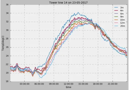
2.2 Temperature variation at tower tnw14 on May 23rd at different heights. . . 6
2.3 Towers 20, 25 and 29 in serra do Perdigão. . . 7
2.4 Wind speed averages variation with height during IOP. . . 9
2.5 Locations of the 60 m towers. . . 10
2.6 Towers with 30 m in serra do Perdigão. . . 11
2.7 Towers with 20 m in serra do Perdigão. . . 12
2.8 Towers with 10m in serra do Perdigão. . . 13
3.1 horizontal wind speed (m/s) at 10 meters a.g.l . . . 18
3.2 Velocity component u at 10 meters a.g.l (m/s) . . . 19
3.3 Velocity component v at 10 meters a.g.l (m/s) . . . 19
3.4 Velocity component w at 10 meters a.g.l (m/s) . . . 20
3.5 Turbulent kinetic energy at 10 meters a.g.l . . . 20
3.6 Horizontal speed at 20 meters a.g.l (m/s) . . . 21
3.7 Horizontal speed at 20 meters a.g.l. (m/s) . . . 22
3.8 Velocity component v (cross-stream) at 20 meters a.g.l. (m/s) . . . 22
3.9 Velocity component w (vertical) at 20 meters a.g.l. (m/s) . . . 23
3.10 Turbulent kinetic energy at 20 meters a.g.l . . . 23
3.11 Horizontal speed at 30 meters a.g.l. (m/s) . . . 24
3.12 Velocity component u (stream-wise) at 30 meters a.g.l. (m/s) . . . 25
3.13 Velocity component v (stream-wise) at 30 meters a.g.l. (m/s) . . . 25
3.14 Velocity component v (stream-wise) at 30 meters a.g.l. (m/s) . . . 26
3.15 Turbulent kinetic energy at 30 meters a.g.l . . . 26
3.16 Horizontal speed at 10 meters a.g.l. (m/s) . . . 28
3.17 Velocity component u (stream-wise) at 10 meters a.g.l. (m/s) . . . 28
3.18 Velocity component v (cross-stream) at 10 meters a.g.l. (m/s) . . . 29
3.19 Velocity component w (vertical) at 10 meters a.g.l. (m/s) . . . 29
3.20 Turbulent kinetic energy at 10 meters a.g.l . . . 30
3.21 Horizontal speed at 20 meters a.g.l. (m/s) . . . 31
3.22 Velocity component u (stream-wise) at 20 meters a.g.l. (m/s) . . . 31
3.23 Velocity component v (cross-stream) at 20 meters a.g.l. (m/s) . . . 32
3.24 Velocity component w (vertical) at 20 meters a.g.l. (m/s) . . . 32
3.25 Turbulent kinetic energy at 20 meters a.g.l. . . 33
3.26 Horizontal speed at 30 meters a.g.l. (m/s) . . . 34
xii LIST OF FIGURES
3.27 Velocity component u (stream-wise) at 30 meters a.g.l. (m/s) . . . 34
3.28 Velocity component v (cross-stream) at 30 meters a.g.l. (m/s) . . . 35
3.29 Velocity component w (vertical) at 30 meters a.g.l. (m/s) . . . 35
3.30 Turbulent kinetic energy at 30 meters a.g.l . . . 36
3.31 Flow simulation for NE winds for tower 20 . . . 37
3.32 Flow simulation for NE winds for tower 37 . . . 37
3.33 Flow simulation for NE winds for tower 29 . . . 38
3.34 Flow simulation for NE winds for tower 25 . . . 38
3.35 Flow simulation for SW winds for tower 20 . . . 39
3.36 Flow simulation for SW winds for tower 37 . . . 40
3.37 Flow simulation for SW winds for tower 20 . . . 40
3.38 Flow simulation for SW winds for tower 29 . . . 41
3.39 Flow simulation for SW winds for tower 25 . . . 41
C.1 Tower 29 NE winds v component at 60 meters a.g.l. . . 65
C.2 Tower 7 NE winds v component at 60 meters a.g.l. . . 66
List of Tables
2.1 Wind speed at 100 m towers . . . 8
2.2 Locations of the 60 m towers . . . 9
2.3 Locations of the 30 m towers . . . 10
2.4 Locations of the 20 m towers . . . 13
2.5 Locations of the 10 m towers . . . 14
A.1 Horizontal speed at 10 meters a.g.l. . . 48
A.2 Velocity component u (stream-wise) at 10 meters a.g.l. . . 49
A.3 Velocity component v (cross-stream) at 10 meters a.g.l. . . 50
A.4 Velocity component w (vertical) at 10 meters a.g.l. . . 51
A.5 Turbulent kinetic energy at 10 meters-high anemometers . . . 52
A.6 Horizontal speed at 20 meters a.g.l. . . 53
A.7 Velocity component u (stream-wise) at 20 meters a.g.l. . . 54
A.8 Velocity component v (cross-stream) at 20 meters a.g.l. . . 55
A.9 Velocity component w (vertical) at 20 meters a.g.l. . . 56
A.10 Turbulent kinetic energy at 20 meters-high anemometers . . . 57
A.11 Horizontal speed at 30 meters a.g.l. . . 58
A.12 Velocity component u (stream-wise) at 30 meters a.g.l. . . 58
A.13 Velocity component v (cross-stream) at 30 meters a.g.l. . . 59
A.14 Velocity component w (vertical) at 30 meters a.g.l. . . 59
A.15 Turbulent kinetic energy at 30 meters-high anemometers . . . 60
Abbreviations and Symbols
EMP Extensive measurement period IOP Intensive observational period a.g.l. Above ground level
NEWA New European Wind Atlas NetCDF Network Common Data Form spd horizontal speed
u stream-wise velocity component v cross-stream velocity component w vertical velocity component TKE Turbulent Kinetic energy
Chapter 1
Introduction
1.1
NEWA
The New European Wind Atlas (NEWA) is a project concerned with:
• creation of a freely accessible wind atlas covering the European Union, Turkey and Euro-pean coastal water within 100 km off the shore. The main content of the atlas is site-specific wind resources, but also extreme winds, turbulence, shear and other parameters relevant for wind turbine siting will be included.;
• development of models or a model chain to produce the high-resolution wind atlas;
• atmospheric flow experiments in various kinds of complex terrain to validate the mod-els. (Mann et al.,2017)
The NEWA project aims to improve wind resource modeling for different site conditions. Areas with steep ridges and forested terrain are of particular interests since the current engineering (linear) flow models are unable to correctly predict the behavior of the flow over the sites with these features. The Perdigão field experiment is one of the experiments included in this project.
1.2
Site description
Perdigão is formed by two parallel ridges, with southeast–northwest orientation and the dis-tance between them around 1.4 km, that measure about 4 km lengthwise and are 500–550 m above sea level (a.s.l.) at their summits. The valley-to-peak height is about 200 to 250 m and the hills are steep, with an inclination of approximately 35 percent. A double ridge in comparison to a single-ridge site provides a list of additional advantages because the lee-side flow is also the flow impinging on the second ridge. Furthermore, the lee side of the first hill and the upwind side of the second hill make up the valley flow. The terrain coverage is irregular, made of no or low-height vegetation and patches of eucalyptus and pine trees (Vasiljevic et al.,2017).
2 Introduction
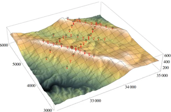
Figure 1.1: Terrain and tower layout of the Perdigão 2017 campaign. (Mann et al.,2017)
The predominant winds were from the northeast and west–southwest directions, i.e., perpen-dicular to the ridges, with a mean and maximum wind speed of around 6 and 20 m/s respec-tively (Vasiljevic et al.,2017). These directions are also those with highest average velocity and lowest levels of turbulent intensity.
1.3
Perdigão field experiment
The Perdigão Field experiment aim was to study and acquire data regarding the influence exerted by an uphill stream with flow separation on the wind speed and turbulence. To assist the NEWA project, it was chosen to measure wind flow along a ridge, occurrences of flow separations on lee sides of hills (i.e. re-circulation zone) and valley flows.
A large array of sensors were located on meteorological towers, 10 to 100 m high, distributed along the valley, the SW and NE ridges, and two transect lines perpendicular to the ridges. Re-mote sensing equipment provided additional information, both within this area increasing the height range and via scanning patterns on planes perpendicular or aligned with the ridges, for a three-dimensional view of the wind flow pattern within and both upstream and downstream of the site (Mann et al.,2017).
The meteorological towers carried a total of 195 three-component sonic anemometers, 55 tem-perature–humidity sensors, 22 barometers, 8 microbarometers, 14 radiometers, 17 CO2/H2O gas analyzers,13 wetness sensors, 16 heat/moisture flux sensors, 5 thermohygrometers, and 3 pyrge-ometers. The instruments were mounted at heights 2, 10, 20, 30, 40, 60, 80, and 100 m above ground level (a.g.l.), depending on instrument availability and science needs. All towers recorded
1.4 Measurement periods and contributors 3 at 20 Hz the local mean velocity, turbulence, heat, and momentum fluxes using sonic anemometers to help process and modeling studies. A subset of 16 of the towers directly measured all terms of the surface energy balance (flux towers) (Fernando et al.,2019).
1.4
Measurement periods and contributors
The Perdigão Intensive Observational Period (IOP) took place from 1 May to 15 June 2017 in the Serra do Perdigão area to the southwest of Castelo Branco, Portugal. There was an extensive network of towers and scanning and profiling lidars along with a set of in-situ and remote sensing profiling instrumentation from US (University of Notre Dame, University of Colorado-Boulder, University of Oklahoma, NCAR/EOL, Cornell University, University of California-Berkeley and the Army Research Laboratory) as well as European (DTU, University of Porto, DLR, ForWinds, ENERCON, WindForS, NCAS) groups. There was also a longer term Extensive Measurements Period (EMP) that took place from 15 December 2016 to 3 July 2017 with a subset of the instru-mentation. Only the measurements done in the IOP will be the aim of this work.
1.5
Flow over a Hill
The pattern of airflow around a hill is determined not only by the hill shape but also by its size. The vertical movement of air parcels that must occur as the wind flows over a hill is accompanied by a gravitational restoring force. The flow over complex terrain is usually associated to flow sepa-ration, high shear factors and turbulence levels. In a simplified hill topography the flow accelerates to the top where it reaches maximum velocity and, for steep hills, can separate yielding a highly turbulent wake region downstream. The changes in surface elevation can alter the pressure field of the hill region, which affect the local flow field (Kaimal and Finnigan,1994).
4 Introduction
1.6
Outline of the thesis
This dissertation is divided into four chapters. Chapter1, coming to an end, gives a general view of the field experiment and its purpose. The methodology is covered on chapter2and the discussion of the results is on chapter3. Chapter4is where are the conclusions and suggestions for future works. AppendixAcontains the measurements data for the IOP used to plot the contour maps. Appendix B contains the python scripts that were used to handle the data sets and an example of a script that was used to make the contour plots.
Chapter 2
Methodology
The present chapter describes how the data of the Perdigão field experiment was handled and the software that was used to process the data collected in section2.1. The coordinates of the towers are presented in sections2.2,2.3,2.4,2.5and2.6. In section2.7is described the flow parameters that are going to be analysed and how the results of the measurements will be presented and divided in two groups that follow a criteria.
2.1
Data
The data from Perdigão was uploaded and stored on NetCDF files. NetCDF (Network Com-mon Data Form) is a set of interfaces for array-oriented data access and a freely distributed collec-tion of data access libraries for C, Fortran, C++, Java, and other languages. The NetCDF libraries support a machine-independent format for representing scientific data. Together, the interfaces, libraries, and format support the creation, access, and sharing of scientific data.
In this work, python was the language used to access the data collected from the Perdigão field campaign. To open and read the files in python a package called xarray was used to visualize and convert the data sets into data frames (two-dimensional tabular data structure with row and column labels). After this conversion, the data stored in the data frame was processed using another python package called pandas. For data visualisation a package called matplotlib was used in order to plot graphics with the data stored in the dataframe. An example of this is shown in figure2.1that displays the pressure variation during one day at different towers in Serra do Perdigão. Another example is shown in figure2.2that shows the measuring of air temperature at different heights of a tower. This package was also used to make the contour maps of the flow over the two ridges.
There were 46 files (Intensive Observational Period duration was 46 days) containing the data measured each day with 5 minutes averages (20 Hz), i.e, the value stored was the mean value from the measurement that occurred during 5 minutes meaning that for each variable would have 288 values registered in the data set concerning only one day. So to analyse the data of the 46 days, all the data frames were merged in order of date time. That resulted in a data frame of 13248 rows by
6 Methodology 4607 columns which was the one used to obtain all the data of the wind flow parameters measured in the Perdigão field experiment.
Figure 2.1: Pressure variation at 2 meters in four towers.
2.2 100 m towers 7
2.2
100 m towers
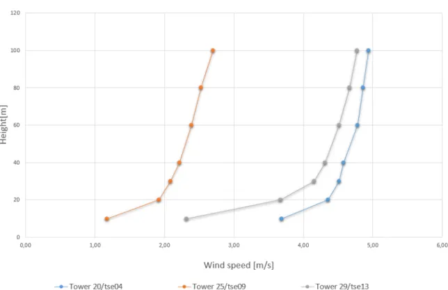
The data sets contained data from multiple towers and the first approach was to study the wind speed of the 100 meter towers (tower 20/tse04,tower 25/tse09 and tower 29/tse13) that had various 3D sonic anemometers at different heights (10 m, 20 m, 30 m, 40 m, 60 m, 80 m, 100 m) and their location is presented in figure2.3. Pandas was used to sort the data and create tables with the variables that were going to be analysed during the intensive observational period (IOP), which occurred between May 1st and June 15th of 2017.
Figure 2.3: Towers 20, 25 and 29 in serra do Perdigão.
In table 2.1 is presented the average wind speed of each day in the intensive observational period and max value registered by the sonic anemometers at 100 meters-high during each day. The tower that registered the maximum speed during this period was tower 29/tse13 located at second ridge of the valley and the top wind speed measured occurred on May 24 and its value was 17,71 m/s. Tower 20/tse04 that was located in the first ridge had a maximum wind speed measured of 13,95 m/s and it happened on May 11.
In figure 2.4 is presented the average wind speed along the towers with sonic anemometers with 100 m.
8 Methodology Table 2.1: Wind speed at 100 m towers
Tower 25/tse09 Tower 20/tse04 Tower 29/tse13 Day Mean Max Mean Max Mean Max 01/05/2017 3,11 4,14 3,11 5,83 3,23 6,51 02/05/2017 1,44 3,38 2,45 7,59 2,38 6,80 03/05/2017 2,95 5,39 4,92 9,03 4,50 8,29 04/05/2017 3,07 8,04 4,85 10,42 4,60 10,18 05/05/2017 3,90 8,17 7,71 12,72 7,22 11,96 06/05/2017 1,83 3,76 3,70 8,22 3,25 6,04 07/05/2017 2,82 6,11 5,27 9,10 4,73 8,39 08/05/2017 1,86 4,99 3,01 6,04 2,94 5,48 09/05/2017 2,50 5,05 6,00 11,99 5,38 9,76 10/05/2017 3,62 7,95 7,17 12,96 6,79 12,19 11/05/2017 4,48 8,38 9,57 13,95 8,91 12,70 12/05/2017 4,55 9,32 7,11 11,62 7,85 14,22 13/05/2017 2,25 5,94 5,15 9,81 5,17 10,43 14/05/2017 1,70 3,82 2,80 4,63 2,62 4,53 15/05/2017 2,14 5,26 4,10 7,83 3,69 7,05 16/05/2017 2,27 4,12 4,54 9,51 4,37 8,22 17/05/2017 2,72 8,92 4,36 9,88 4,16 8,65 18/05/2017 5,97 10,10 5,64 11,13 7,15 12,58 19/05/2017 2,60 5,16 6,25 12,01 5,50 9,43 20/05/2017 2,20 4,99 8,89 13,93 7,39 10,71 21/05/2017 4,21 8,15 8,93 16,34 7,75 12,58 22/05/2017 2,09 4,96 3,77 6,95 3,89 8,67 23/05/2017 2,01 5,00 7,88 12,24 6,64 9,49 24/05/2017 2,68 8,13 6,03 12,20 6,02 17,71 25/05/2017 1,56 3,34 2,39 6,14 4,59 14,76 26/05/2017 3,55 7,36 5,60 8,15 5,27 9,00 27/05/2017 2,13 5,83 3,91 6,86 3,86 7,91 28/05/2017 3,13 5,90 5,56 9,14 5,30 9,41 29/05/2017 2,08 6,85 3,45 7,94 3,29 7,07 30/05/2017 2,10 6,79 3,43 7,70 3,33 7,16 31/05/2017 2,11 8,15 4,27 9,53 3,92 8,40 01/06/2017 2,31 7,24 4,84 8,63 4,36 8,64 02/06/2017 2,58 7,91 4,14 10,04 3,80 9,48 03/06/2017 2,31 7,43 3,73 9,89 3,53 8,34 04/06/2017 4,09 9,74 4,50 11,58 5,57 13,01 05/06/2017 3,77 8,10 6,09 10,44 5,77 9,91 06/06/2017 3,37 6,89 4,26 7,10 4,83 7,70 07/06/2017 1,92 4,40 5,52 10,21 4,97 8,25 08/06/2017 2,70 7,84 5,32 9,49 5,04 10,28 09/06/2017 2,54 7,13 3,72 8,51 3,76 8,76 10/06/2017 1,89 5,83 3,96 7,45 3,72 6,79 11/06/2017 2,11 6,53 2,85 7,86 2,87 7,67 12/06/2017 2,15 6,67 4,59 8,62 4,29 7,87 13/06/2017 2,22 4,88 4,20 10,79 4,08 9,25 14/06/2017 2,46 6,43 4,56 8,06 4,54 8,49 15/06/2017 1,96 7,08 3,08 8,53 2,91 9,32
2.3 60 m towers 9
Figure 2.4: Wind speed averages variation with height during IOP.
2.3
60 m towers
The towers of 60 meters had 3D sonic anemometers at different heights(10 m, 20 m, 30 m, 40 m and 60 m) and their location is presented in figure2.5. Towers 34 and 37 were located on the southern ridge while towers 7, 22 and 27 are on the valley and tower 10 is located on the uphill side of the northern ridge.
Table 2.2: Locations of the 60 m towers Table No. Code Easting Northing 7 tnw07 33587.18 5351.36 10 tnw10 33952.07 5628.1 22 tse06 33636.59 4487.36 27 tse11 34334.33 4973.22 34 rsw03 33569.86 4006.84 37 rsw06 33087.97 4686.07
10 Methodology
Figure 2.5: Locations of the 60 m towers.
2.4
30 m towers
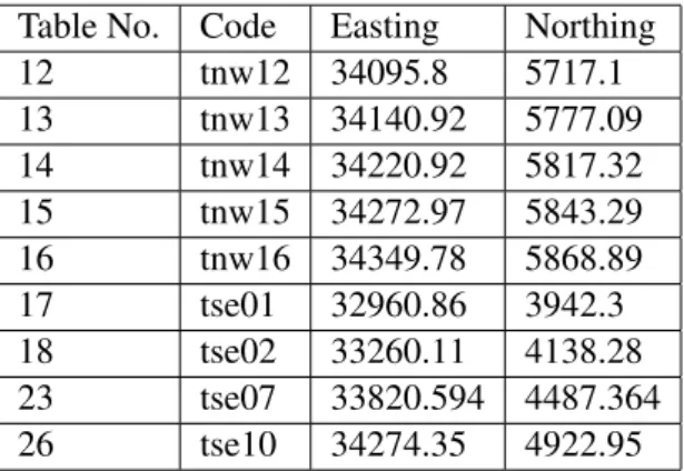
The towers of 30 meters had 3D sonic anemometers placed at different heights (2 m, 4 m, 6 m, 8 m, 10 m, 12 m, 20 m and 30 m) and their location is presented in figure2.6. Towers 12 through 16 are located on the side of the second ridge of the valley while towers 17, 18 are located on the first ridge and towers 23 and 26 are located in the valley between the ridges.
Table 2.3: Locations of the 30 m towers Table No. Code Easting Northing 12 tnw12 34095.8 5717.1 13 tnw13 34140.92 5777.09 14 tnw14 34220.92 5817.32 15 tnw15 34272.97 5843.29 16 tnw16 34349.78 5868.89 17 tse01 32960.86 3942.3 18 tse02 33260.11 4138.28 23 tse07 33820.594 4487.364 26 tse10 34274.35 4922.95
2.4 30 m towers 11
12 Methodology
2.5
20 m towers
The towers of 20 meters had 3D sonic anemometers at different heights(2 m, 4 m, 6 m, 8 m, 10 m,12 m and 20 m) and their location is presented in figure2.7. Tower 46, 11, 45 and 41 are located on top of the northern ridge while towers 39, 38, 33 and 32 are located in the southern ridge. Towers 1 and 2 are located on the uphill side of the southern ridge while towers 8 and 9 are located near the northern ridge. The other towers are on the valley between the two hills.
2.6 10 m towers 13 Table 2.4: Locations of the 20 m towers
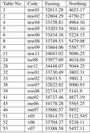
Table No. Code Easting Northing 1 tnw01 32611.28 4623.17 2 tnw02 32804.29 4750.27 4 tnw04 33158.81 4964.16 5 tnw05 33203.54 5041.16 6 tnw06 33434.16 5224.15 8 tnw08 33749.53 5479.08 9 tnw09 33864.06 5587.77 11 tnw11 34043.02 5696.25 24 tse08 33977.69 4634.04 28 tse12 34448.07 5044.25 32 rsw01 33730.49 3803.31 33 rsw02 33633.5 3901.2 38 rsw07 32822.82 5000.93 39 rsw08 32734.37 5141.9 41 rne02 34737.46 4877.19 45 rne06 34178.28 5565.25 46 rne07 33886.57 5852 51 v05 33814.75 5122.545 52 v06 33704.27 5238.11 53 v07 33388.58 5457.11
2.6
10 m towers
14 Methodology Table 2.5: Locations of the 10 m towers
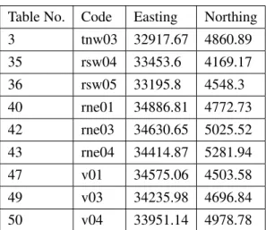
Table No. Code Easting Northing 3 tnw03 32917.67 4860.89 35 rsw04 33453.6 4169.17 36 rsw05 33195.8 4548.3 40 rne01 34886.81 4772.73 42 rne03 34630.65 5025.52 43 rne04 34414.87 5281.94 47 v01 34575.06 4503.58 49 v03 34235.98 4696.84 50 v04 33951.14 4978.78
2.7
Flow over Serra do Perdigão
The vast array of sensors and towers used on the Perdigão field experiment registered a large amount of variables associated with the flow and this work will focus on the flow parameters that concern with wind speed profile (u, v, w) and the turbulence kinetic energy.
The data obtained from the data sets was filtered by wind direction and divided in two groups: SW winds (225◦ ± 12.5◦) and NE winds (45◦ ± 12.5◦) to produce contour maps with the data
collected from the measurement campaign and make a comparison with flow simulation that was made before concerning this criteria. The contour maps include all the measurements made from the sonic anemometers of all the towers spread along the two ridges and in the valley that were equipped with them at the heights of 10, 20 and 30 meters.
To study the SW winds, the tower that was chosen as reference to filter the wind direction was tower no.16 (code tnw16) that was on the other side of the northern ridge before the wind flow started going uphill. The tower chosen to study the NE winds as tower no.20 (code tse04) that is located on the southern ridge. For the SW wind the wind direction was filtered at 30 meters a.g.l. and for NE winds the wind direction was filtered at 100 meters a.g.l..
After this filter was applied to the data variables, the data concerning the flow behaviour was appended and used to produce contour maps that show the towers layout in numbers and the values of each variable in a color gradient form. The contour maps were made for three different heights: 30, 20 and 10 meters a.g.l.. For 60 and 100 meters a.g.l. no contour maps were made because the maps for the 30 meters towers already presents a different and smaller shape because the number of towers is lower than the 20 meters and 10 meters towers. There are only 3 towers with 100 meters a.g.l. and only 9 towers with anemometers at 60 meters a.g.l.. The contour maps will be about the horizontal speed, the velocity components (u, v, w) and the Turbulent kinetic energy which depends of 3 variables (u_u, v_v and w_w).
Chapter 3
Results and discussion
In this chapter the results of the Serra do Perdigão campaign are presented and compared with the data from the flow simulation from (da Silva,2018). The results of the Serra do Perdigão are the measurements from the sonic anemometers that were assembled on the towers at 10, 20 and 30 meters (a.g.l.) are presented in sections3.1and3.2. First will be presented the results of this work and then will be made a comparison with the flow simulation and the flow patterns that were studied by (da Silva,2018) in section3.3.
3.1
Northeast winds
The Northeast winds (45◦) flow across the northern ridge (where are the towers in order along the ridge 46, 11, 45, 43, 29, 42, 41 and 40) over the valley to the southern ridge where are the towers from left to right 39, 38, 3, 37, 36, 20, 35, 34, 33 and 32), where it is possible to observe turbulence effects(e.g. detachment) when the flow reaches the top of both hills.
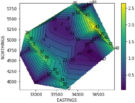
The flow from the NE winds shows that the speed is higher on the peak of the ridges and lower on the valley. The speed increases as the flow is climbing the ridges.
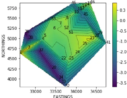
The stream-wise velocity component shows an inversion of direction(values change from posi-tive to negaposi-tive) after both ridges and in the middle of the valley. This is associated with turbulence more precisely due to the detachment of the flow on top of the hills and re-circulation of the flow in the middle of the valley.
For the NE winds the cross-stream component is positive in the direction of the tower no.32 to the tower no.39.
The cross-stream velocity component (v) values are predominantly positive for NE winds, the values positive or near zero after the northern ridge. The vertical velocity component (w) shows that the flow goes up both hills. The vertical component shows that the air flow goes up both ridges.
The turbulent kinetic energy for the NE winds presents higher values on the southern ridge where the flow accelerates.
18 Results and discussion
3.1.1 10 meters a.g.l.
The data from the towers of 10, 20, 30, 60 and 100 meters was used to plot the contour maps of the flow parameters that were the aim of the study (spd, u, v, w and TKE).The data that was used to make the maps is presented in appendixA.
3.1.1.1 Horizontal speed at 10 meters
3.1 Northeast winds 19 3.1.1.2 Velocity component u (stream-wise) at 10 meters a.g.l.
Figure 3.2: Velocity component u at 10 meters a.g.l (m/s)
3.1.1.3 Velocity component v (cross-stream) at 10 meters a.g.l.
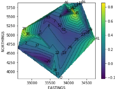
20 Results and discussion 3.1.1.4 Velocity component w (vertical) at 10 meters a.g.l.
Figure 3.4: Velocity component w at 10 meters a.g.l (m/s)
3.1.1.5 Turbulent kinetic energy at 10 meters a.g.l. [m2/s2]
3.1 Northeast winds 21
3.1.2 20 meters a.g.l.
The data from the towers of 20, 30, 60 and 100 meters was used to plot the contour maps of the flow parameters that were the aim of the study (spd, u, v, w and TKE).The data that was used to make the maps is presented in appendixA.
3.1.2.1 Horizontal speed 20 meters a.g.l.
22 Results and discussion 3.1.2.2 Velocity component u (stream-wise) at 20 meters a.g.l.
Figure 3.7: Horizontal speed at 20 meters a.g.l. (m/s)
3.1.2.3 Velocity component v (cross-stream) at 20 meters a.g.l.
3.1 Northeast winds 23 3.1.2.4 Velocity component w (vertical) at 20 meters a.g.l.
Figure 3.9: Velocity component w (vertical) at 20 meters a.g.l. (m/s)
3.1.2.5 Turbulent kinetic energy at 20 meters a.g.l. [m2/s2]
24 Results and discussion
3.1.3 30 meters a.g.l.
The data from the towers of 30, 60 and 100 meters was used to plot the contour maps of the flow parameters that were the aim of the study (spd, u, v, w and TKE). The data that was used to make the maps is presented in appendixA.
3.1.3.1 Horizontal speed 30 meters a.g.l.
3.1 Northeast winds 25 3.1.3.2 Velocity component u (stream-wise) at 30 meters a.g.l.
Figure 3.12: Velocity component u (stream-wise) at 30 meters a.g.l. (m/s)
3.1.3.3 Velocity component v (cross-stream) at 30 meters a.g.l.
26 Results and discussion 3.1.3.4 Velocity component w (vertical) at 30 meters a.g.l.
Figure 3.14: Velocity component v (stream-wise) at 30 meters a.g.l. (m/s)
3.1.3.5 Turbulent kinetic energy at 30 meters a.g.l. [m2/s2]
3.2 Southwest Winds 27
3.2
Southwest Winds
The Southwest winds (225◦) flow across the southern ridge over the valley to the northern ridge. On both ridges is possible to observe the detachment of the flow like it happens on the NE winds. The wind flow speed increases climbing both ridges and most part of the flow goes over the valley.
The stream-wise velocity component (u) shows an inversion of direction (values change from positive to negative) after the northern ridge and after the southern ridge in the region of towers number 1 and 2. After the peak of the northern ridge, the maps show detached flow on the valley and the re-circulation zone is noticeable in the valley dyed on purple on the stream-wise component contour maps of 10 meters.
The v values change to positive to negative with height. In the region of the valley the cross-stream component values are predominantly positive. When the flow approaches the southern ridge there is a inversion of direction the cross-stream component. It is also possible to see the effects of re-circulation of the flow in the valley region, the component is negative after the first ridge and in the middle of the valley starts to invert the direction.
The turbulence kinetic energy presented low values but it is as expected because this direction is one of the highest average velocity and lowest levels of turbulent intensity.
3.2.1 10 meters a.g.l.
The data from the towers of 10, 20, 30, 60 and 100 meters was used to plot the contour maps of the flow parameters that were the aim of the study (spd, u, v, w and TKE).The data that was used to make the maps is presented in appendixA.
28 Results and discussion 3.2.1.1 Horizontal wind speed at 10 meters a.g.l.
Figure 3.16: Horizontal speed at 10 meters a.g.l. (m/s)
3.2.1.2 Velocity component u (stream-wise) at 10 meters a.g.l.
3.2 Southwest Winds 29 3.2.1.3 Velocity component v (cross-stream) at 10 meters a.g.l.
Figure 3.18: Velocity component v (cross-stream) at 10 meters a.g.l. (m/s)
3.2.1.4 Velocity component w (vertical) at 10 meters a.g.l.
30 Results and discussion 3.2.1.5 Turbulent kinetic energy at 10 meters a.g.l. [m2/s2]
Figure 3.20: Turbulent kinetic energy at 10 meters a.g.l
3.2.2 20 meters a.g.l.
The data from the towers of 20, 30, 60 and 100 meters was used to plot the contour maps of the flow parameters that were the aim of the study (spd, u, v, w and TKE). The data that was used to make the maps is presented in appendixA.
3.2 Southwest Winds 31 3.2.2.1 Horizontal wind speed at 20 meters a.g.l.
Figure 3.21: Horizontal speed at 20 meters a.g.l. (m/s)
3.2.2.2 Velocity component u (stream-wise) at 20 meters a.g.l.
32 Results and discussion 3.2.2.3 Velocity component v (cross-stream) at 20 meters a.g.l.
Figure 3.23: Velocity component v (cross-stream) at 20 meters a.g.l. (m/s)
3.2.2.4 Velocity component w (vertical) at 20 meters a.g.l.
3.2 Southwest Winds 33 3.2.2.5 Turbulent kinetic energy at 20 meters a.g.l. [m2/s2]
Figure 3.25: Turbulent kinetic energy at 20 meters a.g.l.
3.2.3 30 meters a.g.l.
The data from the towers of 30, 60 and 100 meters was used to plot the contour maps of the flow parameters that were the aim of the study (spd, u, v, w and TKE). The data that was used to make the maps is presented in appendixA.
34 Results and discussion 3.2.3.1 Horizontal wind speed at 30 meters a.g.l.
Figure 3.26: Horizontal speed at 30 meters a.g.l. (m/s)
3.2.3.2 Velocity component u (stream-wise) at 30 meters a.g.l.
3.2 Southwest Winds 35 3.2.3.3 Velocity component v (cross-stream) at 30 meters a.g.l.
Figure 3.28: Velocity component v (cross-stream) at 30 meters a.g.l. (m/s)
3.2.3.4 Velocity component w (vertical) at 30 meters a.g.l.
36 Results and discussion 3.2.3.5 Turbulent kinetic energy at 30 meters a.g.l. [m2/s2]
Figure 3.30: Turbulent kinetic energy at 30 meters a.g.l
3.3
Comparison with flow simulation
On the two previous sections, the results of the measurements of the flow patterns made during the IOP of the Perdigão field experiment were presented and will be compared in this section with the flow simulation done by (da Silva,2018) concerning the two main wind directions Northeast (45◦) and Southwest (225◦).
3.3.1 Northeast winds
For the Northeast winds the simulation filtered the wind direction at 100 m a.g.l. at tower 20, with (45◦±15◦). The parameters of the wind flow measured have identical behaviour with the wind flow on the simulation over Perdigão.
The flow simulation shows that the cross-stream component (v) is predominantly positive on valley. It also shows an inversion of the direction with height. This variation with height was not observable in the contour maps for SW winds because the maximum height of the contour maps is only 30 meters a.g.l. and this variation occurs at 60 meters. This inversion was verified by the measurements of the sonic anemometers at 60 meters and 100 meters that displayed negative values for the v component on the northern ridge and the lee-side of the hill for SW winds. at 60 meters a.g.l. It was possible to see the inversion in the v component on the lee-side of the northern ridge with the data from the sonic anemometers at 60 meters a.g.l. of towers 29, 7 and 10. (appendixC)
3.3 Comparison with flow simulation 37
Figure 3.31: Flow simulation for NE winds for tower 20. (da Silva,2018)
For the NE winds, the flow simulation from (da Silva, 2018) studied 4 points for different surface cover models and that 4 points corresponded to the locations of the towers 37, 20, 25 and 29. The turbulent kinetic energy from the simulation displays the same variation from the data gathered through the Perdigão field experiment.
38 Results and discussion
Figure 3.33: Flow simulation for NE winds for tower 29. (da Silva,2018)
Figure 3.34: Flow simulation for NE winds for tower 25. (da Silva,2018)
The TKE values of the simulation for the NE winds are in accordance with the values that were observed on the measurements of Perdigão field experiment.
3.3 Comparison with flow simulation 39
3.3.2 Southwest winds
For the Southwest winds the simulation filtered the wind direction at 100m a.g.l. at tower 20, with (225◦± 15◦). In this work it was used the tower 16 at 30 meters located at the uphill side of the southern ridge for SW winds and used the same criteria for the wind direction(225◦± 15◦).
The simulation shows like in the data filtered from the field experiment the inversion of direc-tion in the wind profile in the valley due to re-circuladirec-tion of the detached flow for SW winds (the dashed line in figure3.35is where u = 0)
The flow simulation shows there is a inversion in the wind profile (the dashed line in3.35is where u=0), the v component changes from positive to negative with height. The same variation was observed on the contour maps that were plotted using the data of the measurements done and filtered by the wind direction.
Figure 3.35: Flow simulation for SW winds for tower 20. (da Silva,2018)
Concerning the turbulent kinetic energy, (da Silva,2018) studied 4 points, i.e, 4 towers (37, 20, 25 and 29).
The flow simulations from (da Silva,2018) display the same behaviour than the measurements, in this case, the turbulent kinetic energy of towers along the southern ridge (20 and 37). The turbulent kinetic energy for SW winds from the flow simulations done by (da Silva, 2018) is presented in figures3.36,3.37,3.38,3.39.
40 Results and discussion
Figure 3.36: Flow simulation for SW winds for tower 37. (da Silva,2018)
3.3 Comparison with flow simulation 41
Figure 3.38: Flow simulation for SW winds for tower 29. (da Silva,2018)
Figure 3.39: Flow simulation for SW winds for tower 25. (da Silva,2018)
The TKE values of the simulation for the SW winds are in accordance with the values that were observed on the measurements of Perdigão field experiment.
Chapter 4
Conclusions and future work
4.1
Conclusions
• The study of only one tower by itself is not enough to give a broad view of the environment surrounding it. For instance, a tower is unable to record data for high altitudes.
• The wind speed increases with height above ground level based on the data collected from the towers.
• After reviewing the towers data it can be seen that the prevailing wind direction is the one expected, NE and WSW, as observed previous measurements on the site.
• The average wind speed is also in accordance with previous measurements.
• The re-circulation in the valley, with its lower wind speeds and direction parallel to the ridges, could also be observed.
• As expected both wind directions presented low values of turbulence kinetic energy. In sections4.2and4.3will be presented the conclusion about the two groups of wind direction and the flow parameters.
4.2
Northeast winds
• Part of the flow goes above the double ridge, over the valley. The flow that fills valley area comes mostly from the gap on the south, corroborated by the cross-stream velocity component that is predominantly positive.
• The cross-stream velocity shows negative values at a higher height than the height used for the contour maps, at 60 meters a.g.l. it is possible to see the inversion in the v component on the lee-side of the northern ridge with the data from the sonic anemometers at 60 meters a.g.l. of towers 29, 7 and 10 .
44 Conclusions and future work • Flow detachment occurs right after reaching the peak of the northern ridge, and reattachment
occurs mainly when reaching the southern ridge.
• The turbulent kinetic energy for the NE winds are in accordance with the flow simulation
4.3
Southwest winds
• The flow in the central area of the southern ridge goes over the valley
• The stream-wise component inverts direction after the ridges where are the occurrences of flow separation on lee sides of hills (i.e. re-circulation zone) confirming the flow detachment occurs at both peaks.
• The cross-stream component shows and inversion of direction in the valley which means that flow started from going down to going up the valley.
• The data from the flow simulation using different surface cover models is in good corre-spondence with measurements for all variables.
• The turbulent kinetic energy for SW winds are in accordance with the flow simulation.
4.4
Future work
In order to improve the study of this object a few suggestions are presented:
• The data sets could be improved, they could be rearranged in ways to be more easier to sort through the data by defining some type of convention for all the data sets.
• Python scripts could be optimized for searching the data frames and getting all the data in a more effective way than collecting data one tower at a time.
• Compare the results of the measurements data with another experiences that are in the NEWA project in order to find correlations
• Select other towers as reference for the wind direction filter and compare them with the flow simulation
References
Carlos Alberto Madureira da Silva. Computational study of atmospheric flows over perdigao: Terrain resolution and domain size. July 2018. URL https://repositorio-aberto. up.pt/handle/10216/113854.
H. J. S. Fernando, J. Mann, J. M. L. M. Palma, J. K. Lundquist, R. J. Barthelmie, M. Belo-Pereira, W. O. J. Brown, F. K. Chow, T. Gerz, C. M. Hocut, P. M. Klein, L. S. Leo, J. C. Matos, S. P. Oncley, S. C. Pryor, L. Bariteau, T. M. Bell, N. Bodini, M. B. Carney, M. S. Courtney, E. D. Creegan, R. Dimitrova, S. Gomes, M. Hagen, J. O. Hyde, S. Kigle, R. Krishnamurthy, J. C. Lopes, L. Mazzaro, J. M. T. Neher, R. Menke, P. Murphy, L. Oswald, S. Otarola-Bustos, A. K. Pattantyus, C. Veiga Rodrigues, A. Schady, N. Sirin, S. Spuler, E. Svensson, J. Tomaszewski, D. D. Turner, L. van Veen, N. Vasiljevi´c, D. Vassallo, S. Voss, N. Wildmann, and Y. Wang. The Perdigão: Peering into microscale details of mountain winds. Bulletin of the American Meteorological Society, 100(5):799–819, 2019. URLhttps://journals.ametsoc.org/ doi/full/10.1175/BAMS-D-17-0227.1.
J.C. Kaimal and J.J. Finnigan. Atmospheric Boundary Layer Flows: Their Structure and Mea-surement. Oxford University Press, 1994. ISBN 9780195362770. URL https://books. google.pt/books?id=ljbSonRztIcC.
J. Mann, N. Angelou, J. Arnqvist, D. Callies, R. Chavez Arroyo E. Cantero, M. Courtney, J. Cuxart, E. Dellwik, J. Gottschall, S. Ivanell, P. Kuhn, G. Lea, J. C. Matos, J. M. L. M. Palma, L. Pauscher, A. Pena, J. Sanz Rodrigo, S. Soderberg, N. Vasiljevic, and C. Veiga Rodrigues. Complex terrain experiments in the new european wind atlas. The Royal Society Publishing, March 2017. URL https://royalsocietypublishing.org/doi/10.1098/rsta. 2016.0101.
N. Vasiljevic, J. M. L. M. Palma, N. Angelou, J. Carlos Matos, R. Menke, G. Lea, J. Mann, M. Courtney, L. Frolen Ribeiro, and V. M. M. G. C. Gomes. Perdigão 2015: methodology for atmospheric multi-doppler lidar experiments. Atmos. Meas. Tech., 10, 3463–3483, September 2017. URLhttps://doi.org/10.5194/amt-10-3463-2017.
Appendix A
Contour maps data
In this appendix are presented the tables containing all the data measured and used to plot the contour maps from the sonic anemometers filtered by wind direction, more precisely, southwest and northeast.
48 Contour maps data Table A.1: Horizontal speed at 10 meters a.g.l.
Tower NE SW 1 0.996079385 0.885568738 2 0.678350449 0.719130814 3 4.339088917 3.406280041 4 1.439563751 1.279410601 5 1.002253175 1.171657324 6 1.353189945 0.945774019 7 1.164724112 0.817538857 8 1.075739384 1.116333365 9 1.185899496 1.291831493 10 1.049432635 1.634035587 11 3.368149996 3.220199823 12 2.496266365 1.832148671 13 0.535334766 0.488034904 14 0.452274263 0.762800455 15 0.832481563 0.77483803 16 0.768665731 0.898026586 17 0.797507942 0.759653151 18 0.618471861 0.53607595 20 3.633528471 2.920635939 22 1.771085143 1.937520266 23 0.781847358 0.804183304 24 1.032391071 0.806460619 25 0.771425366 0.720478296 26 0.460380971 0.480990171 27 0.672282279 0.814115226 28 0.33247003 0.454356521 29 1.314827561 2.546877146 32 3.521439552 2.628167868 33 1.564546466 2.628167868 34 4.327646255 3.084823608 35 4.060050011 3.163723707 36 4.764554501 3.338205814 37 4.689229965 3.376245022 38 4.570497513 3.270372391 39 4.939497948 3.409882784 40 2.408607244 2.985109806 41 1.247911572 2.941128492 42 3.451375484 3.521998405 43 3.229536772 3.81268692 45 3.531733513 3.33993268 46 4.247181416 3.390903711 47 0.653919578 0.561717749 49 0.798556328 0.676091433 50 1.206554413 1.00358212 51 0.771873653 0.552566409 52 1.245778203 0.885558546 53 1.171598554 0.815716147
Contour maps data 49 Table A.2: Velocity component u (stream-wise) at 10 meters a.g.l.
Tower NE SW 1 0.150420263 -0.340571761 2 0.06329944 -0.028432706 3 -3.057132244 1.410051703 4 -0.53949672 0.158920228 5 -0.202070683 0.210451439 6 -0.436494976 -0.169613689 7 -0.285929471 -0.310783446 8 -0.20746249 -0.216732517 9 -0.252171397 0.26269269 10 -0.20908314 0.71180445 11 -1.853096962 1.606750846 12 -1.36851716 1.013262153 13 -0.299815267 0.116855495 14 0.02043869 0.364117742 15 -0.234583795 0.408508003 16 -0.187935516 0.458957791 17 0.044731829 -0.276897997 18 -0.049683377 0.020409578 20 -2.759637833 1.719873548 22 -0.836997747 0.735282421 23 -0.163184732 0.090348922 24 -0.143865034 -0.074746266 25 -0.103918768 -0.256594568 26 0.154514 0.074306749 27 0.004697094 -0.076802053 28 -0.070866175 0.116010159 29 -0.685929418 1.341935992 32 -2.005793095 1.259453177 33 -0.936357319 1.256311417 34 -3.250297308 1.601078272 35 -2.808400869 1.65656507 36 -3.395168781 1.439294219 37 -3.15209794 1.421987414 38 -3.321108341 1.300378084 39 -3.748301506 1.220072389 40 -1.06484437 1.28191185 41 -0.61283952 1.489151597 42 -2.263475895 1.68319118 43 -1.996652722 1.927700281 45 -2.182682276 1.613070369 46 -1.968460083 1.892491102 47 -0.059953358 -0.063376419 49 -0.11082717 -0.235583887 50 -0.290457249 -0.458955556 51 -0.058938053 -0.131049827 52 -0.264447004 -0.393738329 53 -0.343198299 -0.40638715
50 Contour maps data Table A.3: Velocity component v (cross-stream) at 10 meters a.g.l.
Tower SW NE 1 0.047682438 0.278520316 2 0.084385887 0.35054183 3 -2.639026642 2.149255753 4 -0.675236404 0.621404767 5 -0.221259892 0.677042067 6 -0.057167463 0.283163369 7 0.519622445 0.230972588 8 0.257494867 0.359300971 9 0.08387588 0.736850083 10 0.076008514 1.034232616 11 -2.352679253 2.20851326 12 -1.58190763 0.950784266 13 -0.181089208 0.067460708 14 -0.084175751 0.338553339 15 -0.189192921 0.335010558 16 -0.137983456 0.430335253 17 -0.036248643 0.076938622 18 -0.008753137 0.19463326 20 -1.851924181 1.433454037 22 -1.0729177 1.100434542 23 -0.319248497 0.301489025 24 -0.167344362 0.295839459 25 0.28242892 0.298577607 26 0.091275513 0.164094627 27 0.116068505 0.382360756 28 0.045145966 0.166021258 29 -0.726971209 1.640000701 32 -2.582092285 1.441856861 33 -0.802635014 1.779100418 34 -2.420182467 1.619004965 35 -2.523178816 1.69574964 36 -2.900910854 2.006199598 37 -3.044937611 2.074038506 38 -2.630656958 1.826919436 39 -2.615608692 2.188546419 40 -1.807565331 2.019871712 41 -0.739454508 1.908146143 42 -2.132264614 2.23188448 43 -1.94501245 2.637950659 45 -2.294024944 2.218443394 46 -3.360541582 1.862842441 47 0.192844912 0.139824599 49 0.135774389 0.058140732 50 0.525507629 0.43558079 51 0.291523129 0.220349595 52 0.484134644 0.278048754 53 0.545414746 0.226165056
Contour maps data 51 Table A.4: Velocity component w (vertical) at 10 meters a.g.l.
Tower NE SW 1 -0.004884748 -0.058759805 2 0.025940917 0.117712379 3 0.352408826 0.342600763 4 0.183450326 -0.261731803 5 -0.005243114 -0.207298651 6 0.019346289 -0.053819913 7 -0.034534592 -0.025244169 8 0.065987915 0.085673988 9 -0.013240212 0.220063418 10 -0.090339474 0.351472706 11 0.257337302 0.016133791 12 0.82119 -0.522446334 13 0.124609515 -0.06092111 14 0.020830216 -0.236754209 15 0.008557542 -0.164988816 16 0.015749773 -0.142158285 17 -0.015429433 -0.061507683 18 -0.017833829 0.044386636 20 -0.348102063 0.404911518 22 0.157823116 -0.206413344 23 -0.015173856 -0.10718184 24 -0.034905311 -0.061640088 25 -0.002058488 -0.01359445 26 0.082544081 0.057443354 27 0.003882872 0.018586051 28 0.014655886 0.062377587 29 -0.040654074 0.107647054 32 0.082392618 0.155218601 33 0.084535956 0.335475802 34 0.227482796 0.036918867 35 0.114535958 0.247285262 36 -0.087057419 0.064365022 37 0.322110742 0.201839745 38 0.592773974 0.136557594 39 0.853552938 0.154294774 40 0.047416005 -0.04018477 41 0.148051888 0.311380595 42 0.510737598 0.02432055 43 0.90574342 0.119739428 45 0.620276213 -0.08762195 46 0.501090705 -0.188442498 47 -0.001874474 0.008003634 49 -0.016178874 0.013672399 50 -0.030869871 -0.024110574 51 -0.022320293 0.003630128 52 4.47E-05 0.00859783 53 -0.044714201 -0.041674595
52 Contour maps data Table A.5: Turbulent kinetic energy at 10 meters-high anemometers
Tower NE SW 1 0.180476 0.039899 2 0.050957 0.032405 3 0.594495 0.071503 4 0.358368 0.161187 5 0.1584 0.118266 6 0.396928 0.080981 7 0.1343 0.036434 8 0.13872 0.080246 9 0.178762 0.092146 10 0.136799 0.099668 11 0.156798 0.138859 12 0.173515 0.203834 13 0.012423 0.028375 14 0.006191 0.108358 15 0.047592 0.095595 16 0.044486 0.147942 17 0.101723 0.02294 18 0.035239 0.012539 20 0.510841 0.093982 22 0.323325 0.282755 23 0.081916 0.084846 24 0.185589 0.055515 25 0.035604 0.021889 26 0.015143 0.016786 27 0.047664 0.054763 28 0.00435 0.003345 29 0.113613 0.157245 32 0.973922 0.097461 33 0.597753 0.070872 34 0.43437 0.089289 35 0.856242 0.106318 36 0.52766 0.08905 37 0.538768 0.069837 38 0.939955 0.142054 39 0.927454 0.072987 40 0.190236 0.159964 41 0.078847 0.140801 42 0.177145 0.123811 43 0.108254 0.123712 45 0.136198 0.175152 46 0.154329 0.151304 47 0.028017 0.01365 49 0.069449 0.02163 50 0.107955 0.048337 51 0.061206 0.01763 52 0.13744 0.037319 53 0.144124 0.030107
Contour maps data 53
Table A.6: Horizontal speed at 20 meters a.g.l. Tower NE SW 1 1.317096 1.243178 2 0.977508 1.402474 4 1.825462 1.932096 5 1.361202 1.814814 6 1.431888 1.160006 7 1.621153 1.210131 8 1.217625 1.281129 10 1.612878 1.999774 11 3.808395 3.199825 12 3.025759 3.212981 13 1.68192 1.865587 14 1.306366 2.003959 15 1.249498 2.16093 16 1.140229 2.168176 20 4.935785 3.242028 22 1.989916 2.225099 23 1.221136 1.309147 24 1.409168 1.300087 25 1.248299 1.280383 27 0.960568 1.28778 28 0.976271 1.827036 29 3.516235 3.246995 32 4.555236 3.238486 33 4.76594 3.492126 34 4.797439 3.479818 37 5.052225 3.454655 38 4.920872 3.571425 39 4.979286 3.421537 41 3.743184 3.416035 45 3.861491 3.625047 46 4.524894 3.453052 51 1.533492 1.218332 52 1.516318 1.161791 53 1.534725 1.090791
54 Contour maps data
Table A.7: Velocity component u (stream-wise) at 20 meters a.g.l. Tower NE SW 1 0.337226 -0.30015 2 0.295839 0.079385 4 -0.84158 0.433115 5 -0.48485 0.420834 6 -0.54774 -0.17012 7 -0.58821 -0.50787 8 -0.23092 -0.12027 10 -0.6303 0.722606 11 -2.18417 1.614161 12 -1.68963 1.87217 13 -0.64188 0.913414 14 -0.3759 1.141099 15 -0.27658 1.284582 16 -0.22327 1.389964 20 -3.45021 1.581467 22 -1.02637 0.917897 23 -0.4665 0.263032 24 -0.32593 0.005182 25 -0.17623 -0.46774 27 0.073282 -0.13287 28 -0.08413 0.360752 29 -2.05532 1.529572 32 -2.62764 1.183586 33 -3.19034 1.273736 34 -3.40265 1.639927 37 -3.31183 1.385378 38 -3.41483 1.456756 39 -3.69367 1.274777 41 -1.74186 1.524906 45 -2.26351 1.661421 46 -2.22713 1.963678 51 -0.42223 -0.52378 52 -0.41147 -0.50574 53 -0.61431 -0.50313
Contour maps data 55
Table A.8: Velocity component v (cross-stream) at 20 meters a.g.l. Tower SW NE 1 0.140452 0.727562 2 0.244848 0.976109 4 -0.90977 1.178614 5 -0.47345 1.120423 6 -0.15446 0.370821 7 0.722175 0.456009 8 0.289925 0.537841 10 -0.41281 1.353646 11 -2.568 1.893139 12 -1.9511 2.019561 13 -0.93889 1.012044 14 -0.66446 1.214592 15 -0.54925 1.408605 16 -0.40663 1.381611 20 -3.13075 1.724271 22 -1.21431 1.284104 23 -0.6108 0.706808 24 -0.53339 0.606854 25 0.482571 0.600533 27 0.246182 0.780442 28 0.110057 1.270733 29 -2.41316 1.957927 32 -3.37374 1.972158 33 -3.11342 1.944519 34 -2.97404 1.925948 37 -3.39417 2.067497 38 -3.08717 2.145778 39 -2.81826 2.06886 41 -2.95287 2.025533 45 -2.64671 2.446574 46 -3.54647 1.768544 51 0.573292 0.511506 52 0.662214 0.508783 53 0.714307 0.382522
56 Contour maps data
Table A.9: Velocity component w (vertical) at 20 meters a.g.l. Tower NE SW 1 0.046169 0.032795 2 0.160685 0.226242 4 0.352085 -0.35215 5 0.066858 -0.28171 6 0.083391 -0.02885 7 -0.04172 -0.03513 8 0.076949 0.129134 10 -0.21759 0.382656 11 0.532091 -0.13378 12 0.855415 -0.78366 13 0.351082 -0.59462 14 0.207303 -0.71852 15 0.135765 -0.66622 16 0.099175 -0.56037 20 -0.18025 0.368415 22 0.199088 -0.2467 23 0.068319 -0.13 24 0.062338 0.00044 25 0.041631 0.017091 27 0.035618 0.064633 28 -0.01352 0.356277 29 0.041726 0.184558 32 0.218471 0.170432 33 0.265979 0.352696 34 0.312466 0.039631 37 0.179901 0.204613 38 0.717942 0.142082 39 0.765049 0.038815 41 0.602479 0.19535 45 0.752877 -0.2155 46 0.415877 -0.12786 51 -0.01551 0.013266 52 -0.03088 -0.01564 53 -0.04483 -0.03685
Contour maps data 57
Table A.10: Turbulent kinetic energy at 20 meters-high anemometers Tower NE SW 1 0.268322 0.054721 2 0.123916 0.063817 4 0.475262 0.243518 5 0.323028 0.237359 6 0.38581 0.112318 7 0.197789 0.056505 8 0.189442 0.096825 10 0.34871 0.113269 11 0.131714 0.104007 12 0.142319 0.186071 13 0.112855 0.408709 14 0.100761 0.545687 15 0.085761 0.5786 16 0.081034 0.505233 20 0.417417 0.072691 22 0.357115 0.294775 23 0.238526 0.17233 24 0.33648 0.152687 25 0.144969 0.069283 27 0.100629 0.101723 28 0.102021 0.129144 29 0.183647 0.117355 32 0.435931 0.07262 33 0.866184 0.110735 34 0.318224 0.066171 37 0.427238 0.062775 38 0.707003 0.064998 39 0.711187 0.061004 41 0.120397 0.123472 45 0.103969 0.139326 46 0.128222 0.122433 51 0.189217 0.064652 52 0.172806 0.052444 53 0.210743 0.048299
58 Contour maps data
Table A.11: Horizontal speed at 30 meters a.g.l. Tower NE SW 7 1.668735 1.309707 10 2.261665 2.179466 12 3.288405 3.484736 13 2.021331 2.347137 14 1.616657 2.484787 15 1.574639 2.812908 16 1.31971 2.53803 17 1.231425 1.217473 18 1.224714 1.394044 20 5.144668 3.29831 22 2.178338 2.458524 25 1.278869 1.385996 26 1.155875 1.39145 27 1.154173 1.585468 29 4.11641 3.387784 34 4.981642 3.473818 37 5.195449 3.465762
Table A.12: Velocity component u (stream-wise) at 30 meters a.g.l. Tower NE SW 7 -0.61494 -0.50454 10 -1.14818 0.78887 12 -1.91781 1.953106 13 -0.91619 1.331459 14 -0.53675 1.428183 15 -0.3817 1.596535 16 -0.30781 1.655995 17 0.14572 -0.10265 18 0.258104 0.229536 20 -3.58051 1.607319 22 -1.20631 1.097579 25 -0.11923 -0.40478 26 -0.02866 -0.33051 27 0.097996 -0.10449 29 -2.42652 1.696983 34 -3.45476 1.633107 37 -3.46106 1.456245
Contour maps data 59
Table A.13: Velocity component v (cross-stream) at 30 meters a.g.l. Tower SW NE 7 0.687802 0.514499 10 -1.13809 1.458086 12 -2.13109 2.227427 13 -1.10984 1.312637 14 -0.8602 1.57757 15 -0.81245 1.985312 16 -0.53619 1.677326 17 -0.20999 0.727737 18 -0.00924 0.990653 20 -3.31165 1.703269 22 -1.34485 1.424656 25 0.405127 0.707738 26 0.083041 0.653583 27 0.245282 1.042876 29 -2.89848 1.866165 34 -3.24176 1.836642 37 -3.50382 1.923009
Table A.14: Velocity component w (vertical) at 30 meters a.g.l. Tower NE SW 7 -0.05258 -0.04774 10 -0.34901 0.366694 12 0.825272 -0.73786 13 0.472033 -0.86949 14 0.273173 -0.82864 15 0.252556 -0.99533 16 0.133 -0.63249 17 -0.00133 0.028369 18 0.062705 0.203709 20 -0.1629 0.325127 22 0.226348 -0.29089 25 0.027269 0.012709 26 0.116561 0.116072 27 0.035211 0.095216 29 0.285372 0.018001 34 0.317286 0.031149 37 0.255771 0.094615
60 Contour maps data
Table A.15: Turbulent kinetic energy at 30 meters-high anemometers Tower NE SW 7 0.228232 0.068788 10 0.526663 0.117665 12 0.139453 0.150824 13 0.106435 0.5101 14 0.103858 0.530983 15 0.115942 0.669607 16 0.090109 0.506115 17 0.280163 0.050692 18 0.202832 0.064898 20 0.337031 0.064235 22 0.386976 0.277563 25 0.189188 0.077829 26 0.140592 0.103394 27 0.14594 0.114053 29 0.110833 0.11 34 0.287728 0.060623 37 0.401056 0.064088
Appendix B
Python scripts
In this appendix are presented some of the scripts used to read the NetCDF files, the change from data set to data frame and the concatenation of the files the IOP. An example of the scripts used for the contour maps is also shown, in this case, is shown the script for horizontal speed at 30 meters a.g.l. . After the files were all concatenated and merged into one file containing all the data for the IOP, there were applied some filters, more precisely, for the wind direction. For the SW winds the wind direction was filtered for 225±12.5 degrees and for the NE winds the wind direction was filtered for 45±12.5 degrees. The coordinates x and y in the contour map script represent the eastings and northings of each tower and the n variable represents, in the example presented in this section, the horizontal speed at 30 meters above ground level. These contour maps were made for the variables u, v, w, T.K.E and horizontal speed for 30, 20 and 10 meters a.g.l. .
62 Python scripts import xarray as xr ds1=xr.open_dataset(’E:/MEDICOES MAIO/isfs_qc_tiltcor_20170501.nc’) ds2=xr.open_dataset(’E:/MEDICOES MAIO/isfs_qc_tiltcor_20170502.nc’) ds3=xr.open_dataset(’E:/MEDICOES MAIO/isfs_qc_tiltcor_20170503.nc’) ds4=xr.open_dataset(’E:/MEDICOES MAIO/isfs_qc_tiltcor_20170504.nc’) ds5=xr.open_dataset(’E:/MEDICOES MAIO/isfs_qc_tiltcor_20170505.nc’) ds6=xr.open_dataset(’E:/MEDICOES MAIO/isfs_qc_tiltcor_20170506.nc’) ds7=xr.open_dataset(’E:/MEDICOES MAIO/isfs_qc_tiltcor_20170507.nc’) ds8=xr.open_dataset(’E:/MEDICOES MAIO/isfs_qc_tiltcor_20170508.nc’) ds9=xr.open_dataset(’E:/MEDICOES MAIO/isfs_qc_tiltcor_20170509.nc’) ds10=xr.open_dataset(’E:/MEDICOES MAIO/isfs_qc_tiltcor_20170510.nc’) ds11=xr.open_dataset(’E:/MEDICOES MAIO/isfs_qc_tiltcor_20170511.nc’) ds12=xr.open_dataset(’E:/MEDICOES MAIO/isfs_qc_tiltcor_20170512.nc’) ds13=xr.open_dataset(’E:/MEDICOES MAIO/isfs_qc_tiltcor_20170513.nc’) ds14=xr.open_dataset(’E:/MEDICOES MAIO/isfs_qc_tiltcor_20170514.nc’) ds15=xr.open_dataset(’E:/MEDICOES MAIO/isfs_qc_tiltcor_20170515.nc’) ds16=xr.open_dataset(’E:/MEDICOES MAIO/isfs_qc_tiltcor_20170516.nc’) ds17=xr.open_dataset(’E:/MEDICOES MAIO/isfs_qc_tiltcor_20170517.nc’) ds18=xr.open_dataset(’E:/MEDICOES MAIO/isfs_qc_tiltcor_20170518.nc’) ds19=xr.open_dataset(’E:/MEDICOES MAIO/isfs_qc_tiltcor_20170519.nc’) ds20=xr.open_dataset(’E:/MEDICOES MAIO/isfs_qc_tiltcor_20170520.nc’) ds21=xr.open_dataset(’E:/MEDICOES MAIO/isfs_qc_tiltcor_20170521.nc’) ds22=xr.open_dataset(’E:/MEDICOES MAIO/isfs_qc_tiltcor_20170522.nc’) ds23=xr.open_dataset(’E:/MEDICOES MAIO/isfs_qc_tiltcor_20170523.nc’) ds24=xr.open_dataset(’E:/MEDICOES MAIO/isfs_qc_tiltcor_20170524.nc’) ds25=xr.open_dataset(’E:/MEDICOES MAIO/isfs_qc_tiltcor_20170525.nc’) ds26=xr.open_dataset(’E:/MEDICOES MAIO/isfs_qc_tiltcor_20170526.nc’) ds27=xr.open_dataset(’E:/MEDICOES MAIO/isfs_qc_tiltcor_20170527.nc’) ds28=xr.open_dataset(’E:/MEDICOES MAIO/isfs_qc_tiltcor_20170528.nc’) ds29=xr.open_dataset(’E:/MEDICOES MAIO/isfs_qc_tiltcor_20170529.nc’) ds30=xr.open_dataset(’E:/MEDICOES MAIO/isfs_qc_tiltcor_20170530.nc’) ds31=xr.open_dataset(’E:/MEDICOES MAIO/isfs_qc_tiltcor_20170531.nc’) ds32=xr.open_dataset(’E:/MEDICOES JUNHO/isfs_qc_tiltcor_20170601.nc’) ds33=xr.open_dataset(’E:/MEDICOES JUNHO/isfs_qc_tiltcor_20170602.nc’) ds34=xr.open_dataset(’E:/MEDICOES JUNHO/isfs_qc_tiltcor_20170603.nc’) ds35=xr.open_dataset(’E:/MEDICOES JUNHO/isfs_qc_tiltcor_20170604.nc’) ds36=xr.open_dataset(’E:/MEDICOES JUNHO/isfs_qc_tiltcor_20170605.nc’) ds37=xr.open_dataset(’E:/MEDICOES JUNHO/isfs_qc_tiltcor_20170606.nc’) ds38=xr.open_dataset(’E:/MEDICOES JUNHO/isfs_qc_tiltcor_20170607.nc’) ds39=xr.open_dataset(’E:/MEDICOES JUNHO/isfs_qc_tiltcor_20170608.nc’) ds40=xr.open_dataset(’E:/MEDICOES JUNHO/isfs_qc_tiltcor_20170609.nc’) ds41=xr.open_dataset(’E:/MEDICOES JUNHO/isfs_qc_tiltcor_20170610.nc’) ds42=xr.open_dataset(’E:/MEDICOES JUNHO/isfs_qc_tiltcor_20170611.nc’) ds43=xr.open_dataset(’E:/MEDICOES JUNHO/isfs_qc_tiltcor_20170612.nc’) ds44=xr.open_dataset(’E:/MEDICOES JUNHO/isfs_qc_tiltcor_20170613.nc’) ds45=xr.open_dataset(’E:/MEDICOES JUNHO/isfs_qc_tiltcor_20170614.nc’) ds46=xr.open_dataset(’E:/MEDICOES JUNHO/isfs_qc_tiltcor_20170615.nc’)
Python scripts 63 df1=ds1.to_dataframe() df2=ds2.to_dataframe() df3=ds3.to_dataframe() df4=ds4.to_dataframe() df5=ds5.to_dataframe() df6=ds6.to_dataframe() df7=ds7.to_dataframe() df8=ds8.to_dataframe() df9=ds9.to_dataframe() df10=ds10.to_dataframe() df11=ds11.to_dataframe() df12=ds12.to_dataframe() df13=ds13.to_dataframe() df14=ds14.to_dataframe() df15=ds15.to_dataframe() df16=ds16.to_dataframe() df17=ds17.to_dataframe() df18=ds18.to_dataframe() df19=ds19.to_dataframe() df20=ds20.to_dataframe() df21=ds21.to_dataframe() df22=ds22.to_dataframe() df23=ds23.to_dataframe() df24=ds24.to_dataframe() df25=ds25.to_dataframe() df26=ds26.to_dataframe() df27=ds27.to_dataframe() df28=ds28.to_dataframe() df29=ds29.to_dataframe() ... df46=ds46.to_dataframe() dfs=[df1,....,df46] for df in dfs: df.reset_index(inplace=True) import pandas as pd dados = pd.concat(dfs) NE filter
A=dados[(dados.dir_100m_tse04 >=32.5) & (dados.dir_100m_tse04<=57.5)] SW filter
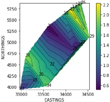
64 Python scripts import numpy as np import matplotlib.pyplot as plt import scipy.interpolate # torres 7,10,12,13,14,15,16,17,18,20,22,25,26,27,29,34,37 x = [33587.18,33952.07,34095.8,34140.92,34220.92,34272.97,34349.78,32960.86,33260.11,33394.18,33636.59,34153.02,34274.35,34334.33,34533.6,33569.86,33087.97] y = [5351.36,5628.1,5717.1,5777.09,5817.32,5843.29,5868.89,3942.3,4138.28,4258.87,4487.36,4844.78,4922.95,4973.22,5112.01,4006.84,4686.07] n = [1.66873467,2.261664867,3.288404703,2.02133131,1.616657495,1.574639082,1.319709778,1.231425166,1.224714041,5.144668102,2.178338051,1.278869033,1.15587461,1.154173017,4.116410255,4.981641769,5.195448875] # convert list of data to arrays
x = np.asarray(x) y = np.asarray(y) z = np.asarray(n)
# Set up a regular grid of interpolation points nInterp = 200
xi, yi = np.linspace(x.min(), x.max(), nInterp), np.linspace(y.min(), y.max(), nInterp) xi, yi = np.meshgrid(xi, yi)
# Interpolate; there’s also method=’cubic’ for 2-D data such as here #rbf = scipy.interpolate.Rbf(x, y, z, function=’linear’)
#zi = rbf(xi, yi)
zi = scipy.interpolate.griddata((x, y), z, (xi, yi), method=’linear’) #contour lines
CS = plt.contour(xi, yi, zi, 15, linewidths=0.5, colors=’k’) plt.imshow(zi, vmin=z.min(), vmax=z.max(), origin=’lower’, extent=[x.min(), x.max(), y.min(), y.max()])
plt.xlabel("EASTINGS") plt.ylabel("NORTHINGS") plt.text(33587.18,5351.36,’7’) plt.text(33952.07,5628.1,’10’) plt.text(34095.8,5717.1,’12’) plt.text(34140.92,5777.09,’13’) plt.text(34220.92,5817.32,’14’) plt.text(34272.97,5843.29,’15’) plt.text(34349.78,5868.89,’16’) plt.text(32960.86,3942.3,’17’) plt.text(33260.11,4138.28,’18’) plt.text(33394.18,4258.87,’20’) plt.text(33636.59,4487.36,’22’) plt.text(34153.02,4844.78,’25’) plt.text(34274.35,4922.95,’26’) plt.text(34334.33,4973.22,’27’) plt.text(34533.6,5112.01,’29’) plt.text(33569.86,4006.84,’34’) plt.text(33087.97,4686.07,’37’) plt.colorbar() plt.show()
Appendix C
Cross-stream (v) values for 60 meters
and 100 meters for NE winds
Here are presented v values for the NE winds (45 degrees)
Figure C.1: Tower 29 NE winds v component at 60 meters a.g.l.
66 Cross-stream (v) values for 60 meters and 100 meters for NE winds
Figure C.2: Tower 7 NE winds v component at 60 meters a.g.l.