3D Points Recover From Stereo Video Sequences
Based on
OpenCV 2.1 Libraries
A Thesis Presented to the Faculty of Mechanical Engineering and Robotics
AGH University of Science and Technology of Krakow
In Partial Fulfillment of the Requirements of the Degree of
Master of Science
in
Mechanical Engineering
by
Rosério D. V. Valente
July 22, 2011
3D Points Recover From Stereo Video Sequences
Based on
OpenCV 2.1 Libraries
In Partial Fulfillment of the Requirements of the Degree of
Master of Science
in
Mechanical Engineering
by Rosério D. V. Valente
Faculty of Mechanical Engineering and Robotics
AGH University of Science and Technology of Krakow
July 22, 2011
Under the guidance and approval of the committee, and approved by all its members, this thesis has been accepted in partial fulfillment of the requirements for the degree.
Approved:
Chairperson (Dr. Piotr Kohut) Date
1 Acknowledgements
It is a pleasure to thank those who made this thesis possible, supporting it directly and indirectly. First of all I would like to thank my supervisor, Dr. Piotr Kohut, for his guidance, advice and specially for his time during the numerous meetings and laboratory experiments that enabled me to achieve better results and a deeper understanding on the subject. Also, I would like to thank Dr. Wojciech Lisowski to whom I owe my deepest gratitude for his support and assistance since the start of my stage as erasmus student at AGH University and for his comprehension and kindness during all the process. I would like to thank my mum Gabriela and my sisters Mary and Fernanda for being always supportive even when I spend long time far from them. I would like to thank Paula Olim for her friendship, kindness and encouragement and to make me believe that it is always possible to go further. Also I would like to show my gratitude to Olinha for her support, joy and company and to all my friends who have been helping and supporting me on my goals and ambitions.
Lastly, but not the least, I would like to thank all the OpenCV community for providing a great support to all of those interested in learning OpenCV. Finally I would like also to tank all the authors who provided all the interesting research and literature on stereo vision.
2 Abstract
The purpose of this study was to implement a program in C++ using OpenCV image processing platform's algorithms and Microsoft Visual Studio 2008 development environment to perform cameras calibration and calibration parameters optimization, stereo rectification, stereo correspondence and recover sets of 3D points from a pair of synchronized video sequences obtained
from a stereo configuration. The study utilized two pretest laboratory sessions and one intervention laboratory session. Measurements included setting different stereo configurations with two Phantom v9.1 high-speed cameras to: capture video sequences of a MELFA RV-2AJ robot executing a
simple 3D path, and additionally capture video sequences of a planar calibration object, being
moved by a person, to calibrate each stereo configuration. Significant improvements were made from pretest to intervention laboratory session on minimizing procedures errors and choosing the best camera capture settings. Cameras intrinsic and extrinsic parameters, stereo relations, and disparity-to-depth matrix were better estimated for the last measurements and the comparison between the obtained sets of 3D points (3D path) with the robot's 3D path proved to be similar.
RECOVERING 3D POINTS FROM STEREO VIDEO SEQUENCES
BASED ON OPEN CV 2.1 LIBRARIES
1Acknowledgements...iii 2Abstract...iv 3Index of Tables...vii 4Illustration Index...viii 5Chapter One...1 5.1Introduction...1
5.1.1Statement of the Problem...2
5.1.2Background and Need...3
5.1.3Purpose of the Study...5
5.1.4Research Questions...6
5.1.5Significance of the field...6
5.1.6Definitions...7
5.1.7Limitations...9
6Chapter Two...10
6.1Review of the Literature...10
6.1.1Introduction...10 6.1.2Research Synthesis...10 6.1.3Summary...36 7Chapter Three...37 7.1Methods...37 7.1.1Introduction...37 7.1.2Settings...38
7.1.3Intervention and Instructional Materials...38
7.1.4Measurements Instruments...39
7.1.5Procedures...41
8Chapter Four ...63
8.1Results...63
8.1.1Introduction ...63
8.1.2Research Question Nº1 – Results...68
8.1.3Research Question Nº2 – Results...68
8.1.4Research Question Nº3 – Results...81
8.1.5Research Question Nº4 – Results...82
8.1.6Research Question Nº5 – Results...84
9Chapter Five...88
9.1Discussion ...88
9.1.1Introduction...88
9.1.2Discussion ...88
9.1.3Limitations...93
9.1.4Recommendations for Future Research ...94
9.1.5Conclusions...94
10References...96
11Appendix A: Stereo Imaging...99
11.1Stereo Imaging...100
11.1.1Introduction...100
11.1.2Working With a Single Camera...100
11.1.4Camera Calibration ...106
11.1.5Undistortion...108
11.2Working With Two Cameras ...111
11.2.1Stereo Imaging ...111
11.2.2 Stereo Calibration...114
11.2.3Stereo Rectification...115
11.2.4Stereo Correspondence...117
12Appendix B: MELFA Basic IV Presentation...120
13Appendix C: VideoStrobe & VideoFlood LEDs...141
13.1VideoStrob and VideoFlood LEDs...142
13.2LEDs Arrays Specifications ...143
13.3VideoFlood LED Light Comparison Table...144
14Appendix D: Phantom v. 9.1 Data Sheet...145
15Appendix E: MatLab M-Files Code...151
15.1File 1: getNodeData.m...152 15.2File 2: readDataFromXML.m...154 15.3File 3: plot3DPath.m...155 15.4File 4: readMelfaData.m...157 15.5File 5: transformReferential.m...158 15.6File 6: testTransformReferential.m...160 16Appendix F: Motion...161 16.1Motion ...162 16.1.1Introduction...162 16.1.2Corners Identification ...162
16.1.3Corners Sub-pixel Accuracy ...163
16.2Optical Flow...164
16.2.1Introduction...164
16.2.2Sparse Tracking Techniques ...165
16.2.3Dense Tracking Techniques...169
17Appendix G: Targets and MELFA Basic IV Program...171
18Appendix H: StereoVisionProg...176
18.1Introduction ...177
18.2Main menu's Option [0] – Compute Optical Flow...177
18.3Main menu's Option [1] – Single video operations...180
18.4Main menu's Option [2] – Stereo video operations...182
18.5Main menu's Option [3] – Stereo calibration...186
18.6Main menu's Option [4] – Compute 3D points...191
18.7Main menu's Option [5] – Rotation matrix parametrization...196
3 Index of Tables
Table 7.1: OpenCV Calibration Object's Characteristics ...44
Table 7.2: Laboratory 03 – Stereo Configuration's Variables and Video Files...45
Table 7.3: List of MatLab Implemented Functions...62
Table 8.1: Video Sequences Collected During Laboratories Experiments ...63
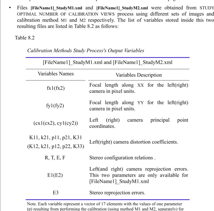
Table 8.2: Calibration Methods Study Process's Output Variables...64
Table 8.3: Stereo Calibration Process's Output Variables...65
Table 8.4: Rotation Parametrization Process's Output Variables...66
Table 8.5: Calibrated and Uncalibrated Rectification Process's Output Variables...66
Table 8.6: Recovering 3D Points Process's Output Variables...67
Table 8.7: L01 Set S03 Calibration Methods Study Using fx and k2 Parameters...68
Table 8.8: L02 Set S03 Calibration Method's Study Using fx and k2 Parameters...69
Table 8.9: L03 Set S04 Calibration Method's Study Using fx and k2 Parameters...70
Table 8.10: Stereo Calibration Parameters Optimization Results (L01, L02, and L03)...75
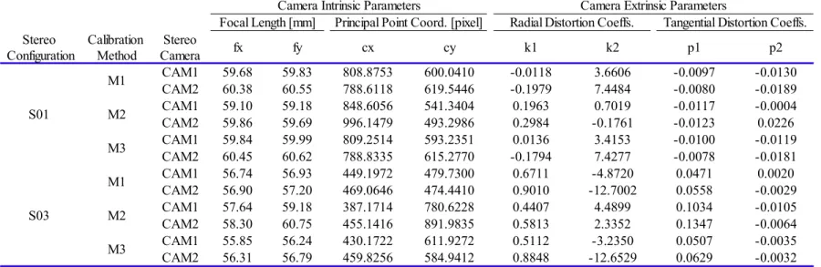
Table 8.11: Laboratory L01's Camera Calibration Parameters (Methods M1, M2, and M3)...78
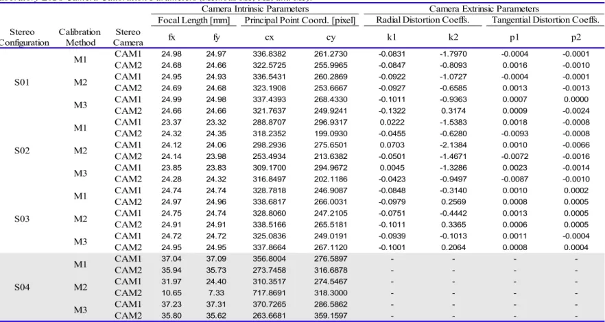
Table 8.12: Laboratory L02's Camera Calibration Parameters (Methods M1, M2, and M3)...79
Table 8.13: Laboratory L03's Camera Calibration Parameters (Methods M1, M2, and M3)...80
Table 8.14: Laboratory Stereo Configuration's Measurements...83
Table 8.15: Stereo Configuration's Relations ...83
Table 9.1: Calibration Method's Study Summary...89
4 Illustration Index
Figure 6.1: Relative errors vs. noise level (α, β), Zhang (2000)...16
Figure 6.2: Absolute errors vs. noise level (u, v), Zhang (2000)...17
Figure 6.3: Relative error vs. number of planes (α, β), Zhang (2000)...17
Figure 6.4: Absolute error vs. number of planes (u0, v0), Zhang (2000)...17
Figure 6.5: Relative error vs. angle with image plane (α and β), Zhang (2000)...18
Figure 6.6: Absolute error vs. angle with image plane (u0, v0), Zhang (2000). ...18
Figure 6.7: Parameter result's variations with different sets of images, Zhang (2000)...19
Figure 6.8: Calibration parameter's results with different image sets, Zhang (2000). ...19
Figure 6.9: Stereo matching process, Stefano et al. (2002)...29
Figure 6.10: Scores associated with point R(x, y), Stefano et al. (2002)...30
Figure 6.11: SAD matching window, Stefano et al. (2002)...31
Figure 6.12: Tsukuba image (left) and ground truth (right), Stefano et al. (2002)...34
Figure 6.13: Disparity maps computed with the P.A (left) and with SVS 2.0 software (right), Stefano et al. (2002)...35
Figure 6.14: Speed (fps) for P.A. and for the SVS 2.0 algorithm, Stefano et al. (2002)...35
Figure 7.1: Phantom v.91 cameras arranged on a stereo configuration. ...42
Figure 7.2: PCC1.2 software - cine settings...42
Figure 7.3: Targets used for points tracking purposes...43
Figure 7.4: PCC Software - save cine settings...46
Figure 7.5: StereoVisionProg: Main menu 's Option [ 2 ]...46
Figure 7.6: StereoVisionProg: Main menu's Option[ 2 ] sub Option [ 3 ]...47
Figure 7.7: Sequence of BMP images for calibration...47
Figure 7.8: StereoVisionProg: Main menu's Option [ 3 ] sub Option [ 1 ]...47
Figure 7.9: StereoVisionProg: Main menu's Option[ 3 ] sub Option[ 2 ] ...48
Figure 7.10: Reprojected (a) and projected (b) image points...49
Figure 7.11: Calibration parameters optimization process...50
Figure 7.12: StereoVisionProg: Main menu's Option [ 3 ] sub Option [ 4 ]...50
Figure 7.13: StereoVisionProg: rectification method options. ...50
Figure 7.14: Right camera rotation using Euler angles...53
Figure 7.15: Pseudo-code to compute quaternion from R. ...54
Figure 7.16: StereoVisionProg: Main menu's Option [ 4 ] sub Option [ 2 ]...55
Figure 7.17: StereoVisionProg: Main menu's Option[ 4 ] sub Option[ 2 ] sub Option[ 2 ]...55
Figure 7.18: Sparse stereo correspondence with Lucas-Kanade tracker. ...56
Figure 7.19: Canonical stereo configuration (a), similarity of triangles(b)...57
Figure 7.20: Camera-to-MELFA robot referential transformation...60
Figure 7.21: Referential transformation using point-line-plane method. ...61
Figure 8.1: L01-S03Focal Length vs Nº of Calibration Views (M1 and M2)...71
Figure 8.2: L03-S04 Focal Length vs Nº of Calibration Views (M1 and M2)...72
Figure 8.3: Single calibration view from L02 set S03 (a) and L03 set S04 (b)...72
Figure 8.4: L02-S03 Focal Length vs Nº of Calibration Views (M1 and M2)...73
Figure 8.5: L03-S03 Focal Length vs Nº of Calibration Views (M1 and M2)...73
Figure 8.6: Calibration parameters optimization (Method M3). ...74
Figure 8.7: Calibration view's reprojection/projected image points...76
Figure 8.8: Stereo video capture without rectification...81
Figure 8.9: Stereo video capture after calibrated stereo rectification...82
Figure 8.10: Stereo matching using Block-Matching algorithm...84
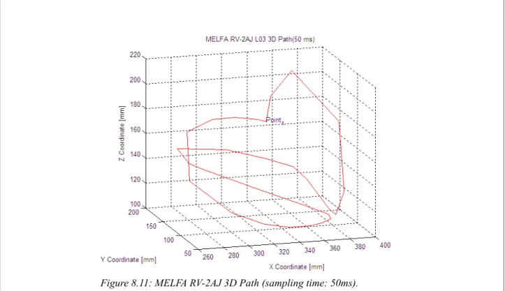
Figure 8.12: Figure 8.8: MELFA RV-2AJ 3D Path (sampling time: 10ms)...85
Figure 8.13: MELFA robot's recovered 3D path(camera coordinates system)...86
Figure 8.14: MELFA robot's recovered 3D path (robot coordinate system)...86
Figure 8.15: MELFA robot's recovered 3D path (generic coordinate system)...87
Figure 11.1: Pinhole camera model...100
Figure 11.2: Simplified pinhole camera model...101
Figure 11.3: Example of a 5-by-3 chessboard corner's detection. ...103
Figure 11.4: Generic point defined on a planar calibration object. ...104
Figure 11.5: Relation between a point in the planar object and the imager plane...105
Figure 11.6: Calibration object - chessboard 5-by-3...107
Figure 11.7: Building object point's vector of vector of 3D points...108
Figure 11.8: Stereo configuration geometry ...111
Figure 11.9: Standard stereo configuration's epipolar geometry. ...112
Figure 11.10: Video sequences after stereo rectification...117
Figure 13.1: Video Strobe - Flood Controller and 3-by-4 LED Array used during laboratory experiment 03. Adapted from VideoStrobe & VideoFlood LEDs by Visual Instrumentation Corporation 2009, Adapted with permission...142
Figure 13.2: LED Array specifications. Two 3-by-4 LED Array Model 900405 were used during laboratory experiment 03. Adapted from VideoStrobe & VideoFlood LEDs by Visual Instrumentation Corporation 2009, Adapted with permission...143
Figure 14.1: Phantom v. 9.1 Data Sheet p1/3. Adapted from Phantom v9.1 by Vision Research Inc, 2007. Adapted with permission. ...146
Figure 14.2: Phantom v. 9.1 Data Sheet p2/3. Adapted from Phantom v9.1 by Vision Research Inc, 2007. Adapted with permission. ...147
Figure 14.3: Record speed vs. Image Resolution p3/3. Adapted from Phantom v9.1 by Vision Research Inc, 2007. Adapted with permission. ...148
Figure 14.4: Mechanical shutter p1/2. Adapted from V-Series Lens Shutter by Vision Research Inc, 2010. Adapted with permission. ...149
Figure 14.5: Break-out-Box p2/2. Adapted from V-Series Lens Shutter by Vision Research Inc, 2010. Adapted with permission. ...150
Figure 16.1: Sequence of frames where the optical flow is to be computed...165
Figure 16.2: Normal flow. ...166
Figure 16.3: Aperture problem originated by a small aperture window...167
Figure 16.4: Result from applying the pyramid Lucas - Kanade technique...168
Figure 17.1: Dimensioning of the target1 and target 2...172
Figure 17.2: Dimensioning of the target 3. ...173
Figure 17.3: Targets 1, 2, and 3...174
Figure 17.4: MELFA Basic IV simple 3D path program implementation. ...175
Figure 18.1: StereoVisionProg: Main menu...177
Figure 18.2: Main menu's option 0 sub menu. ...178
Figure 18.3: Current directory's list of avi files...178
Figure 18.4: TRACKING SETTINGS window's trackbars...178
Figure 18.5: Sparse optical flow tracking example...179
Figure 18.6: Dense optical flow using Horn - Schunck method...179
Figure 18.7: Main menu's option 1 sub menu...180
Figure 18.8: Capture controls' window...180
Figure 18.9: OpenCV video compression selection...181
Figure 18.10: Main menu's option 2 sub menu...182
Figure 18.11: Capturing from two A4Tech Web Cams...182
Figure 18.13: Real-time stereo calibration. ...185
Figure 18.14: Main menu's option 3 sub menu...186
Figure 18.15: Study optimal number of calibration views...187
Figure 18.16: Calibration process method M1 and M2...188
Figure 18.17: Calibration parameters optimization...189
Figure 18.18: Calibrated stereo rectification...190
Figure 18.19: Uncalibrated stereo rectification...190
Figure 18.20: Main menu's option 4 video input...191
Figure 18.21: Stereo matching modes...191
Figure 18.22: Dense stereo matching approach...192
Figure 18.23: Block – Matching control window...193
Figure 18.24: Image points tracking settings...194
Figure 18.25: Sparse stereo matching approach. ...195
5 Chapter One
5.1 Introduction
The capability to perceive the three dimensional world where we live for us humans is a task that since the beginning seems easy and granted. It may take only two years for a baby be capable to experience the world through his senses such as looking, touching and even understanding that an object exist even when is hidden from the field of view (FOV). In the up following years he
become capable to represent the three dimensional world with colours, objects, shapes and symbols resulting from the four stages of cognitive development that we humans pass through (http://alleydog.com/psychology-topics.php, Child Psychology, ¶ 4 , 5).
Because we humans are provided with such complex and efficient human visual system (HVS) that does all the computations for us it may create a misleading impression that attempting to effectively simulate and copy such functions is an easy task. For perceiving the information gathered from HVS the brain uses three main principals: stereo vision, motion parallax and the prior
knowledge about the objects perspective appearance and their relation with the distance (May, Pervoelz, & Surmann, 2007), however, in machine visual systems the information is received from the sensing machine or a media storage and transformed into different layers of matrices numbers and in most cases without any previous knowledge about the surrounding variables (weather , lightning, reflections, occlusions, movements) that change the way images are captured and this is all the information available (Bradski, & Kaehler, 2008).
Computer Vision (CV) is the science challenged to study the transformation of that information in form of images or sequences of images into information that allows to implement and deal efficiently with all this three complex tasks for perceiving the 3D space by means of machine visual
sensing. This science has been widely progressing through the years since the time it started capturing the interest of researchers to mimic the human intelligence and reproduce it into the robots intelligence (Szeliski, 2010). However, it was manly in the recent decades that the interest by the researchers and the high demands from the industry for new features affordable by computer applications has notoriously increased.
Computer vision have been developing in parallel with common areas such as computer science, optical systems and mathematical techniques that with time are becoming more and more able to decode the inverse vision problem. Computer vision became a very vast field of studies but one field in special has received major attention in particular – the capability of performing effective automatic reconstruction and analysis of the surrounding 3D environment and objects recognition
in that space (Cyganek, & Siebert, 2009).
In addition to the fast development in computer vision, new ways of commercialization gives origin to performance-optimized software that runs in different platforms and that are mostly open source free for both academic and commercial use what makes easy to exchange experiences and documentation widely among research groups and therefore providing a base for a faster development. One example of this strategy is the case of Intel with the Open Source Computer Vision (OpenCV) that provides computer vision applications to increase the need for faster processors (Bradski et al. 2008).
OpenCV is a library of programming functions mainly directed for real time computer vision such motion tracking, stereo and multi-camera calibration and depth computation (http://opencv.willowgarage.com/wiki/FullOpenCVWiki, Introduction ¶ 1). This capabilities offered by OpenCV combined with the object-oriented and generic programming techniques
offered by C++ programming language is a suitable choice to implement large and reusable
projects (Papademetris, 2006).
To recover the information lost on the process of projecting 3D world space to the 2D image space the implementation of a number of classes objects is an essential part for the recovering process. This process requires the successful implementation of a program capable to calibrate two cameras with equal properties, capture stereo-pair images of a scene and then compute the depth information within those two images and reproject it to 3D space in real time, by means of using
OpenCV libraries and C++ object oriented programming (OOP) capabilities.
5.1.1 Statement of the Problem
The challenges present in recovering the 3D information from 2D images based on processing
stereo-pair images are related to three main areas: cameras calibration, images rectification, disparity maps and its reprojection to 3D space. To achieve the so desirable information in
three-dimensional space from a sequence of stereo-pair images it is necessary to recall the basic principles that are crucial to its correct implementation.
Firstly to determine the coordinate transformation between the camera reference system in respect to an external coordinate system, it is necessary to know the variables that relates such relation. The direct measurement of those variables is difficult or even impossible and therefore a process of calibration is required to determine camera intrinsic and extrinsic parameters. The final performance of the machine vision system strongly depends on the accuracy of camera calibration (Niola, Rossi, Savino, & Strano, 2008). The information retained by the extrinsic parameters are used to correct the distortion induced by the hardware, this process is called undistortion.
Ideally cameras' arrangement would be such that the resulting images are row aligned and each point of one image will correspond to another point in the same row of a second image, however such canonical stereoscopic system is not possible physically and the images need to be remapped, this process is referred to as rectification.
The last challenge on the process of recovering the lost dimension requires the correspondence process. Simply stated, correspondence refers to the matches between two images captured from two different viewpoints looking at the same 3D world scene or object. It is one of the most active
topics in computer vision due its complexity and important role in 3D object recognition and categorization, scene reconstruction and many other applications (Hsu, 2011).
5.1.1.1 Correspondence.
One of the major issues on estimating 3D structures based on stereo imagery is the
correspondence problem defined as the capability to locate a pair of image pixels from two different images that represent the projection of the same point in 3D space. Given a point in one
image, its correspondent point must lie on an line (epipolar line) in the other image. This constitutes a very important constraint called epipolar constraint: Each image point of a space point lies in the image plane only on the corresponding epipolar line (Cyganek et al., 2009). This constraint presents a second problem, in general cases the location of the epipolar lines are not known.
5.1.1.2 Rectification.
As stated previously the positions of the epipolar lines are not known for a standard stereoscopic camera configuration however for the canonical stereoscopic configuration those lines positions can be know using epipolar geometry and thus this transformations between the generic configuration to the desired canonical configuration constitutes the second problem of the research
area. In order to perform successfully this operation between both configurations previous knowledge is required to know how the cameras related the world coordinates with the image coordinates when capturing the images or sequence of images. This process is referred to as
camera calibration (Shah, 1997).
5.1.1.3 Camera Calibration.
Camera calibration is the first problem to be solved and it plays an important role in the final results on the research area. Camera calibration is the process to estimate a set of parameters that describes the camera imaging process. Computing this set of parameters will allow to: link directly a point in the 3D world reference frame to its corrected image through the perspective projection
matrix (Ma, Chen, & Moore, 2003) , map the camera coordinate system into the image coordinate system, and compute geometrical distortions that are originated by the imperfections and limitations of camera's physical parameters (Cyganek et al., 2009).
As noted, recovering the lost dimension to estimate 3D structures based on stereo images requires that three steps need to be successfully implemented. Initially the camera model, the distortions and perspective projection matrix are computed. This step is important once the accuracy in which the de camera parameters were computed will play an important role in the final depth results. In order to obtain two images with stereoscopic camera configuration and simplify the mathematical relations a process of rectification is performed on both images so they become as if the cameras where in the canonical configuration with the optical axis meeting at infinity. Finally in order to compute the depth images using the both rectified images a correspondence process is performed and the third dimension recovered from the image coordinates where was possible to match both image pixels (Wu, & Chen, 2007).
5.1.2 Background and Need
The earliest techniques for reproducing 3D information using stereo matching approach started
in the area of cartography for automatic construction of topographic elevation maps from overlapping aerial images. This initial progress in the aerial imagery area played an important role in the progress and development of fully automated and efficient stereo matching algorithms in depth recovering field (Szeliski, 2010). However, since computer vision started out in the early 1970s many attempts to recover the three-dimensional structures happened in parallel with a wide area of studies as the case of stereo vision techniques and algorithms and cannot be seen as a separate issue. Szeliski (2010) provides a good and detailed synopsis of the main developments in computer vision over the last 30 years, as well a rich number of references used along the text for the researcher that wishes to go deeper in any particular subject.
In the context of stereo vision and depth recovery, in many cases, the overall performance of the machine vision system strongly depends on the accuracy of the camera calibration. Camera calibration is the process of determining camera geometric and optical characteristics and the 3D
position and orientation of the camera frame relative to an external world frame (Heikkila et al., 1997). The epipolar geometry is implicitly connected with the pose and calibration of the stereo cameras, once this geometry is computed the epipolar line corresponding to a pixel in the left image can be used to constrain the search for a corresponding pixel in the right image.
Stereo vision besides being studied for long time it is still considered a mature technology. Recovering depth information requires great performance since pixel correspondence from left image to the right image need to be found what can be challenging if the images are from very
different viewpoints or contains noise, occlusions, homogeneous regions or unpredictable environment light conditions that makes it difficult, moreover depth based applications such as navigation for mobile robots requires high efficiency for a real-time response what makes it even more challenging (May et al., 2007).
Research problem: Recover of the 3D information lost in the process of projecting a 3D scene into an 2D image with OpenCV image processing platform.
5.1.2.1 Camera Calibration.
• Problem: Internal camera geometric and optical characteristics (intrinsic and extrinsic parameters) as well as the 3D position and orientation of the cameras frame relative to an
external coordinate frame and relative to each other camera coordinates are unknown in a standard stereoscopic configuration.
• Solution: Algorithm for calibrating a camera with possibly variable intrinsic parameters and position, that copes with an arbitrary number of calibration planes and camera views. Calibration is achieved by projecting the planar calibration object into 2D image, each
projection contributes with a system of homogeneous linear equations in the intrinsic parameters which are easily computed by solving the linear equations (Sturm, & Maybank, 1999).
5.1.2.2 Rectification.
• Problem: Canonical stereoscopic configurations are rare with a real stereo system since the two cameras almost never have coplanar and row-aligned imaging planes as desired for a more reliable and computationally efficient stereo correspondence.
• Solution: Reproject the image planes of the two cameras so that the epipolar line with the conjugate epipolar line become coincident with the horizontal scan-line reducing stereo matching from a 2D to a 1D search (Bradski et al., 2008).
5.1.2.3 Correspondence.
• Problem: Stereo analysis is the process of retrieving the depth information based on the 3D
object/scene projection on two or more images. Finding corresponding pixels between both images or sequence of images constitutes the stereo analysis fundamental problem.
• Solution: Use a fast and effective area-based stereo matching algorithm that compares each small area with other area in a search window and then determines the extreme value of the correlation at each pixel resulting in a value that holds the disparity value between the left and right image patches at the best match that will result in a final disparity image (Konolige, 1997, Bradski et al., 2008).
The literature solutions previously described are strictly connected with their implementation in the OpenCV Image processing library what provides a better tool for a new researcher in this field. However due the vast number of research areas in the computer vision field and it fast progress in the last decades the need for standardization and definition of each individual research area within this field is needed for a better overall understanding. For a new researcher in this field of studies the literature still is one of the main obstacles for a fast learning curve. The link between the scientific and statistical approaches (vision analysis and formulation) and the engineering approach (algorithms implementation) constitutes the literature main gap (Szeliski, 2010). A better
explanations about the image programming languages available, their advantages and disadvantages as well as a methodology to analyse the efficiency and cost of the huge number of existing algorithms are also needed in the current literature.
5.1.3 Purpose of the Study 5.1.3.1 Purpose Statement.
The purpose of this study was to utilize the OpenCV image processing platform together with Microsoft Visual Studio 2008 software to implement a program for recovering 3D information from
video sequences captured with two Phantom v9.1 cameras arranged on a stereo configuration. 5.1.3.2 Need/Rationale for the Study.
In the recent decades the concept of Open Source has been increasing gradually captivating the interest of professionals and young researchers in the different areas. OpenCV image processing platform for computer vision is not exception and has been assisting to a great acceptance by the researchers community. Due the numerous functionalities it provides and the good documentation as well a vast community that can interact and provide fast answers, it was the image processing platform chosen to conduct the study. Stereo Vision is the computer vision area that during the last decades has gained special focus due its capacity to recover the depth information from two or more images. It is widely used in different applications such as surveillance, agriculture, mobile robotics, manufacturing and medical image analysis. This wide range of possible applications allied with the constant progress in innovative algorithms and increasing demand on the 3D
computer graphics constitutes one of the main reasons to conduct the study using stereo vision approach.
5.1.3.3 Description of the Study.
In order to recover the depth from stereo video sequences, the researcher made use of OpenCV algorithms to implement a program with different stereo functionalities. This program studies the optimal number of calibration views needed, computes camera calibration using two methods and performs calibration optimization by excluding calibration views with higher error contributions. Calibrated and uncalibrated rectification methods were implemented in order to obtain the remapping maps and the disparity-to-depth matrix using different approaches. To recover the depth from stereo video sequences two methods were implemented: the first method used the stereo matching algorithms available from OpenCV libraries namely the Block Matching, Semi Global Block Matching, and Graph Cut algorithm to compute disparity images and then reproject it to 3D
space, or the second method that made use of Lucas – Kanade Pyramid tracker code and mouse click event to track a set of points of interest over a stereo video sequence, compute its disparity and compute their corresponding 3D points related to the left or to the right camera coordinate
system. Stereo video sequences were captured using two Phantom v9.1 high-speed cameras arranged on a standard stereo configuration. Different stereo configurations were used to record video from a calibration pattern and later from a MELFA RV-2AJ robot's end-effector movement. All
the research output results were stored in xml file formats with proper nomenclature depending on which stereo operation was performed.
5.1.3.4 Expected Outcomes.
The expected outcomes of this case study are to develop programming skills using a C++ object oriented approach together with the newer and more efficient OpenCV C++ interface. By implementing a main program to deal with 3D points recovering it is expected to obtain a number
of ready-to-use classes capable to read a list of calibration views and AVI files, compute calibration
parameters and stereo relations and optimize those results, undistort and remap stereo video captures from a standard stereo configuration and recover the depth of a captured scene (disparity image) or sparse set of points from the available stereo video sequences. Another goal of the study was to provide a more practical approach through laboratory experiments with two Phantom v9.1 cameras which it is expected to develop a better understanding how stereo configuration's settings, capture settings and environment settings influences the outputs results obtained from the captured video sequences for stereo calibration and 3D information recovering purposes.
5.1.4 Research Questions
1. Which are the OpenCV main functions involved in the process of: stereo camera
calibration, stereo image rectification, stereo matching and points reprojection into 3D space, and Lucas – Kanade Pyramid optical flow method. What are the inputs and outputs arguments of those functions.
2. How to compute camera calibration parameters using a planar calibration object known as chessboard and how to relate two cameras in a stereo configuration. How many calibration views are needed to perform the stereo calibration process and which calibration method (with and without initial guess to compute stereo relations) gives better results. How to optimize the stereo calibration process and improve the calibration parameters results.
3. Which are the differences between using calibrated and uncalibrated rectification methods and how to implement the image rectification process by means of using OpenCV functions. 4. How to parametrize the stereo relation's rotation matrix into Euler angles and quaternions
and how to perform the transformation between this two rotation representations.
5. How to compute the disparity image and disparity of a sparse set of points given two
rectified images captured from a stereo configuration previously calibrated. How to reproject a sparse set of points to the 3D space.
5.1.5 Significance of the field
The contributions resulting from this study to the research literature were various. By using the OpenCV libraries' algorithms this case study provides a number of functionalities to work with video capture and video recording operation, capture and list stereo images for calibration purposes or perform simple tasks such as images colour space transformation or frame saving operations using different image formats. Related with the calibration process a number of functions were implemented within a class to allow single or stereo cameras calibration process using a text file with a list of calibration views to be loaded or alternatively it allows to perform the calibration process directly from AVI video files or real time video capture. Additionally was implemented a
method that by excluding bad views used in the calibration process and recalling the calibration process again it allows to optimize substantially the final calibration parameters and reduce the reprojection errors. To perform the uncalibrated and calibrated stereo rectification after each stereo calibration process was implemented another class that can be easily reused in the future research. An additional class was built with functions that allows to capture video sequences from stereo
cameras or stereo AVI files and remap the images to compute the dense disparity image or the
disparity for a sparse set of points and then proceed with the reprojection to 3D space. The case
study will also provide conclusions and knowledge achieved during the laboratories experiments, as well the procedures' changes that allowed to improved substantially the calibration and 3D
recovering results. 5.1.6 Definitions
• fx , fy : Camera focal length in pixel units on XX and YY direction, respectively.
• R : Stereo relation 3-by-3 rotation matrix that brings (rotates) the right camera to the left camera orientation.
• Q : Disparity-to-depth transformation matrix used to reproject 2D image points to 3D
world space.
• D1(D2) : Left (right) camera distortion coefficients vector D=[ K1K2p1p2K3]T where K1,K2 and K3(only for wide−anglelenses) are the radial distortion coefficients and ( p1,p2) the tangential distortion coefficients.
• L01 , L02 , L03 and S01 , S02 , S03 , S04 : Nomenclature used to identify the different stereo video sets (S01, S02, S03, and, S04) recorded during the three laboratory sessions (L01, L02, and L03). If the nomenclature is used in the calibration context it refers to the video sequences captured for calibration purposes otherwise it refers to the video sequences captured for recovering 3D information purposes.
• cx , cy : Principal point coordinates in pixel units.
• map1x, map1y(map2x, map2y) : Remapping maps for the left (right) camera's video
capture that are used to perform the (undistortion+rectification) transformation. • T : Stereo relation translation vector T =[TxTyTz]
T
that brings (translates) the right camera to the left camera position.
• Camera calibration: Process of finding the camera intrinsic and extrinsic parameters such as focal length, principal point and lens distortion parameters.
• Camera Matrix: Projective transform matrix that relates the real world coordinates to the points on the image plane.
• Canonical Stereo Configuration: Stereo configuration where the cameras' imager are ideally coplanar and row aligned.
• CSR: Current Session Reference available from phantom camera control software. • CV: Computer Vision.
• Disparity: The difference between two image points, representing the same 3D point in the
world scene, within two stereo images.
• E: Essential matrix: Contains information about the rotation and translations that relates
the two cameras on the stereo configuration.
• Epipolar geometry: The geometry relations between the 3D points and their projections into the 2D image planes that form a number of constraints between two stereo images'
• Epipolar line: Is the line formed by the epipolar plane's intersection with the camera's imager plane.
• Epipolar plane: Is the plane passing through an object point and the cameras' centres of projection.
• Euler angles: describe the rotations that moves a rigid body from one referential to another with different orientation by using only three parameters (yaw, pitch, roll).
• Extrinsic parameters: Are the parameters that define the camera's position and orientation (three rotation
(Φ
,Θ , Ψ )
and three translation(
T
x, T
y,T
z)
parameters) with respect to a known 3D world reference frame.• F: Fundamental matrix that relates the two cameras, on a stereo configuration, in pixels
coordinates.
• Focal Plane: The plane in a camera, or other optical instrument in which a real image is in focus.
• HVS: Human Vision System.
• IDE: Integrated Development Environment.
• Intrinsics parameters: Are the parameters that define the camera's optical and geometric characteristics such as the focal length, the principal point coordinates and the radial and tangential lens distortions.
• Lens Distortion: Lens imperfections that introduces distortions on the image's pixel locations.
• Occlusions: Regions that are originated by disparity discontinuities. • OOP: Object Oriented Programming.
• OpenCV: Open Source Computer Vision Programming Library.
• Optical flow: Is the velocity field in the image plane resulting from the motion of the objects being observed, the motion of the observer, or apparent motion which may be caused by changes in the image intensity between frames.
• PCC: Phantom Camera Control software.
• Planar Calibration Object: Object used to capture images for camera calibration purposes using OpenCV algorithms.
• Principal Axis: Line that passes through the lens curvature's center, also known as optical axis.
• Principal Plane: Plane that is perpendicular to the lens optical axis.
• Principal Point: Point that results from the intersection of the image plan and the optical axis.
• Quaternions: Mathematical notation for representing rotations and orientations of objects or frames in 3D space.
• SDK: Software Development Kit.
• Standard Stereo Configuration: The real stereo configuration where the cameras' imager are not ideally coplanar or row aligned as in the canonical configuration.
• Stereo Correspondence: The process of matching image points from two different images, captured from a stereo configuration, that represent the same object points on the 3D world space.
• Stereo Rectification: Relates the two cameras in the space by means of rotations and translations and the result are pair of images row-aligned and rectified.
• StereoVisionProg: Researcher-made program implemented to answer the proposed research questions.
• STL: Standard Template Library.
• UML: Unified Modeling Language.
• Undistortion: Process of computing undistorted images (corrected images) by mathematically removing radial and tangential distortions.
5.1.7 Limitations
The limitation of this research are mainly inherent to the data analysis and time limitations. The time available to make this research was exceptionally short for a complete and solid review of the extensive stereo imagery literature as well to learn the C++ programming language and to obtain a complete familiarization with the OpenCV algorithms. Due the lack of time, the initial purpose for implementing an interface able to interact with the Phantoms v9.1 cameras using the Phantom SDK was not implemented which constitutes also a limitation in this study.
In what concerns to the dense stereo matching methods the research design adopted did not included other stereo matching algorithms besides the ones available from OpenCV 2.1 libraries, the study also did not included any comparison related with speed and computational cost between those stereo matching algorithms, this limited the conclusions obtained from dense stereo matching and the possibilities to obtain better disparity images.
6 Chapter Two
6.1 Review of the Literature
6.1.1 Introduction
The world we humans daily perceive is the 3D world, but the images captured from it are 2D, one dimension is lost in the capturing process. One important task in the Computer Vision field is to recover back the third dimension (Shah, 1997). There are several methodologies to recover the
3D information from 2D images, one of them widely studied in computer vision is the stereo imagery approach. In stereo imagery approach two images ( left and right ) are used to recover the depth information. The depth recovery relies on three main areas: the first consists on capturing a number of image pairs of a planar object that will be used to calibrate both cameras, this area is termed as calibration. The second area consist on correcting and remapping each pixel on both images in such a way that the images are suitable to apply matching algorithms, this area is termed as rectification. Finally after applying the calibration and rectification processes, respectively, a third step need to be performed to compare and compute the disparity maps, this area is termed as correspondence.
The literature review will address three areas related to the depth recovery using stereo imagery. The first section will address research related to the cameras calibration. The second section will focus on research studies about the images rectification. Finally the third section will discuss research related to stereo correspondence problem.
6.1.2 Research Synthesis
6.1.2.1 Camera calibration review. • Introduction
One of the main goals of computer vision is to understand the visible world by inferring
3D properties from 2D images (Jiang, & Zhao, 2010). In the context of stereo imagery the
first step that need to be performed in the process of recovering 3D information from 2D
images is known by the term calibration. Camera calibration is the process of computing the internal camera geometric and optical characteristics and modelling the relationship between 2D images and 3D world.
A large number of calibration methods are presented in the literature. The literature suggest that this methods can be characterized in three main categories: traditional methods, self-calibration and the active-motion based methods. The former method, the one that will be reviewed, is performed by observing a calibration object whose exact geometry in 3D
space is known with precision. This method provided by Zhang (2000) was particularly of the research interest once it provides similar methodology to the one implemented by OpenCV platform, as well a common ground for data comparison.
• Purpose
calibrate a camera by observing a planar pattern shown at at least two different orientations. Either the camera or the planar pattern can be freely moved without the need to know the motion (Zhang, 2000).
• Methods
The calibration is performed by observing a planar calibration object whose geometry is known in 3D world with good precision. This methodology avoids the use of expensive calibration apparatus such the ones based on three coplanar planes or diffractive optical elements, instead it uses a pattern that can be easily printed on a laser printer and attached to a planar surface. Either the camera or the calibration object can be moved by hand to provide a rich set of pattern orientations.
Calibration Procedure. This section will provide the formulation to compute the camera
calibration parameters. Firstly it presents the notation and the planar homography, then the analytical solution followed by a non linear optimization without and with lens distortion effects and finally the procedure summary.
Notation
A 2D point is represented by m=[u , v ]T and a 3D point is represented by M =[ X , Y , Z ]T , m̃ and M̃ denote the augmented vector by adding 1 resulting in:
̃
m=[u , v ,1]T , M =[ X ,Y , Z ,1]̃ T respectively. The camera is modelled by the pinhole model. The relation between the 3D point M and its image projection m is:
s ̃m=A[ R t] ̃M
(6.1.1)
With A=[
α c u0 0 β v0 0 0 1]
.The extrinsic parameters are the rotation and the translation (R ,t ) that relates the world coordinate system to the camera coordinate system. A Is the camera intrinsic matrix and
(u0, v0) are the coordinates of the principal point. The α ,β are the scale factors along
u , v image axis, and c the skewness of the two image axes.
Along the article A−T is used in place of (A−1
)T, or( AT)−1 .
Planar Homography
Without lose of generality, the model plane is assumed to be on Z =0 world coordinate system. Denoting the ith column of the rotation matrix R by r
i . From equation
(6.1.1), is possible to obtain the following relation:
s
[
uv 1]
=A[
r1 r2 r3 t]
[
X Y 0 1]
=A[
r1 r2 t]
[
X Y 1]
Since Z =0 for all the planes, M was redefined to denote a point on the model plane
m is related by a homography H :
s ̃m=H ̃M (6.1.2)
With H = A
[
r1r2t]
. The 3-by-3 matrix H is defined up to a scale factor.Intrinsic Camera Parameters Constraints
Given an image of the model plane, the planar homography can be estimated. Denoting it by H =
[
h1h2h3]
and by substitution in equation (6.1.2) the following relation was obtained:[
h1h2h3]
=λA[
r1r2t]
, where λ=1/ s . Given an homography and using the knowledge that r1and r2 are orthonormal vectors, two basic constraints on the intrinsic parameters are obtained :h1TA−TA−1h2=0 (6.1.3)
h1TA−TA−1h1=h2TA−TA−1h2 (6.1.4) Because a homography has 8 degrees of freedom and there are 6 extrinsic parameters (3 for rotation and 3 for translation), only 2 constants can be obtained on the intrinsic parameters.
Solving Camera Calibration
Once presented the notation and planar homography, this section summarize the article methodology to solve the camera calibration problem. Firstly was presented the analytical solution followed by a non linear optimization technique and finally the consideration of radial distortion in the calibration process.
Closed-form solution. Let B=ATA1 ≡
[
B11 B12 B13 B12 B22 B23 B13 B23 B33]
(6.1.5) B=[
1 α2 − c α2β c v0−u0β α2β − c α2β c2 α2β2+ 1 β2 − c(c v0−u0β) α2β2 − v0 β2 c v0−u0β α2β − c(c v0−u0β) α2β2 − v0 β2 (cv0−u0β) 2 α2β2 + v0 2 β2+1]
B is a symmetric matrix defined by 6D vectorDefining the ith column vector of H as h
i=
[
hi1hi2hi3]
Tthen a new relation is obtained:
hiTB hj=vijTb (6.1.7)
With vij=
[
hi1hj1, hi1hj2+hi2hj1, hi2hj2, hi3hj1+hi1hj3, hi3hj2+hi2hj3, hi3hj3]
T . Therefore the two fundamental constraints (6.1.3) and (6.1.4), from a given homography, can be rewritten as 2 homogeneous equations in b:[
v12T(v11−v22)T
]
b=0 (6.1.8)If n images of the model plane are observed, by stacking n such equations as (6.1.8) a new relation is obtained:
Vb=0 (6.1.9)
Where V is a 2n – by – 6 matrix. If n⩾3 a unique solution is obtained up to a scale factor.
If n=2 , the skewness constraint can be imposed to be zero, c=0 , i.e. an additional equation
[
0,1,0,0,0,0]
b=0 is added to the equation(6.1.9).The solution to equation (6.1.9) is known as the eigenvector of VTV associated with the smallest eigenvalue. Once b is estimated, the camera intrinsic matrix A and the extrinsic parameters can be computed. From equation (6.1.2) the rotations and translation can be easily obtained:
r1=λA−1h1, r2=λA−1h2, r3=r1×r2 and t=λ A−1h3 with λ=1/
∥
A −1h1 or2
∥
.Additional computation needs to be performed in the returned matrix in order to solve the best rotation matrix R, i.e. the one that satisfy a rotation matrix requirements.
Maximum likelihood estimation
Given n images of a model plane containing m points and assuming that the image points are affected by independent and identically distributed noise the maximum likelihood estimate can be obtained by minimizing an algebraic distance which is not physically meaningful. This is done by minimizing the following equation:
∑
i=1 n∑
j =1 m ∥mij− ̃m(A , Ri, ti, M j)∥ 2 (6.1.10)Where m( A , R̃ i,ti, Mj) is the projection of point Mj in image i , according to
equation (6.1.2). The rotation R is parametrized by a vector r of 3 parameters which is parallel to the rotation axis and with magnitude equal to the rotation angle. R and r Are related by the Rodrigues formula. The non linear minimization problem of equation (6.1.10) is solved with Levenberg - Marquardt algorithm.
Considering Radial Distortion
The previous steps of this article did not took in account the lens distortion. This section will summarize the methodology used to estimate the camera intrinsic and extrinsic parameters considering the first two terms of radial distortion.
Let (u , v ) be the ideal or distortion-free pixel image coordinates and (̆u , ̆v) the corresponding real observed image coordinates. Similarly the (x , y ) and (̆x , ̆y) are the ideal or distortion-free and real or distorted normalized image coordinates, thus the real pixels are given by:
̆
x =x+x [ K1(x2+y2)+K2(x2+y2)2] ̆y= y+ y [K1(x2+y2)+K2(x2+y2)2]
where K1 and K2 are the coefficients of the radial distortion. The center of radial distortion is the same as the point formed by the intersection of the principal ray with the image plane (principal point) . Given the relation u=ŭ 0+α ̆x+c ̆y and ̆v=v0+β ̆y , the real image coordinates are given by the following equations:
̆
u=u+(u−u0)[K1(x2+y2)+K2(x2+y2)2] (6.1.11)
̆
v =v+(v−v0)[K1(x2+y2)+K2(x2+y2)2] (6.1.12)
The method to compute both distortion parameters assume that initially this parameters are small and thus ignored to compute the five intrinsic parameters. Then the method estimates
K1 and K2 based on those five parameters. From (6.1.11) and (6.1.12) each point in the
image is constrained by two equations:
[
(u−u0)(x2 +y2 ) (u−u0)(x2 +y2 )2 (v−v0)(x2 +y2 ) (v−v0)(x2 +y2 )2][
K1 K2]
=[
̆ u−u ̆ v−v]
Given m points in n images, all the equations are joined to obtain a system of 2mn total equations. This system of equations can be presented as
DK =d where K =[K1,K2]T . The linear least-squares solution is obtained by:
K =( DTD)−1DTd (6.1.13)
After solving the system of equations and obtained the values of K1 and K2 the solution for the previous five intrinsic parameters can be refined by solving equation (6.1.10) with the two new distortion parameters taken in account. Similarly to equation (6.1.10) the new set of parameters are estimated by minimizing the following functional:
∑
i=1 n∑
j =1 m ∥mij− ̃m(A , K1,K2,Ri, ti, Mj)∥ 2 (6.1.14)Where ̃m( A , K1, K2, Ri, ti, Mj) is the projection of point Mj in the distorted image
i , according to equations (6.1.2) , (6.1.11) and (6.1.12). The non linear minimization is solved in the same way as demonstrated previously for calibration neglecting lens distortion. The literature suggest that a second approach can be done to initially estimate the
K1 and K2 values by simply setting them to zero.
Procedure Summary
The researcher of this article recommend the following procedure: 1. Print a pattern and attach it to a planar surface.
2. Take a set of images from different orientations by moving either the camera or the model plane.
3. Identify the points of interest in the image.
4. Estimate the five intrinsic and extrinsic parameters neglecting radial distortions. 5. Estimate radial distortions coefficients by solving the linear least-squares equation
(6.1.13).
6. Recompute all parameters by minimizing equations (6.1.14). • Variables and Data Analysis
This article presents two distinct analysis. In the first part the article presents the computer simulated analysis for the algorithm performance with respect to the noise level, number of planes and the orientation of the model plane while the second part uses real data to analyse the influence of the number of planes in the intrinsic parameters and the influence of including the distortion coefficients on the refinement of those parameters.
Simulated Data Analysis
The camera matrix used (notation of equation (6.1.1) ) was:
A=
[
1250 1.09083 2550 900 2550 0 1
]
.
The pattern has a size of 18cm x 25cm containing 10 x 14 corners points with an image resolution of 512 x 512.
Algorithm performance varying the noise level. Three planes are used with the following
orientations and positions, respectively:
r1=[20º ,0,0 ]T, t1=[−9,−12.5,500]T r2=[0,20 º , 0]T,t2=[−9,−12.5,510]T r3= 1
√
5[−30º ,−30º ,−15º] T,t 3=[−10.5,−12.5,525]TGaussian noise with 0 mean and standard deviation is added to the projected image points. An 100 independent trials is performed by varying the noise level from 0.1 to 1.5 pixels. The relative error for α and β are measured as well the absolute error for u0 and v0 .
Algorithm performance varying the number of planes. This section investigates the
algorithm performance varying the number of images of the model plane. The number of images vary from 2 to 16. For the first three images the orientation and position of the model plane are the same as in the previous section and from the fourth image a rotation angle of 30º is applied to an arbitrary rotation axis. For each number, 100 trials of independent plane orientations and independent noise with mean 0 and standard deviation 0.5 pixels are conducted.
Algorithm performance varying the orientation of the model plane. This section study the
influence of the model plane orientation with respect to the image plane. The plane is initially parallel to the image plane and a rotation axis is chosen arbitrarily and the plane is
then rotated around that axis by an angle θ that varies from 5º to 75º. Gaussian noise with mean 0 and standard deviation 0.5 pixels is added to the projected image points. The process is repeated 100 times and the average error are computed.
Real Data Analysis
In the practical part of the study the images were captured with a PULNiX CCD camera 6
mm lens with 640x480 resolution. The model plane used a pattern of 8x8 squares with a a size of 17 x 17 cm. Five images from different orientations were taken.
The algorithm was applied to sets of different number (2,3,4,5, respectively) of images and the intrinsic camera parameters were measured first neglecting the lens distortion and secondly by using the maximum likelihood estimation(MLE) after including the radial distortion coefficients effects. The estimated standard deviation was computed for each intrinsic parameter and distortion coefficients as well the root mean square (RMS) for each
set of images. A second approach was implemented in order to study the stability of the proposed algorithm by applying the algorithm to all set of images combinations. The mean and deviation were computed for each intrinsic parameter and distortion coefficients as well the RMS for each combination.
• Results
The results returned by this study are summarized in two categories: The results concerning to the simulated data and the results concerning to the real data.
The results obtained for the simulated data are firstly discussed and presented in the same order. All the figures here included were adapted from this article.
From Figure 6.1 and 6.2 is possible to conclude that both errors increase linearly with the noise level. Taking in account that in real cases the noise is normally lower than 0.5 (
σ⩽0.5 ) the errors for α and β for that level of noise are smaller than 0.3%. In the case of u0 and v0 the errors are less than 1.5 pixels however v0 presents a lower error that for the same noise value that is less than 1 pixel due the fact that the pattern has more corners along v direction than in u direction. To have similar comparison a square pattern should be used.
From Figure 6.3 and 6.4 the relative error of both scale factors ( α and β ) decrease significantly as the number of planes increase and tends to stabilize for a relative error around 0.25% for a number of images greater than 11.The principal point coordinates error curves present the same tendency with a vertical displacement between them due difference in the number of samples as already mentioned above in the noise results.
Figure 6.2: Absolute errors vs. noise level (u, v), Zhang (2000).
Figure 6.3: Relative error vs. number of planes (α, β), Zhang (2000).
From Figure 6.5 and Figure 6.6 is possible to conclude that all parameters have minimum errors for angles within an interval of [40º; 60º] . The higher errors occur for small angles where the planes are almost parallel to each other and do not provide additional constraints on the camera intrinsic parameters (degenerate configurations). This occurrences, for some calibration algorithms, introduces numeric instability and can make the solution diverge to wrong results.
• Real data results
The algorithm results using real data are showed in Figure 6.7 and 6.8. Figure 6.7 shows the calibration parameters results using sets of 2, 3, 4 and 5 images. The “initial” column are the values obtained for the case were radial distortion was neglected and the “final” column are those parameters refined after estimate radial distortion coefficients
K1 and K2 , the third column ( σ ) is the estimated standard deviation. From this third
column is possible to conclude that the parameter values do not present significant differences in each set and the standard deviation converges rapidly by only increasing the number of images from 2 to 5. Figure 6.8 shows the combinations of all sets of images. The mean and sample deviation are showed in the last columns. The higher deviation occurs for the scale factors ( α and β ) but still considerably small what shows that the algorithm proposed is stable. The aspect ratio ( α /β ) was also computed for each combination and its mean and sample deviation are 0.99995 and 0.00012, respectively. The value very close to 1 shows that the camera CCD used was square, i.e. the sizes ( sx and sy ) of the
individual imager element are equal.
Figure 6.5: Relative error vs. angle with image plane (α and β),
Zhang (2000).
Conclusions/Implications
The algorithm proposed in this article provides an easy and flexible method to calibrate a camera by capturing images either moving the camera or the pattern plane. From the simulated data few conclusions can be done: better results are obtained for a rich set of images, i.e. with distinct orientations for angles within an interval of [40º; 60º] , images that only differ in position (pure translation) do not contribute with any additional information, and for a number of image planes greater than 11 the parameters errors are approximately constant. The real data computation also allows to conclude that the algorithm do not require a big number of images, the algorithm converges rapidly.
The proposed technique is flexibly, reliable and do not requires large number of images neither very expensive or elaborated calibration objects making it easy to use. It present the methodology also used by the OpenCV calibration functions used along this study.
Weakness/Limitations
This paper do not mentions explicitly any kind of limitations however some of its assumptions constitutes few limitations. The method assumes that the radial distortion function is mostly dominated by the first two terms however it is not partially true for wide angle or fish-eye lens types where the third coefficient has significant weight. The method did not establish an interval for the angle of rotation that gives the better results or studied the influence of higher angles (closer to 90º) vs. corners detection precision. Another limitation of this paper is due the fact it does not provide results with different patterns varying the number of corners and their sizes and the influence that this changes may cause in the calibration parameter results. Finally the fact of using rectangular patterns (ncornersalong u≠ncorners along v) did not allowed to compare directly the principal point coordinates for different noise levels (Figure 6.2).
Figure 6.7: Parameter result's variations with different sets of images, Zhang (2000).