Detection of outliers in multivariate data:
a method based on clustering and robust estimators
Carla M. Santos-Pereira1 and Ana M. Pires2
1 Universidade Portucalense Infante D. Henrique, Oporto, Portugal and
Applied Mathematics Centre, IST, Technical University of Lisbon, Portugal.
2 Department of Mathematics and Applied Mathematics Centre, IST,
Technical University of Lisbon, Portugal.
Keywords. Multivariate analysis, Outlier detection, Robust estimation, Clus-tering, Supervised classification
1
Introduction
Outlier identification is important in many applications of multivariate anal-ysis. Either because there is some specific interest in finding anomalous ob-servations or as a pre-processing task before the application of some multi-variate method, in order to preserve the results from possible harmful effects of those observations. It is also of great interest in supervised classification (or discriminant analysis) if, when predicting group membership, one wants to have the possibility of labelling an observation as ”does not belong to any of the available groups”. The identification of outliers in multivariate data is usually based on Mahalanobis distance. The use of robust estimates of the mean and the covariance matrix is advised in order to avoid the masking ef-fect (Rousseeuw and Leroy, 1985; Rousseeuw and von Zomeren, 1990; Rocke and Woodruff, 1996; Becker and Gather, 1999). However, the performance of these rules is still highly dependent of multivariate normality of the bulk of the data. The aim of the method here described is to remove this dependence.
2
Description of the method
Consider a multivariate data set with n observations in p variables. The basic ideas of the method can be described in four steps:
1. Segment the n points cloud (of perhaps complicated shape) in k smaller subclouds using a partitioning clustering method with the hope that each subcloud (cluster) looks “more normal” than the original cloud.
2. Then apply a simultaneous multivariate outlier detection rule to each cluster by computing Mahalanobis-type distances from all the observa-tions to all the clusters. An observation is considered an outlier if it is an outlier for every cluster. All the observations in a cluster may also be considered outliers if the relative size of that cluster is small (our pro-posal is less than 2p + 2, since for smaller number of observations the covariance matrix estimates are very unreliable).
3. Remove the observations detected in 2 and repeat 1 and 2 until no more observations are detected.
4. The final decision on whether all the observations belonging to a given cluster (not previously removed, that is with size greater than 2p + 1) are outliers is based on a table of between clusters Mahalanobis-type distances.
There is no need to fix k in advance, we suggest to apply several values of k and observe the results (there is of course a limit on k, which depends on the number of observations and the number of variables).
The choice of the partitioning clustering method is crucial and may depend on some previous exploratory analysis of the data: if a not too complicated shape is expected than the classical k-means method (which tends to produce hyperspherical clusters) is adequate; with more complicated shapes, methods more robust to the “spherical cluster” assumption (like for instance the model based clustering of Banfield and Raftery, 1992) are to be preferred. It is also necessary to take into account the size of the data set. For large data sets the method clara of Kaufman and Rousseeuw (1990) may be appropriate.
By a simultaneous multivariate outlier detection rule we mean a rule such that, for a multivariate normal sample of size nj, no observation is identified
as an outlier with probability 1− αj, j = 1, . . . , k (see Davies and Gather,
1993). If αj = 1− (1 − α)1/k an overall level α can be guaranteed for
mix-tures of k multivariate normal distributions. An observation, x, with squared Mahalanobis distance d2= (x
− ˆµj)TΣˆ−1
j (x− ˆµj) greater than a detection
limit c(p, nj, αj) is declared an outlier relatively to the jth cloud. The
con-stant c(p, nj, αj) is asymptotically χ2p;β, with β = (1− αj)1/nj. However,
as discussed in Becker and Gather (2001), for not very large samples and depending on the estimators ˆµj and ˆΣj, there may be large differences to
the asymptotic value. Those authors suggest that more reliable constants can easily be determined by simulation. For the estimators ˆµj and ˆΣj we may
choose the classical sample mean vector and sample covariance matrix, or, for greater protection against masking, robust analogues of them.
In step 4, let the observations (not removed in the previous steps) be la-belled as xij, i = 1, . . . , nj, j = 1, . . ., k, where nj are the sizes of the final k
clusters (note that Pnj may be smaller than n). Then define
Dlm= min i=1,...,nl
(xil− ˆµm) T ˆ
Σ−1m (xil− ˆµm) .
A given cluster, l, is said to be disconnected from the remaining data if Dlm > c(p, nm, αm), for all m 6= l, and connected otherwise. Disconnected
clusters are suspicious of containing only outliers, however such a decision is application dependent and must be taken case by case.
The proposed procedure is affine invariant (that is, the observations iden-tified as outliers do not change under affine transformations) if the location and scatter estimators are affine equivariant and if the clustering method is affine invariant. Note that the k-means method does not have this property.
3
Simulation study
In order to evaluate the performance of the above method and to compare it with the usual method of a single Mahalanobis distance we conducted a simulation study with:
– Three clustering methods: k-means, pam (partioning around medoids, from Kaufman and Rousseeuw, 1990) and mclust (model based clustering for gaussian distributions, from Banfield and Raftery, 1992), each of them with k = 3, 4, 5.
– Two pairs of location-scatter estimators: classical (¯x, S) and Reweighted Minimum Covariance Determinant (Rousseeuw, 1985) with an approxi-mate 25% breakdown point (denoted RMCD25), which has better effi-ciency than the one with (maximal) %50 breakdown point. (For the first estimators we used the asymptotic detection limits while for the RMCD25 the detection limits were determined previously by simulation with 10000 normal data sets.)
– Overall significance level: α = 0.1. – Classify disconnected clusters as outliers. – Eight distributional situations:
1. Normal (p = 2) without outliers, 150 observations from N2(0, I).
2. Normal (p = 2) with outliers, 150 observations from N2(0, I) plus 10
outlying observations from N2(10.51, 0.1I).
3. Normal (p = 4) without outliers, 150 observations from N4(0, I).
4. Normal (p = 4) with outliers, 150 observations from N4(0, I) plus 10
outlying observations from N4(8.59, 0.1I).
5. Non-normal (p = 2) without outliers, 50 observations from N2(µ1, Σ1),
50 observations from N2(µ2, Σ2) and 50 observations from N2(0, Σ1),
with µ1 = (0, 12)T, Σ1 = diag(1, 0.3), µ2 = (1.5, 6)T and Σ2 =
diag(0.2, 9).
6. Non-normal (p = 2) with outliers, 150 observations as in the previous case plus 10 outlying observations from N2((−2, 6)T, 0.01I)
7. Non-normal (p = 4) without outliers, 50 observations from N4(µ3, Σ3),
50 observations from N4(µ4, Σ4) and 50 observations from N4(0, Σ3),
with µ3 = (0, 12, 0, 0)T, Σ3 = diag(1, 0.3, 1, 1), µ4 = (1.5, 6, 0, 0)T
and Σ4= diag(0.2, 9, 1, 1).
8. Non-normal (p = 4) with outliers, 150 observations as in the previous case plus 10 outlying observations from N4((−2, 6, 0, 0)T, 0.01I).
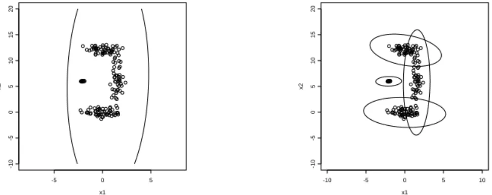
For each combination we run 100 simulations using the statistical package S-plus. Figure 1 shows one of the generated data sets for situation 6. The superimposed detection contours for two of the methods show that the outlier detection with previous clustering is much more appropriate to this situation.
x1 x2 -5 0 5 -10 -5 0 5 10 15 20 x1 x2 -10 -5 0 5 10 -10 -5 0 5 10 15 20
Fig. 1. Non-normal bivariate data with outliers and simultaneous detection contours (α = 0.1) with: single robust Mahalanobis distance using RMCD25 (left panel); mclust with k = 4 and RMCD25 (right panel).
Tables 1 and 2 give the results of the simulation in terms of “proportion of runs with correct identification of all the outliers,” p1, “average proportion of
outliers masked over the runs,” p2, “average proportion of swamping over the
runs,” p3, and “proportion of runs without swamping” (see the simulation
study of Kosinski, 1998).1A good method should have p
1= 1, p2= 0, small
p3 and p4 = 1− α = 0.9. For the normal data all the methods behave very
well, except for some masking with the classical Mahalanobis distance, which is not surprising. For nonnormal data the best performance is achieved by mclust with k = 4 and k = 5, without significant differences between the classical and the robust estimators. The failure of the k-means method is justified by the remarkable non-sphericity of the distributions chosen.
4
Examples
We have used the proposed method (with the same variants chosen for the simulation study) on the HBK data set (also analysed by several authors, like Rousseeuw and Leroy, 1985, or Rocke and Woodruff, 1996). All the variants detected exactly the 14 known outliers.
A more complicated data set was also analysed: the “pen-based automatic character recognition data” (available from http://www.ics.uci.edu/∼mlearn /MLSummary.html). We have selected one of the classes, corresponding to the digit “0” with 1143 cases on 16 variables. An interesting feature of this data is that the characters can be plotted making it easy to judge the ad-equacy of the outlier detection (which is very convenient for checking on competing methods but very tedious to do for all the observations, besides the aim is to perform automatic classification). The single Mahalanobis dis-tance with classical estimators revealed 106 outliers. The single Mahalanobis distance with RMCD25 pointed 513 observations (!!!) most of them looking quite unsuspicious. For the other options with clustering (only k-means and pam, since mclust is not adequate for data of this size) those numbers varied from 95 to 140. Very aberrant observations were detected by all the methods including classical Mahalanobis distance. However, ten strange observations (looking more like a “6” than a “0”) were detected by all the clustering meth-ods but not by the classical Mahalanobis distance. In future work we intend to assess the impact of this on the accuracy of the discrimination process for the whole data set.
5
Conclusions
From the simulation study and from the examples we conclude that the proposed method is promising. However, some refinements may be necessary. We intend to try other (more efficient) robust estimators and to perform a more extensive simulation study, namely to investigate the performance on larger data sets, higher contamination, and the instability of the indicator p4.
References
Banfield, J.D. and Raftery, A.E. (1992). Model-based Gaussian and non-Gaussian clustering. Biometrics, 49, 803-822.
Becker, C. and Gather, U. (1999). The masking breakdown point of mul-tivariate outlier identification rules. Journal of the American Statistical Association, 94, 947-955.
1For the cases without outliers p
Clust. MD with RMCD25 MD with ¯x and S Situation Method k p1 p2 p3 p4 p1 p2 p3 p4 k-means 3 nd nd 0.000 1.00 nd nd 0.002 0.78 “ 4 nd nd 0.005 0.53 nd nd 0.001 0.87 “ 5 nd nd 0.003 0.67 nd nd 0.002 0.85 Normal pam 3 nd nd 0.000 1.00 nd nd 0.002 0.78 p = 2 “ 4 nd nd 0.005 0.58 nd nd 0.002 0.78 Without “ 5 nd nd 0.004 0.65 nd nd 0.001 0.81 outliers mclust 3 nd nd 0.000 1.00 nd nd 0.001 0.93 “ 4 nd nd 0.003 0.75 nd nd 0.000 0.95 “ 5 nd nd 0.002 0.78 nd nd 0.001 0.92 none 1 nd nd 0.001 0.92 nd nd 0.001 0.91 k-means 3 1.00 0.00 0.000 1.00 1.00 0.00 0.002 0.76 “ 4 1.00 0.00 0.006 0.51 1.00 0.00 0.002 0.69 “ 5 1.00 0.00 0.004 0.62 1.00 0.00 0.001 0.85 Normal pam 3 1.00 0.00 0.000 1.00 1.00 0.00 0.002 0.73 p = 2 “ 4 1.00 0.00 0.005 0.54 1.00 0.00 0.002 0.75 With “ 5 1.00 0.00 0.003 0.66 1.00 0.00 0.002 0.75 outliers mclust 3 1.00 0.00 0.000 1.00 1.00 0.00 0.001 0.85 “ 4 1.00 0.00 0.003 0.72 1.00 0.00 0.001 0.82 “ 5 1.00 0.00 0.003 0.72 1.00 0.00 0.001 0.93 none 1 1.00 0.00 0.001 0.88 0.84 0.16 0.001 0.93 k-means 3 nd nd 0.000 1.00 nd nd 0.001 0.91 “ 4 nd nd 0.001 0.94 nd nd 0.000 0.95 “ 5 nd nd 0.000 0.99 nd nd 0.000 0.99 Normal pam 3 nd nd 0.000 1.00 nd nd 0.001 0.91 p = 4 “ 4 nd nd 0.001 0.93 nd nd 0.001 0.93 Without “ 5 nd nd 0.000 0.95 nd nd 0.000 0.99 outliers mclust 3 nd nd 0.000 1.00 nd nd 0.000 0.98 “ 4 nd nd 0.001 0.91 nd nd 0.000 1.00 “ 5 nd nd 0.001 0.94 nd nd 0.001 0.98 none 1 nd nd 0.000 0.95 nd nd 0.001 0.91 k-means 3 1.00 0.00 0.000 1.00 1.00 0.00 0.003 0.67 “ 4 1.00 0.00 0.007 0.44 1.00 0.00 0.003 0.69 “ 5 1.00 0.00 0.005 0.57 1.00 0.00 0.001 0.82 Normal pam 3 1.00 0.00 0.000 1.00 1.00 0.00 0.002 0.76 p = 4 “ 4 1.00 0.00 0.005 0.52 1.00 0.00 0.002 0.81 With “ 5 1.00 0.00 0.004 0.65 1.00 0.00 0.001 0.87 outliers mclust 3 1.00 0.00 0.000 1.00 1.00 0.00 0.002 0.80 “ 4 1.00 0.00 0.005 0.64 1.00 0.00 0.001 0.87 “ 5 0.99 0.01 0.003 0.71 1.00 0.00 0.001 0.89 none 1 1.00 0.00 0.001 0.84 0.60 0.40 0.004 0.94 Table 1. Results of the simulation study for normal data.
Becker, C. and Gather, U. (2001). The largest nonidentifiable outlier: a com-parison of multivariate simultaneous outlier identification rules. Compu-tational Statistics and Data Analysis, 36, 119-127.
Davies, P.L. and Gather, U. (1993). The identification of multiple outliers. Journal of the American Statistical Association, 88, 782-792.
Kaufman, L. and Rousseeuw, P.J. (1990). Finding Groups in Data: An In-troduction to Cluster Analysis. New York: Wiley.
Kosinski, A.S. (1998). A procedure for the detection of multivariate outliers. Computational Statistics and Data Analysis, 29, 145-161.
multi-Clust. MD with RMCD25 MD with ¯x and S Situation Method k p1 p2 p3 p4 p1 p2 p3 p4 k-means 3 nd nd 0.199 0.14 nd nd 0.063 0.60 “ 4 nd nd 0.017 0.77 nd nd 0.037 0.72 “ 5 nd nd 0.005 0.82 nd nd 0.022 0.77 Non-normal pam 3 nd nd 0.193 0.16 nd nd 0.029 0.74 p = 2 “ 4 nd nd 0.012 0.73 nd nd 0.030 0.63 Without “ 5 nd nd 0.006 0.70 nd nd 0.036 0.73 outliers mclust 3 nd nd 0.046 0.81 nd nd 0.041 0.73 “ 4 nd nd 0.018 0.71 nd nd 0.044 0.75 “ 5 nd nd 0.001 0.83 nd nd 0.024 0.84 none 1 nd nd 0.001 0.90 nd nd 0.000 0.99 k-means 3 0.94 0.06 0.213 0.06 0.14 0.86 0.035 0.81 “ 4 0.38 0.62 0.104 0.52 0.00 1.00 0.067 0.61 “ 5 0.50 0.50 0.023 0.75 0.51 0.49 0.040 0.72 Non-normal pam 3 0.89 0.11 0.207 0.11 0.18 0.82 0.046 0.73 p = 2 “ 4 0.84 0.16 0.169 0.23 0.00 1.00 0.045 0.74 With “ 5 0.83 0.17 0.008 0.72 0.53 0.47 0.045 0.71 outliers mclust 3 0.21 0.79 0.054 0.78 0.17 0.83 0.047 0.75 “ 4 0.99 0.01 0.026 0.80 0.99 0.01 0.043 0.73 “ 5 0.94 0.06 0.009 0.80 1.00 0.00 0.014 0.85 none 1 0.00 1.00 0.000 0.96 0.00 1.00 0.000 1.00 k-means 3 nd nd 0.181 0.25 nd nd 0.018 0.78 “ 4 nd nd 0.028 0.71 nd nd 0.026 0.82 “ 5 nd nd 0.008 0.85 nd nd 0.040 0.76 Non-normal pam 3 nd nd 0.124 0.47 nd nd 0.016 0.80 p = 4 “ 4 nd nd 0.007 0.82 nd nd 0.037 0.81 Without “ 5 nd nd 0.005 0.89 nd nd 0.033 0.76 outliers mclust 3 nd nd 0.034 0.86 nd nd 0.006 0.90 “ 4 nd nd 0.007 0.88 nd nd 0.012 0.85 “ 5 nd nd 0.002 0.91 nd nd 0.013 0.89 none 1 nd nd 0.001 0.90 nd nd 0.000 0.97 k-means 3 0.76 0.24 0.205 0.21 0.07 0.93 0.019 0.82 “ 4 0.13 0.87 0.045 0.57 0.01 0.99 0.074 0.75 “ 5 0.16 0.84 0.015 0.69 0.26 0.74 0.040 0.79 Non-normal pam 3 0.66 0.34 0.168 0.33 0.06 0.94 0.016 0.79 p = 4 “ 4 0.88 0.12 0.131 0.36 0.02 0.98 0.043 0.8 With “ 5 0.74 0.26 0.013 0.79 0.21 0.79 0.042 0.78 outliers mclust 3 0.23 0.77 0.291 0.53 0.18 0.82 0.171 0.64 “ 4 1.00 0.00 0.013 0.84 0.99 0.01 0.009 0.88 “ 5 0.94 0.06 0.007 0.92 0.98 0.02 0.015 0.90 none 1 0.00 1.00 0.001 0.90 0.00 1.00 0.000 0.96 Table 2. Results of the simulation study for non-normal data.
variate data. Journal of the American Statistical Association, 91, 1047-1061.
Rousseeuw, P.J. (1985). Multivariate estimation with high breakdown point. In: Mathematical Statistics and Applications, Volume B, eds. W. Gross-man, G. Pflug, I. Vincze and W. Werz 283-297. Dordrecht: Reidel. Rousseeuw, P.J. and Leroy, A.M. (1985). Robust Regression and Outlier
Detection. New York: Wiley.
Rousseeuw, P.J. and von Zomeren, B.C. (1990). Unmasking multivariate outliers and leverage points. Journal of the American Statistical Associ-ation, 85, 633-639.