The effects of the large-scale asset purchase programs launched by the ECB and the FED

(1)

1

The effects of the

Large-Scale Asset Purchase

programs launched by the

ECB and the FED

Pedro Branco Pardal

152418079

Dissertation written under the supervision of Professor Carla Soares

Dissertation submitted in partial fulfilment of requirements for the MSc in

Finance, at the Universidade Católica Portuguesa, January 2020.

(2)

2

What are the effects of the Large-Scale Asset Purchase

programs launched by the ECB and the FED?

Abstract

This Dissertation explores the effects of the large-scale asset purchase programs launched by the European Central Bank in 2014 and by the Federal Reserve in 2008 and compare the results across the two economies. We start by investigating whether the programs had effects in reducing financial market tensions by analyzing the daily behavior of some market indicators around important announcement dates. Then, by employing a standard VAR, we analyze the impact of an asset purchase shocks in main macroeconomic indicators, such as output and prices, and in financial markets indicators, such as bond yields and stock prices. From the first analysis, the results suggest that both Central Banks made announcements that had immediate effects in reducing bond yields, depreciating the domestic currency and boosting stock prices. From the VAR analysis, we conclude that the US program was more effective in rising output, inflation and stock prices than the ECB program, and that both programs were able to decrease both long term government and corporate bond yields of the respective economy. However, it was found stronger evidence for the US dollar depreciation during the US period studied than for the euro area domestic currency depreciation during the ECB program.

Keywords: Asset purchase program effects, Unconventional monetary policy, VAR, Quantitative Easing, Announcement dates

(3)

3

Quais são os efeitos dos programas de compra de activos em

grande escala lançados pelo BCE e pelo FED?

Resumo

Esta dissertação explora os efeitos dos programas de compra de activos em grande escala lançados pelo Banco Central Europeu (BCE) em 2014 e pela Reserva Federal em 2008 e compara os resultados das duas economias. Começamos por investigar se os programas tiveram efeitos em reduzir tensões nos mercados financeiros através da análise do comportamento em frequência diária de alguns indicadores de mercado, à volta de datas importantes de anúncio. Depois, através da aplicação de um standard VAR, analisamos o impacto de choques de compras de activos nos principais indicadores macroeconómicos, como o índice industrial e os preços de mercado, e em indicadores de mercados financeiros, como o rendimento de obrigações e o preço das acções. Da primeira análise, os resultados sugerem que ambos os Bancos Centrais fizeram anúncios que tiveram efeitos imediatos em reduzir o rendimento das obrigações, em depreciar a moeda doméstica e em subir o preço das acções. Da análise feita pelo VAR, conclui-se que o programa dos Estados Unidos da América (EUA) foi mais eficaz em aumentar o índice industrial, a inflação e o preço das acções do que foi o programa do BCE, e que ambos os programas tiveram sucesso em reduzir o rendimento das obrigações governamentais e corporativas da respectiva economia. Contudo, foi encontrada uma mais forte evidência da depreciação do dólar americano durante o período do programa dos EUA do que a depreciação verificada no euro durante o período do programa estudado do BCE.

(4)

4

Acknowledgements

I would like to thank my supervisor, Professor Carla Soares, for all the support, dedication and availability demonstrated during all the thesis semester. Without the comments and advices given throughout the period, I would never been able to submit the present dissertation. Thank you very much for this opportunity to work together with you.

I would also like to thank my family, for all the help and motivation given throughout my whole life, and specially my parents, João and Isabel, that have playing a huge an important role in my life and education.

Further, I would like to thank all my friends, for the support and confidence provided during this period, that helped me facing the problems that eventually occurred while working on the dissertation.

Lastly, I would like to thank the University Católica-Lisbon for having contributed towards my interest in finance, that has encouraged me into approaching this topic.

(5)

5

List of abbreviations

ABSPP – Asset-backed Securities Purchase Programme

BEIR – Break-Even Inflation-linked rate

CB – Central Bank

CBPP3 – Third Covered Bond Purchase Programme

CSPP – Corporate Sector Purchase Programme

ECB – European Central Bank

EER – Effective Exchange rate

FED – Federal Reserve

GFC – Great Financial Crisis

LSAP – Large-Scale Asset Purchase

MBS – Mortgage-Backed Security

PSPP – Public Sector Purchase Programme

QE – Quantitative Easing

TIPS – Treasury Inflation Protection Securities

US – United States

(7)

7

1. Introduction

In the wake of the Great Financial Crisis (GFC) in 2008, some of the largest central banks in the world (such as the FED and the ECB) had to intervene in the economy in order to reduce the tensions that were present around the financial markets. These tensions could dangerously jeopardize the global economy and had shaken both the European and American economies. To provide monetary stimulus and to tackle the risk of a very prolonged period of low inflation, central banks act through a variety of monetary policy measures such as lowering interest rates, which is the most common one.

The FED and the ECB have lowered interest rates to the lower-bound level, exhausting the most used instrument of monetary policy so far. In order to effectively respond to the needs that the financial crisis have caused, central banks started making large scale asset purchases (LSAP) (also known as Quantitative Easing) in order to ensure financial stability and stimulate the economy.

In the case of the ECB, the programs we are focusing in the present dissertation consist of those under Asset Purchase Programme (APP1_{), i.e. the following: corporate sector purchase} programme (CSPP), public sector purchase programme (PSPP), asset-backed securities purchase programme (ABSPP) and the third covered bond purchase programme (CBPP3). An underlying aspect of the PSPP is that it is implemented in a decentralized fashion2_{: the National} Central Banks (NCBs) are the ones responsible for purchasing 92% of the total amount, leaving the remaining 8% to the ECB. The ECB has its purchases limited to government bonds and agency securities across all eligible jurisdictions while the NCBs are restricted too, but to purchases of domestic bonds issued by the central governments or recognized agencies of their own jurisdiction up to limits consistent with the prohibition of monetary financing.

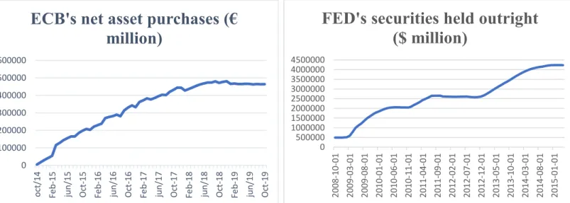
The size of the APP launched by the ECB (October 2014 to November 2019) was of about €2,673 billion and the Fed’s LSAP (March 2009 to December 2014) was around $4,500 billion. The effects in Italy of the ECB’s first rounds of asset purchase are considered to have resulted into increased investment by firms, that saw their cost of capital lowered, and increased consumption from households, that found saving was less profitable (Ferrero and Cova (2015)).

1_{https://www.ecb.europa.eu/mopo/implement/omt/html/index.en.html} 2_{https://www.ecb.europa.eu/press/pr/date/2015/html/pr150122_1.en.html}

(8)

8

Given that the results of these unconventional policy measures belong to our present, as both programs have ended not so long ago, it was found interesting to approach the topic of Central Bank asset purchases for several reasons. First, it is now possible to update the ECB dataset with a more recent data and explore the effects of the euro area APP until 2019. Also, through performing a financial and macroeconomic comparative analysis of both programs it is possible to take conclusions regarding their effectiveness including a time period when both economies were recovering from the financial crisis.

The analysis developed in this dissertation focus on the identification of an asset purchase shock and used as methodology the Vector-Autoregression (VAR), where there were made several different models with and without applying restrictions, each of them with two macroeconomic variables to evaluate the effects on output and prices and adding several other variables, such as bond yields and stock indices, to evaluate the effects on the financial markets. In addition, it was also carried a daily data analysis to test the response of some of these variables on the announcements made by the CB’s regarding the asset purchases. The main concluding remarks to bear in mind from the analysis are that the Fed’s program was far more effective to boost output and inflation levels than the ECB’s during the period studied; there is evidence of decreasing bond yields (both sovereign and corporate) resulting from a shock associated to these asset purchases for both economies; and there is evidence that these shocks have impacted the stock markets and the effective exchange rate in opposite directions for the two economies such that it has depreciated (appreciated) the American (European) domestic currency and it has a positive (negative) impact on the American (European) stock markets. Having as a research question for the present dissertation an assessment on the effects of asset purchase programs for both euro area and US economies, the analysis is structured as follows: section 1 introduces to the context where both programs took place and provides a broad picture on the policy monetary measures; section 2 offers a diversified literature review grouped into three parts: 2.1 aims to explore some of the previous main transmission mechanisms tested from which these policies are transmitted into the economy and financial markets, 2.2 offers a notion of recent methodologies used addressing to the effects of asset purchases in the financial markets and economy while 2.3 ends the section by providing some of the previous empirical findings on these effects. We then start section 3 by presenting our standard VAR model and empirical set-up used to explore the asset purchases effects along with all the data retrieved; in section 4 the findings on the effects of asset purchases on financial market tensions are shown, followed by a daily data analysis on some of the important announcements of both ECB and

(9)

9

the Fed regarding the effects those announcements had on some of the financial markets indicators also used in our VAR model. Section 5 provides the results found in the VAR analysis through an evaluation of the impulse response functions found for the set of variables tested and section 6 provides some of the important concluding remarks to bear when exploring the effects of asset purchases.

2. Literature Review

This next section aims to provide an overview of the literature on the asset purchases effects and how these are transmitted to the financial markets, reviewing also the methods followed by different studies, so that the approach and results achieved in the present dissertation can be compared and contextualized.

2.1 Main Transmission Channels

The central banks’ asset purchases are transmitted to the economy through several channels. The first category of channels that we will see in this section is the signaling channel, which is considered as one of the most influent channels of monetary policy transmission (Bauer and Rudebusch (2014)). This channel operates through the monetary authority’s commitment to its mandate and it can impact the economy and the financial markets in different ways. This channel is activated by influencing market expectations regarding future short-term interest rates as the long-term maturity assets purchased by the CB’s lead to a long period of higher liquidity. The perceived commitment of the central bank can also anchor or boost inflation expectations. The result of higher inflation expectations will be lower real long-term interest rates, that will ultimately increase investment and consumption. To sum up, we could say that this channel when activated signals to the financial markets that an expansionary asset purchase program makes interest rates remaining at a lower level for a longer period showing commitment of the monetary authority to maintain its price stability objective.

Another transmission channels through which these massive purchases are expected to work is the portfolio rebalancing channel. This channel is based on the creation of incentives for institutions to rebalance their portfolios into, in particular, riskier assets, benefiting agents through lower costs of borrowing. The channel relies on the assumption that agents have a

(10)

10

preferred habitat, i.e. investors prefer, for instance, a given maturity in the bond market causing imperfect substitutability between assets (Vayanos and Villa, 2009). If bonds and central bank reserves were perfect substitutes, the purchases would have no effect (Joyce et al., 2012). There is evidence suggesting that the portfolio rebalancing channel was activated and transmitted to the financial markets during the asset purchase programs of economies where LSAPs where made, represented by the decreasing yields of both assets purchased and not purchased during the program (United States evidence see Gagnon et el. 2011, for the UK see Joyce et al. 2014). Andrade et al. (2016) states that the asset valuation channel (also called portfolio rebalancing channel through the notion that a variation in asset prices will cause a change in the investors’ optimal share of those assets) can be activated through two ways. First, it suggests that an increase in the average duration of the government bonds purchased would lead to a decrease in the duration risk from the private sector, as longer maturities bonds would belong to the Central Banks’s balance sheet. The second relies on the assumption that the spread of those government bonds is related to the investors’ leverage constraints or risk bearing capacity as mentioned by Vayanos and Villa (2009). An example could be that this constraint is present when investors face value-at-risk constraint (Adrian and Shin, 2014) given that a central bank large asset purchase will reduce the price of the market risk and hence, inducing a relaxation in the risk constraint.

Besides the portfolio rebalancing, there are other indirect effects that are triggered through changes on interest rates. The fact that there is more domestic currency circulating in an economy, it will depreciate it in relation to other currencies, activating the called exchange rate channel. Gambetti and Musso (2017) found evidence on the activation of this channel during the ECB program and have the opinion that this channel can be seen as a particular category within the portfolio rebalancing channel as domestic residents may increase its demand for external assets.

Some macroeconomic effects around QE have been studied and there is evidence that it can indeed stimulate the economy through these channels. Furthermore, most authors that research on APP support that the portfolio rebalancing channel is amongst the most influent channels in monetary policy transmission to the financial markets (Altavilla et al. (2016) for the euro area and Gagnon et al. (2011) for the US).

In the present dissertation we assess the portfolio rebalancing channel through the impact on the bond (both sovereign and corporate segments) and equity markets and the exchange rate

(11)

11

channel through the evaluation of the variations in the effective exchange rate during the LSAPs.

2.2 Different methodologies accessing the effects of LSAPs

To assess the effects in the economy and in the financial markets of these unconventional monetary policies, several methodologies can be applied.

Event study methodologies are also widely used approaches to study monetary policy transmission, being worth mentioning Joyce et al. (2011) and Dell’Ariccia et al. (2018). Joyce el al. (2011) addresses to the risk of performing an event study analysis considering an inappropriate window length. In their results on the UK economy, it is highlighted that choosing a one-day over a two-day window have considerably halved the results. In light of such possible misapplications, it was decided in the present dissertation not to carry out solely with an event study analysis to assess the asset purchases effects in the economy and in the financial markets. Gambetti and Musso (2017) brought a model that allows for important changes in the economy, such as periods ranging from the GFC to a transition where interest rates are at the ZLB, allowing the model to be flexible in these terms. Their approach is a time-varying VAR with stochastic volatility that seems to be appropriate given the uncertainty lived in the economic behavior and in monetary policy rules, but the high computational costs inherited to the model assumes an important factor to consider when choosing the approach. Considering the advantages and disadvantages of this approach, it seemed reasonable not to follow it in the present dissertation given the relatively short time frame captured in our analysis (5 to 6 years) that doesn’t require such computational costs to capture major structural changes in the economy or volatility.

A different methodology is explored by Beck, Duca and Stracca (2019) to study the causal effect of QE policies on financial outcome variables. They apply an augmented inverse probability weighting (AIPW) estimator that addresses potential endogeneity by re-randomising the sample using propensity score estimators. They perform the study by applying local projections to the re-randomised sample so that they can evaluate the treatment and side effects. The lack of familiarity with this approach and the large number of observations that is needed to apply this methodology led me to follow other, more suitable options.

(12)

12

Gambacorta et. al (2014) studies the effectiveness of unconventional monetary policies by exploring the cross-sectional dimension of eight economies (Canada, the euro area, Japan, Norway, Sweden, Switzerland, the United Kingdom, and the United States) at a time where economies were at the ZLB. The cross-sectional dimension is done through a panel VAR which makes sense given the high number of economies. This methodology makes it possible to test whether there is correlation across the residuals among the different economies while monetary policy shocks can be simultaneously identified, allowing also to consider the differences in the transmission mechanisms of monetary policy across the economies. Given that the present dissertation is only focusing in two economies, in two different time frames, it makes little sense to adopt this method in our analysis.

The approach followed in the present dissertation was influenced on the work of the previous author, but it gives also special relevance on the work of Weale and Wieladek (2016). There are three main underlying differences: they analyze two economies that are launching LSAP within the same time frame (USA and UK), they have a combination of sign and time restrictions for their four identification schemes tested, and lastly, they employ a Bayesian VAR approach developed by Uhlig (2005) and Peersman (2005).

Considering the different methodologies approached to study unconventional monetary policy, the present dissertation employs a standard VAR with a lag of 2 (two) as it was found and used by these previously mentioned authors to be the appropriate value for the analysis considered. We then proceed to the evaluation of the results by looking at the impulse response functions in our different set ups considered and that will be carefully detailed further in this paper.

2.3 Empirical findings on LSAPs and its effectiveness

There are several studies with empirical evidence on the results of LSAPs and its advantages and disadvantages. Overall, a continuous rise in asset prices is expected and this effect is larger on the presence of financial distressed conditions (Krishnamurthy and Vissing-Jorgensen (2013)). Most authors agree that an expansionary asset purchase program contributes to a decrease in the financial market tensions such as the presence of highly volatile markets and financial distressed conditions.

Dell’Ariccia et al. (2018) focused on unconventional monetary policies in countries such as the UK, Japan and Euro area, reaching to some important conclusions, in particular the increased

(13)

13

effectiveness during financial distress and the convincing significant impact of the policies in both financial conditions and macro variables. The effectiveness is measured through inflation, policy rates, GDP and central bank assets in order to assess the capacity demonstrated during the period studied in preventing further financial distress, restoring the normal functioning of the financial markets, and providing additional monetary stimulus by lowering long-term interest rates. The above conclusions reached are based on government borrowing costs and policy rates evolution across different countries and relating that evolution with the observed levels of output, long-term government yields and prices.

Beck et al. (2019) findings are in line with the previous authors on an important and motivating evidence that these nonstandard policies bring no major side effects and increases in risk. Through a cross country analysis with a panel data of 41 countries, they reach to two important conclusions that QE (1) did not increase or fall significatively real house prices and real credit to the private sector and (2) there is no evidence of particularly large shifts in capital flows. These conclusions appear to be in favor of unconventional monetary policies and thus a better understanding of its effectiveness and impact is highly desirable to all economic agents. There is empirical evidence supporting that QE contributed to boost the economy and ease monetary conditions through lower bond yields, credit risk spreads and interbank rates as specified in Borio and Zabai (2016) with an analysis of the European, American, English and Japanese economies.

In the UK, the purchase of long-term government bonds through the LSAP encouraged institutional investors into replacing holdings of government bonds by corporate bonds, thus decreasing the yields on both securities. Evidence for the US (Gagnon et al. (2011)) and for the UK (Joyce et al. 2014) shows that the effect of LSAP not only affected long term treasury securities but also corporate bond yields, by about the same amount. One could infer that this low tradeoff between both public and private sector assets is given by the lower credit risk premiums and improved economic prospects that the asset purchases bring to the economy. Altavilla et al (2016) show that long term government bond yields have decreased significantly by evaluating ECB’s January 2015 announcement, at a time when the degree of financial market stress was relatively low. The authors highlight that the strength of the channels of transmission might differ across liquidity and risk regimes as investor’s effectiveness to integrate across different segments in the market as QE takes place, is related with its risk bearing capacity. We have already seen that unconventional monetary measures have a substantial impact of

(14)

14

increasing asset prices in the presence of high financial distress (Dell’Ariccia et al. (2018)) through portfolio rebalancing channel, but these authors concluded that during periods of low distress (2015), the weak local supply channel has facilitated spill-overs to non-targeted assets such as corporate bonds.

Haldane et al. (2016) explores the effects of asset purchase shocks and relate the shock with the state of the financial markets, for the US and UK over the same period. They follow a similar VAR approach as the one employed in this dissertation (Weale and Wieladek (2016)) concluding that the effects of the shocks are larger in periods when market stress is high and smaller when it is low. The results are achieved using a sub-sample analysis comparing the shock effects captured in 2007-2010 with the ones captured from 2010 onwards, when market stress is lower.

The results achieved by the authors that have employed similar or different approaches on VAR models (Weale and Wieladek (2016), Hesse, Hofmann and Weber (2017), Gambetti and Musso (2017)) lead all to similar results. They conclude that an asset purchase shock lead to a small but persistent increase in output and on prices.

Ferrero and Cova (2015) come to interesting conclusions when stating that the impact of the APP on prices comes directly from the exchange rate channel. The results are due to the greater competitiveness on prices and acceleration in economic activity attributable to the depreciation of the euro.

The US asset purchase program differs from the ECB’s in some respects such as the asset class purchased and time frame for example. But when considering the MBS (mortgage-backed securities)3_{program that only had place in the US, studies demonstrate that the LSAP’s had} impact through other channels like scarcity and capital constraints channel (Krishnamurthy and Vissing-Jorgensen (2013)).

It is also seen in this paper that effects on long term rates will affect asset prices such as stocks or exchange rates, to the extent that these represent the expected discounted stream of future cash flow and so, a change in these rates will generate a new price equilibrium. This increase

3_{MBS are different from government or corporate bonds as these are subject to “prepayment risk” (Bhattarai and}

Neely (2016)) meaning that the mortgage holders can prepay their mortgage without penalty. This feature works just like a call option: the holder will call the option if long interest rates decline below the yield on the MBS as it will be cheaper for the holder to refinance.

(15)

15

in bond prices (decrease in yields) and in asset prices is quite often mentioned in literature as a natural consequence of QE.

3. Data and Empirical set-up

To perform the analysis, it was followed the standard Vector Auto-Regression (VAR) approach with a lag4_{of two months to access the effects of asset purchases in the Euro area and in the} United States throughout the period of October 2014 to September 2019 and October 2008 to December 2014, respectively. The window length chosen for this analysis was based on the initial and end periods of unconventional monetary policy measures adopted by the respective Central Banks (ECB and FED) as shown in figure 1 and figure 2, represented in the ECB’s and Fed’s increase in balance sheets assets.

Figure 1 - purchases for the ECB under the programs PSPP, CSPP, ABSPP and CBPP3. Source ECB website

4_{Lags of 6 and 4 were also considered for robustness check, but the results were not significatively different from}

the ones found using 2 lags. Results of the model with different lags can be found in the appendix.

0 100000 200000 300000 400000 500000 600000 o ct/14 Fe b -15 ju n /15 O ct -15 Fe b -16 ju n /16 O ct -16 Fe b -17 ju n /17 O ct -17 Fe b -18 ju n /18 O ct -18 Fe b -19 ju n /19 O ct -19

ECB's net asset purchases (€

million)

0 500000 1000000 1500000 2000000 2500000 3000000 3500000 4000000 4500000 2008-10-01 2009-03-01 2009-08-01 2010-01-01 2010-06-01 2010-11-01 2011-04-01 2011-09-01 2012-02-01 2012-07-01 2012-12-01 2013-05-01 2013-10-01 2014-03-01 2014-08-01 2015-01-01

FED's securities held outright

($ million)

Figure 2 - cumulative result of permanent open market operations. Source FRED website

(16)

16

Below in figure 3 we can find the relative size of the ECB’s and the FED’s balance sheet assets relative to its GDP in its respective local currency (€ and $).

Figure 3 – Ratio of Assets/GDP for the euro area and USA. Source ECB: ECB SDW and Eurostat. Source Fed: FRED website

Note: for the ECB, we considered as assets the sum of two Eurosystem’s series: the securities of euro area residents denominated in euro plus the series that represent lending to euro area credit institutions related to monetary policies. For the Fed, we considered as assets the series Total Assets (less eliminations from consolidation). Black marks represent the implementation (by phases the USA case) of the program studied in the analysis.

To shed some light regarding the magnitude of previous LSAPs in different economies, it is known that the size of the Fed’s balance sheet assets in relation to US Nominal Gross Domestic Product (GDP) has been increasing periodically since 2008 as it is seen in the graph. Moreover, as a reflection of the unconventional policy measures taken to provide liquidity and ensure financial and macroeconomic stability, the ECB since 2010 has undertaken programs such as the Securities Market Program (SMP) and two covered bond purchase programs (CBPP1 and CBPP2). The last of these programs to be undertaken was CBPP2 that ended by the end of 2012, when the Eurosystem’s policy assets reached about 75% of GDP. The focus in the present analysis will be on the APP (as it was already mentioned), and therefore it is excluded the period when the ECB launched the just mentioned programs, in order not to bias the results concerning the APP solely, that only started in October 2014 (ECB’s graph black mark) and taking the form of monthly purchases. Since this date, we can see a large increase in the ratio from 40% to around 120% at end of the period studied. During the period studied, the ECB conducted four different programs under the APP in which there were purchased different types of

QE1 QE2 QE3 0 0.2 0.4 0.6 0.8 1 1.2 1.4 2008-10-01 2009-06-01 2010-02-01 2010-10-01 2011 -06 -01 20 12 -02 -01 20 12 -10 -01 20 13 -06 -01 20 14 -02 -01 2014-10-01 2015-06-01 2016-02-01 2016-10-01 2017-06-01 2018-02-01 2018-10-01 2019-06-01

ECB: Assets/GDP

QE1 QE2 + MEP

QE3 QE1 QE2 + MEP

QE3 0 0.05 0.1 0.15 0.2 0.25 0.3 2008-10-01 2009-03-01 2009-08-01 2010-01-01 2010 -06 -01 2010-11-01 2011-04-01 2011-09-01 2012-02-01 2012-07-01 2012-12-01 2013-05-01 2013-10-01 2014-03-01 2014-08-01 2015 -01 -01

FED: Assets/GDP

QE1 QE2 + MEP

(17)

17

securities. During the CSPP, ABSPP and CBPP3 the ECB bought respectively, corporate sector bonds, asset-backed securities and covered bonds while during the PSPP, the purchases include nominal and inflation-linked central government bonds and bonds issued by recognized agencies, regional and local governments, international organizations and multilateral development banks located in the euro area.

In the case of the FED, the programs considered can be distinguished into four phases: QE1, QE2, MEP (maturity extension program) and QE3. The Q1 and MEP involved purchases of mortgage-backed securities (MBS), agency debt and Treasury securities while the other two programs focused on singularly purchasing one type of these assets at a time: QE2 focused only on purchases of Treasuries and QE3 only on MBS. The first black mark in the Fed’s graph correspond to the beginning of QE1 (November 2008), that is followed in March 2009 by which is considered to be one of the most important but economically harsh announcements as the Fed declared that would purchase additional assets ($1,150 billion) beyond the purchases already announced by the end of 2008, reflecting poor economic prospects. The second mark corresponds to the beginning of QE2 at the end of 2010. The last mark shown in the graph corresponds to the beginning of QE3 in September 2012 when the Fed stated that the goal set was to purchase $40 billion of MBS per month as long as “the outlook for the labor market does not improve substantially… in the context of price stability”.

As mentioned, the analysis is based on a VAR that takes the form: • Yt = α + A(L)Yt-1 + Bεt

where Yt is a vector of endogenous variables, α is a vector of constants, A(L) a matrix polynomial in the lag operator L, and B is the contemporaneous impact matrix of the mutually uncorrelated shocks εt. The variables present in the model are all in monthly frequency, but some of them differ across the two economies as the proxys considered are different.

For the ECB case, it was considered the logarithm of Industrial Production Index (Indprod) as a measure of output; the measure of prices is the logarithm of Harmonized Index of Consumer Prices (HICP) excluding food and energy (in order to diminish the exogenous impact of oil price shocks); the IBOXX Break-even inflation-linked (BEIR) yield, the 10-year AAA and All (issuers and ratings) government bond yields for the euro area and the IBOXX euro corporates bond yield measure the reaction in the bond markets; the logarithm of real effective exchange

(18)

18

rate (REER) to measure domestic currency depreciation; the logarithm of the EUROSTOXX600 Index as Stock Prices and the cumulative APP series to measure the shock. Three IBOXX bond indices were used, for both European and American corporate bond yields and for the inflation-linked yield (BEIR) as they offer good benchmarking, regular market segment reviews and transparency. The euro IBOXX indices are market-value-weighted and are based on real-time prices while the US IBOXX indices are volume-weighted and are based on US end of day prices. All the IBOXX indices are calculated on the last calendar day of each month irrespective of holidays and weekends.

The two 10-year maturity government bond yields that were used in the estimation of the VAR model are taken from the yield curve spot rate, continuous compounding, yield error minimization, provided by the ECB. The underlying difference between these two yields is the group of issuers, where in one are considered all euro area issuers independently of the rating and in the other only AAA-rated issuers are included. Variables were used in real terms. The EER and BEIR are already in real terms, the yields and the stock prices were deflated with the HICP.

For the USA, it was considered the logarithm of Industrial Production Index (Indprod) as a measure of output; the logarithm of personal consumption expenditures as prices (PCE) as the measure for prices; the 10-year Government bond yield, the 10-year Treasury inflation-indexed Securities (TIPS) and the IBOXX USD corporates bond yield to measure the reaction in the bond markets; the logarithm of Trade Weighted US Dollar Index to measure domestic currency depreciation; the logarithm of the S&P500 Index as stock prices and the Securities held outright in the Federal Reserve balance sheet to measure the asset purchase shock. The choice to use the PCE as prices is justified by being the reference measure used by the Fed to assess its inflation objective, and it offers a wider group of expenses than the Consumer Price Index (CPI) such as employer related health care expenses. Variables were also used in real terms. The TIPS were already in real terms but the bond yields, the exchange rate and the stock prices were deflated with the PCE.

To have comparable results across the two economies, we also compute the ratio of the cumulative asset purchase series over the 2015Q1 value of GDP (value of first quarter of 2015 nominal Gross Domestic product) for the ECB and 2009Q1 value of GDP for the Fed, to measure the asset purchase impulse response. The results observed under this view should be seen as the impact in each of the variables (output, prices, bond yields, exchange rate, stock

(19)

19

prices and asset purchases) after an asset purchase shock that is equal to 1% of the nominal GDP in the respective quarter.

The sources used for the variables retrieved can be seen in the appendix.

4. Empirical analysis of the LSAPs

4.1 Empirical evidence of impact on financial market tensions

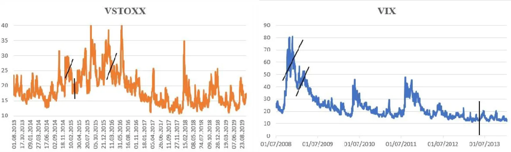
There are several ways to identify how an economy is reacting to certain policy measures and to take conclusions regarding its possibilities of overcoming from economic recession. In order to analyze how are the financial markets’ reactions to news, one could look at the volatility indexes, as the VSTOXX and the VIX (for a more detailed discussion of the VIX and its interpretation, see Whaley (2009)). VIX and VSTOXX are measures of implied volatility in the S&P500 and Eurostoxx50 indices options, respectively. Thus, they are a measure of future uncertainty regarding the underlying asset prices, in this case, the stock indices. Taking this into account, it is seen that there is a tendency for the volatility associated with the stock markets (both European and American economies) to decrease during the period when the APP and the Federal Reserve’s QE programs took place (figures 4, 5 and 6).

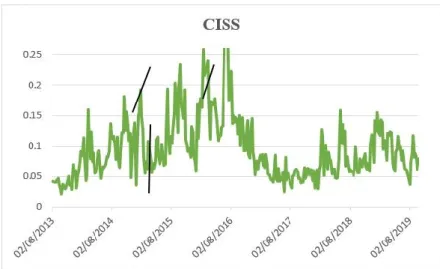
Note: For the VSTOXX and CISS graphs, we considered a time frame from 2013 to 2019 to evaluate the effects in the 22/01/2015, 09/03/2015 and 10/03/2016 ECB’s announcements. For the VIX graph we considered a time frame from 2008 to 2014 to evaluate the effects of the 25/11/2008, 18/03/2009 and 22/05/2012 Fed’s announcements. Black marks represent the value of each indicator at each announcement date.

(20)

20

In the above three graphs, there are black lines that mark some of the important announcements that were made by the ECB (for fig4 and fig6) and by the Fed (for fig5) in order to easily explore the movements in these indicators around the announcement dates. For the ECB, we look at variations around 22 January 2015 (announcement on implementation of the PSPP), 9 March 2015 (implementation of the PSPP) and 10 March 2016 (announcement on implementation of the CSPP). For the Fed, we look to variations around 25 November 2008 (first announcement of purchases), 18 March 2009 (announcement of additional purchasing volume) and 22 May 2013 (announcement of decreasing purchasing volume).

Across the three indicators, there was a similarity found in the way their movements occurred after the first announcement dates considered (ECB’s 22 January 2015 and the Fed’s 25 November 2008): whether it was the ECB’s or Fed’s first announcement of asset purchases, there was a decrease common among the three indicators (VSTOXX, VIX and CISS) after that first announcement date.

It is noticeable that the decrease in volatility associated with the American stock markets is more acute, but it is arguable whether this so clear decrease was emphasized by the extremely high markets tensions that were predominant by the end of the year of 2008, around the time when the investment bank Lehman Brother’s bankruptcy took place, shaking the global economy.

Financial markets volatility can have contagion effects across markets and have systemic consequences to the overall economy. If we look at the Composite Indicator of Systemic Stress (CISS) for the euro area (fig6), that captures more broadly financial stress in the euro area, we can see that for the period when the ECB’s APP took place, the CISS decreased substantially. Although the effect is not immediate, it is a normal reaction given the instability present in the

(21)

21

stock markets, that non-conventional policies have a moderate effect over systemic stress conditions in the short-term.

4.2 Immediate impact of announcements on financial markets

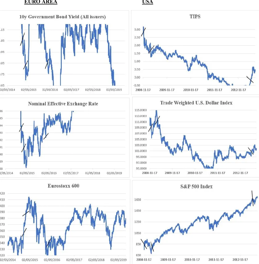
In the following section, we take a look closer to some of the financial markets variables analyzed (10y government bond yield and effective exchange rate for both economies) and assess the variations these had around the dates when important announcements regarding disclosure and implementation of the APP took place. It was also taken a greater look at the first two important announcement dates from the Fed as there were found some interesting direct effects in some variables. To do this, we used daily data on the variables to account for daily changes and there were considered the important announcement dates just mentioned in the previous section (4.1).

For the period considered, the evolution found in the variables are described in graphs below (figure 7 and 8) and the correspondent table with the values around the announcement dates can be found in the appendix 1 and 2.

By looking at the daily variations across the euro area variables, it is seen that around the first announcement date (22/01/2015), the EER and the bond yield see an immediate decrease that persists in the following days, while the eurostoxx600 index sees an increase. The 2-day and 1-week variation for the EER are -1.94% and -1.25%, respectively for the first announcement while for the second announcement, these two variations increase to the same value of -2%. Regarding the government bond yield, it is seen a strong decrease for the same 2-day and 1-week variation for the first two announcements considered (around the -14 and -16 basis points). For the eurostoxx600 index we see a stronger increase for the same two variations (2-day variation of 3.98% and 1-week variation of 2.4%) but only verified for the first announcement date. As said, the same negative effect is present in the two decreasing variables (EER and bond yield) which strengthens the already seen in literature arguments of asset purchases having the effects of decreasing bond yields and depreciating the domestic currency (Gambetti and Musso (2017)). With the 2016 announcement, the effect observed comes to be less strong and in opposite direction for these two variables, while it pushes up the stock markets index but with less intensity.

(22)

22

After the day of the first ECB announcement considered, it is possible to verify that these two variables have a decreasing trend at least until the next announcement (9 March 2015), date when the PSPP was implemented: the Government bond yield fell from 1.09 to 0.83 and the effective exchange rate fell from 93.96 to 90.15. Following the implementation, the bond yield starts rising as a presumable consequence of the markets reacting to the asset purchases, but the exchange rate continues at low stable levels, seeing a slow but positive increase. Later, when the CSPP is announced in the beginning of 2016, the yield sees a downward trend the following 6 months while the exchange rate maintains its relatively stable but increasing level, probably reflecting the continuing commitment of the ECB on keeping a loose monetary policy stance. Of course, many other factors besides policy decisions and implementation were relevant drivers of asset prices during the period considered.

The daily variations observed in the US variables for the first announcement considered (25/11/2008) are stronger for the bond and stock markets. The TIPS see an immediate and persistent decrease until the end of the month, having a strong variation in the day of the announcement of -32 b.p, -51 b.p for the 2-day variation and -113 b.p. for the 1-week variation, while stock prices also see relevant effects but in the opposite direction. As said, in the first announcement, the stock prices see a strong increase of 4.2% in the 2-day variation but in the second announcement, it is in the 1-week variation that is seen the strongest variation (4.86%). The second announcement also impacts the EER, but the effects are less strong that in the yield and stock prices. The EER sees a decrease of -1.86% and of -1.24% for the 2-day and 1-week variation. Around the last announcement considered, there were no considerably significant movements on the variables studied.

In the Fed’s program, there is a clear decrease in the TIPS yield upon the first two announcements studied. The TIPS yield mark 2.79% dated at the first announcement date, since then it decreases to 1.90% marked the day before the second announcement. On the next day (18 March 2009), the Fed announces additional purchasing volume and this yield decreases significantly to 1.28% suggesting a direct relationship between the announcements and the yield movements. The exchange rate does not see such a direct effect upon the first announcement, it steadily grows at the announcement day and it only starts decreasing after two weeks, but there is a noticeable effect on this variable on the second announcement day. Moreover, since this announcement that the variable sees a persistent decreasing trend lasting for the following years, although other factors most likely play more relevant roles.

(23)

23 EURO AREA USA

Figure 8 – Daily frequency data on some variables employed in VAR model (YIELD, EXCH and STOCKS) | Source euro area: ECB SDW and Thomson Reuters Eikon | Source USA: Fred website and Thomson Reuters Eikon

Note: the loss of information shown in the graph is due to the approximation made in the vertical axis that was found to be useful for a more detailed look at the movements around the announcement dates

(24)

24

5. Results of the VAR analysis

5.1 Identification of asset purchase shocks

The endogenous variables used in our model reflect the notion that the variables are sticky in the short run, meaning that output and prices feel no immediate effect after the impact of a monetary policy shock. The shock identified in the present dissertation is reflected through the variable “appseries” and “ratio” which represents the consecutive cumulative (monthly) rounds of asset purchase done by the ECB/FED and the ratio of this value by the respective GDP quarter valued at the beginning of each of programmes (Hesse, Hofmann and Weber (2017)). The impulse response associated with the variable “ratio” to the remaining variables present in the model will give the responses following an asset purchase shock that is equal to 1% of the respective GDP.

The assumption that the impact on output and prices is not immediate is commonly used in monetary policy transmission literature and was first presented by Christiano et al. (1996, 1999). It is possible to justify this choice for two main reasons: first, output will only see a strong and persistent impulse response if prices are sticky for a long time (Klaeffing 2003); secondly, this assumption is seen by many authors as offering a convenient way to disentangle the asset purchase shock from aggregate demand and supply shocks (Weale and Wieladek (2016)).

We apply restrictions in the model, to represent the aforementioned effect that prices and output are sticky in the short run and therefore, will not be affected upon impact but through lagged effects. This is done by employing zero-restrictions in the first two macroeconomic variables in the model (Output and Prices) so that the shock on these variables is not mixed with aggregate demand and supply shocks. It is also carried an analysis without imposing any restrictions to find out whether the differences are significantly informative or not.

Weale and Wieladek (2016) explore the macroeconomic impact of asset purchases through four different identification schemes, which allows for the identification of an asset purchase shock in different perspectives. We base our identification scheme in the first scheme presented in this paper, which applies solely zero-restrictions in some variables with the objective of representing the above described effect of price stickiness. The remaining three identification schemes adopted in the paper are explored through imposing sign restrictions, a mixture of sign and zero restrictions, and lastly, they impose sign variance decomposition restrictions.

(25)

25

This section aims to present the several results achieved through the application of the VAR model in both European and American economies. A more detailed look was given to the effect on the variation in some of the endogenous variables.

In the ECB case, it was performed a sensitivity analysis on the effect of the APP shock on 10-year government bond market relatively to the rating of the euro area countries. This is done by looking at the impulse responses of two different VAR models, where in one the variable tested is the yield on only AAA-issuers governments, while in the other model, we replace the variable by the yield on all issuers, independently of their rating.

Since the euro area represents a large group of 19 countries, that was hit by the sovereign debt crisis just before the start of the APP and was still suffering from the effects of market fragmentation, it made sense to make this distinction to account for differences in the financial markets reactions to the APP when looking separately to high rating countries (such as Germany or the Netherlands) or to all of them as a group. It is also made a third analysis of the bond markets by employing the VAR with the euro inflation-linked yield in order to confirm the results with a different measure of real bond yields.

Several models5_{were estimated, in which some were computed using the euro area data and} others using the American. The remaining differences in the models are related to small variations in some of the variables used to account for possible information related with the change, the unit in which the asset purchase shock is identified, the time horizon and we have also run the model with and without the already mentioned 0 restrictions.

5.2 Results without restrictions (asset purchase shock equal to 1% of GDP

level)

6

The results on output and prices for the euro area are broadly in line with previous results on asset purchases effectiveness, such as Weale and Wieladek (2016), Hesse, Hofmann and Weber (2017), Gambetti and Musso (2017)), meaning that they see persistent and positive increases as a result of an asset purchase shock. However, we see the results for the USA to be larger than

5_{Results found using a longer time horizon can be found in the appendix}

6_{The results from Eviews10 show the median responses within the 95% confidence intervals. Measuring the shock}

equal to one Cholesky standard deviation is also a common way to analyze the effects of unconventional monetary policy when employing a standard VAR (Behrendt (2013)). The results under this view can be found in the appendix.

(26)

26

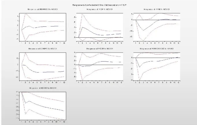
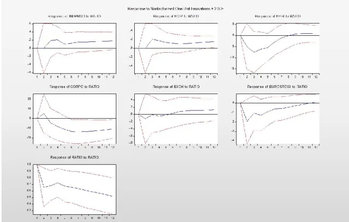
in the euro area and larger than what is usually found in the literature. Regarding output results in the euro area (figures 9, 10 and 11)7_{, following a 1% of GDP shock in asset purchases, it is} seen a peak impact of 0.18% 3 months after, although not significant, and steadily increases until 0.2%, suggesting a permanent effect of output from the APP. Prices rise following the APP start with peak at 0.41% and continuing at positive values, suggesting also a permanent effect of close to 0.2%. In the USA (figures 12 and 13), output saw a short-lived negative immediate impulse of -0.5%, probably reflecting the delayed response of output to the shock, but from month 2 onwards it rises with a peak of 1.5% from month 10 onwards. Prices see a persistent increase at about 0.9% from month 8 onwards. Based on the results achieved using the same lag length (2) but with a longer time horizon (2 years), we conclude that both effects on output and prices seem to be persistent and significant one year after the asset purchases shock. The same conclusion cannot be taken from the remaining variables present in the VAR, whose effects seem to go towards 0 after 1 year.

Relatively to the shock effects on the bond markets for the euro area, the APP seems to have induced a fall in long-term bond yields in real terms, irrespectively of the measure of yields used. The impulse responses using the BEIR (figure 9) are only slightly different from those when using the AAA (figure 10) or all issuers (figure 11) 10-year government bond yield. In the specification with the BEIR, it is seen a short-lived peak impact of -9.4bp at month 2 and increasing towards 0 afterwards, while in the specification with the deflated bond yields the impact is stronger, significant and it seems to be permanent at around -15bp. When changing the variable representing the 10-year government bond yield, whether it is a top-rated issuer or not, the results found were basically the same, meaning that the asset purchase shock had a similar impact across different sovereign issuers.

(27)

27

Figure 9 – Euro area model using BEIR (1y time horizon) | Eviews10

(28)

28

Figure 11 – Euro area model using all ratings issuers bond yield (1y time horizon) | Eviews10

About the effects in the US bond markets, it is seen that the impact of the shock is larger than in the euro area and different in the first periods. The VAR results suggest an immediate increase in yields, contrary to what could be anticipated, that vanes out through time. When using the TIPS in the model (figure 12), the effect is null at the end of the horizon, while the effect is negative and significant when using the deflated 10-year government bond yield (-140bp).

The results on bond markets are in favor of the portfolio rebalancing channel and they are complemented by the additional analysis on the corporate bond markets. The results are again quite stronger on the USA than in the euro area. The European corporate bond yields see a similar impulse reaction across all unrestricted models (figures 9, 10 and 11) of about -12bp, persistent and significant over most of the 12-month horizon and in a similar path to the government bond yields. the impact on American corporates bond yields is also similar to the impact on government bond yields, with a strong and significant decrease one year after the shock, maintaining at -190 bp after period 8 (figures 12 and 13). It is noticeable that when the model is executed with the American 10-year government instead of the TIPS, the corporate bond yield reaction is less strong (-118bp) probably related to the weaker transmission to

(29)

29

Treasury yields. Overall, the results suggest a contagion of the impact in the sovereign bond market, the one where central bank purchases were made, to the corporate bond market in similar magnitudes.

The other channel of transmission tested is the exchange rate channel, through which a depreciation of the domestic currency is expected by measures of an expansionary unconventional monetary policy, similarly to interest rate policy. There is little evidence on the activation of this channel in the euro area, as opposed to Gambetti and Musso (2017): the effective exchange has a similar behavior across all unrestricted models (figures 9, 10 and 11): there is a negative short-lived impulse (-0.2%) in the first 4 periods, but not significant, but then the euro appreciates slightly up to 0.2% in the following periods. Evidence on the American effective exchange rate depreciation is clearer in the months after the shock, with a larger magnitude than in the euro area, but it fades away over time and is not statistically significant (figures 12 and 13).

In line with the portfolio rebalancing theory, it should be expected an appreciation of equity markets. Recent literature on empirical analysis of QE indeed shows that adopting unconventional policy measures have persistent positive effects in stock markets. The VAR results do not support this hypothesis for the euro area, as European stock markets had a non-significant negative short-lived peak impact of around -1.7% (figure 9) reached during the initial phase of the program, and that it stabilized towards 0 afterwards. In contrast, for the USA we found a persistent increase in stock prices during the first 3 to 4 periods at 12% (figure 12) and 8.6% (figure 13).

One of the reasons behind these results could be that as a consequence of eased borrowing conditions, there was a greater misallocation of resources into less profitable projects8_{. The} European stock markets had a major boost at the first quarter of 2015 (initial phase of the APP) but since then, no significant growth was made, leading to the conclusion that the effect in growth beyond a short-lived boost to stocks is little.

(30)

30

Figure 12 – USA model using TIPS (1y time horizon) | Eviews10

(31)

31

By applying zero-restrictions upon impact on the first two macro variables – output and prices – we are guaranteeing that the effect felt on these variables is not immediate but is reflected through the lag order of two. With this, we achieve to similar results (figures 14 and 15) across almost all variables but with less pronounced increases on prices in both economies. The increase is roughly cut at half: in the euro area the peak is at 0.2% while for the USA the peak is at 0.7%. We can compare these values to the 0.4% and to the 1.5% concluded by the model without imposing any restrictions. It was also noticed that for the American economy, output had not the initial short-lived negative impulse felt in the unrestricted. As a result of the 0 restrictions applied, this negative short-lived impulse disappears.

Figure 14 – Euro area model applying 0 restrictions on Indprod and HICP in lag 1 and using BEIR (1y time horizon) | Eviews10

(32)

32

Figure 15 – USA model applying 0 restrictions on Indprod and HICP in lag 1 and using TIPS (1y time horizon) | Eviews10

(33)

33

6. Conclusions

The aim of the present dissertation is to evaluate the effects of the QE programs that took place in the euro area (between 2014 and 2019) and in the US (between 2008 and 2014). This form of unconventional monetary policy has been increasingly applied by several monetary authorities and a thorough look into the effects in both macroeconomic indicators and financial markets can bring insight on the effectiveness of such programs. Furthermore, through performing a comparative analysis between two major central banks as the ECB and the FED, we can take conclusions on the relationship between monetary policy decisions (such as announcements) and financial markets indicators (such as bond yields, exchange rates and stock prices).

We have seen several transmission channels that can be activated when asset purchase programs are taking place and took some conclusions that were in line with recent literature and others that were not. An evaluation on the portfolio rebalancing channel and of the exchange rate channel was made on both economies: for the euro area and US, there is evidence of portfolio rebalancing channel but there is only evidence of the activation of the exchange rate channel in the US. Portfolio rebalancing channel activation is demonstrated through the lower bond yields that were observed in both economies, with permanent effects after 1 year. We see little evidence of a depreciation of the euro as a consequence of an asset purchase shock, but we find this effect for the US dollar as a result of the activation of the exchange rate channel. Although the effects of euro depreciation are not confirmed in the main VAR analysis, we see sign of depreciation on the daily frequency analysis around the ECB announcement dates.

As mentioned, to yield the results on both QE programs, the standard VAR methodology was employed as it is shown by previously mentioned authors to be an appropriate method to capture the effect of an asset purchase shock. It was also carried an event study analysis on the behavior of some financial market variables around important announcement dates to evaluate whether the effect is strong and/or persistent. For the euro area, we see strong effects around the announcements of 22 January 2015 and 9 March 2015 for the three variables tested, in line with what one would expect, i.e., a decrease in 10-year government bond yields and the exchange rate and an increase in stock prices. For the USA, there is clear evidence of a boost in stock prices and lower government bond yield around the 25 November 2008 announcement by the Fed. It was also concluded that during the just mentioned announcement dates, there was a persistent decrease in stock market volatility for both economies and for the euro area it was

(34)

34

also noticed a decrease in the systemic stress indicator, pointing indeed to effective policy measures aimed at smoothing financial market tensions.

Regarding the VAR analysis results, we have concluded that an asset purchase shock that is equal to 1% of GDP results in small but persistent increase in both output and inflation for both economies. These results are in line with the two monetary authorities’ objective of boosting the economy and prices, but these increases were stronger in the US. A possible interpretation for the less strong effect on the euro area could be that the purchases done by the ECB were increased gradually as seen in section 3 (figure 1) and not by phases as made by the Federal Reserve (figure 2). There is a difference in how the two Central Banks performed the asset purchases that may create undesirable effects in how economic agents react and causing lack of efficiency of the policies. Another possibility could arise from contextual economic differences in which the two programs were launched, being the US in great financial distress at the beginning of its QE program due to the GFC. The high proportion of Assets/GDP ratio can also indicate why the effects on output and prices were lower relatively to the US effects. Based on the activation of the portfolio rebalancing channel, the results indicate that the asset purchase shock lowered both corporate and government bond yields. Aligned with the daily data announcements analysis is the effect on the depreciation of the US dollar that was statistically significant in the VAR analysis while for the euro area there is no evidence of such depreciation of the domestic currency. The conclusions taken from the positive and persistent effects on the US stock prices are expected in light of recent literature (Weale and Wieladek (2016)), while the effect on the European stock prices of an asset purchase shock was found not to be statistically different from 0.

(35)

35

7. Appendixes

Appendix 1 – Change in euro area variables relative to the day prior to ECB’s announcement dates

EURO

AREA EXCH Variation (%) YIELD Variation (basis points) STOCKS Variation (%) 22/01/2015 93.962 0.077644796 1.090975 1.553 364.051 1.656432638 26/01/2015 92.0652 -1.942611017 0.930706 -14.4739 372.392 3.985546704 30/01/2015 92.7118 -1.253926175 0.942022 -13.3423 367.051 2.494143008 … … … … … … … 09/03/2015 90.1539 -0.430730287 0.826816 -3.6851 393.19 -0.252166501 11/03/2015 88.6958 -2.04110934 0.70132 -16.2347 395.485 0.330048911 16/03/2015 88.7487 -1.982684642 0.720318 -14.3349 400.176 1.520102287 … … … … … … … 10/03/2016 92.3659 -1.661870164 0.869759 -6.3276 333.5 -1.661870164 14/03/2016 93.5705 1.627665597 0.886952 -4.6083 344.656 1.627665597 17/03/2016 94.3238 0.456159181 0.865821 -6.7214 340.683 0.456159181 Source | ECB SDW and Thomson Reuters Eikon

Appendix 2 - Change in US variables relative to the day prior to Fed’s announcement dates

USA EXCH Variation (%) YIELD Variation (basis points) STOCKS Variation (%) 25/11/2008 109.6542 -0.640353603 2.79 -32 857.39 0.655075662 27/11/2008 110.0562 -0.27609416 2.6 -51 887.68 4.211032977 04/12/2008 110.8688 0.460217341 1.98 -113 845.22 -0.773646705 … … … … 18/03/2009 111.7311 -0.207478515 1.28 -62 794.35 2.085796535 20/03/2009 109.8714 -1.868467731 1.43 15 768.54 -1.23117257 27/03/2009 110.5754 -1.239690828 1.38 10 815.94 4.860432838 … … … … 22/05/2013 101.3535 0.323280235 -0.24 10 1655.35 -0.827362266 24/05/2013 101.3434 0.313282898 -0.26 8 1649.6 -1.171846917 30/05/2013 101.5143 0.482445764 -0.05 29 1654.41 -0.883678018

(36)

36 Appendix 3 – Euro area model using a lag of 2 (2y time horizon) | Eviews10

(37)

(38)

(39)

(40)

(41)

41 Appendix 13 – Euro area model with shock equal to one Cholesky standard deviation (1y time horizon) | Eviews10

Appendix 14 – USA model with shock equal to one Cholesky standard deviation (1y time horizon) | Eviews10

(42)

42 Appendix 15 – Euro Area data sources and units

Euro Area Data Unit Source

Industrial Production Index (excluding construction)

Price Index (2015=100)

ECB Statistical Data Warehouse

HICP

Price Index

(2015=100) Eurostat HICP (excluding food and energy)

Price Index (2015=100)

10-year Government bond yield (AAA issuers) Annual yield (%)

10-year Government bond yield (All issuers) Annual yield (%)

IBOXX Euro Inflation-Linked (BEIR) Annual yield (%)

Thomson Reuters Eikon

IBOXX Euro Corporates bond Annual yield (%)

Real Effective Exchange rate (REER)

Price Index (1999Q1=100)

Eurostoxx600 Europe Price Index

ECB APP (purchases under PSPP, CSPP, ABSPP

and CBPP3) EUR million ECB Website

Securities of euro area residents EUR million

Lending to euro area credit institutions related to

MPOs EUR million

(43)

43 Appendix 16 – US data sources and units

US Data Unit Source

Industrial Production Index

Price Index

(2012=100) Fred Website

Personal Consumption Expenditures USD Billions Fred Website

10-year Government bond yield Annual yield (%) Fred Website

10-Year Treasury Inflation-Indexed Security (TIPS) Annual yield (%) Fred Website

IBOXX USD Corporates Annual yield (%)

Thomson Reuters Eikon Trade Weighted U.S. Dollar Index: Broad Goods

Price Index (Jan

97=100) Fred Website

S&P 500 Composite Price Index

Thomson Reuters Eikon Assets: Securities Held Outright (purchases) USD Millions Fred Website Assets: Total Assets: Total Assets (Less

Eliminations from Consolidation) USD Millions Fred Website

(44)

44

8. References

Adrian, T. and Shin, H. S. (2014). Procyclical Leverage and Value-at-Risk. The Review of

Financial Studies, Volume 27, Issue 2, 373–403.

Altavilla, C., Carboni, G. and Motto, R. (2015). Asset purchase programmes and financial markets: lessons from the euro area. ECB Working Paper 1864.

Andrade, P., Breckenfelder, J., De Fiore, F., Karadi, P. and Tristani, O. (2016). The ECB's asset purchase programme: an early assessment. ECB Working Paper 1956.

Bauer, Michael D., Rudebusch, Glenn D. and Wu, Jing Cynthia. (2014). Term Premia and Inflation Uncertainty: Empirical Evidence from an International Panel Dataset: Comment. American Economic Review, 104(1):323-37.

Beck, R., Duca, I. A. and Stracca, L. (2019). Medium term treatment and side effects of quantitative easing: international evidence. ECB Working Paper 2229.

Behrendt, S. (2013). Monetary Transmission via the Central Bank balance sheet. Working

Papers on Global Financial Markets 49.

Borio, C. and Zabai, A. (2016). Unconventional monetary policies: a re-appraisal. BIS Working

Paper No 570.

Christiano, L., Eichenbaum, M. and Evans, C. (1996). The effects of monetary policy shocks: Evidence from the flow of funds. The Review of Economics and Statistics, vol 78(1), 16-34.

Christiano, L., Eichenbaum, M. and Evans, C. (1999). Monetary policy shocks: What have we learned and to what end? Handbook of Macroeconomics, Vol 1A, 65-148.

Cova, P. and Ferrero, G. (2015). The Eurosystem's asset purchase programmes for monetary policy purposes. Banca D'Italia Occasional Papers 270.

Dell'Ariccia, G., Rabanal, P. and Sandri, D. (2018). Unconventional Monetary Policies in the Euro Area, Japan, and the United Kingdom. Journal of Economic Perspectives Volume

32, 147–172.

Gagnon, J., Raskin, M., Remache, J. and Sack, B. (2011). The Financial Market Effects of the Federal Reserve's Large-Scale Asset Purchases. International Journal of Central